Optimization Design of the Organic Rankine Cycle for an Ocean Thermal Energy Conversion System

Abstract

This study selects five parameters as decision variables for the optimization design of an ocean thermal energy conversion system, including the evaporating temperature, the condensing temperature, the pinch-point temperature difference between the evaporator and condenser, and the working fluid flow rate. The optimization goal is to maximize the net output power per unit area and the exergy efficiency. The final scheme is comprehensively screened out from the Pareto solution set through some evaluation indexes. Finally, this study also analyzes the effects of four decision variables on the optimization objectives and the evaluation indexes. This study finds that evaporating temperature and condensing temperature have similar effects on the two objective functions. However, the pinch-point temperature difference has different effects on them. The back work ratio is obviously affected by the condensing temperature. A small pinch-point temperature difference is beneficial and improves the performance of an ocean thermal energy conversion system. The effects of evaporating temperature and condensing temperature on the investment cost per unit net output power are roughly similar to those on the net output power per unit heat exchange area. However, the effects of the pinch-point temperature difference on the two performance aspects are inconsistent.

1. Introduction

Ocean thermal energy is a clean and pollution-free renewable energy with huge reserves. Ocean thermal energy storage within 100 km of the coastline is as high as 7.2–9.3 TW [1]. The energy density of ocean thermal energy is proportional to the square of the temperature difference and is equivalent to an effective head of 210–800 m when the temperature difference is 12~24 °C [2]. It can be seen that the energy density of ocean thermal energy is quite large. Surface seawater temperature is about 25–30 °C. Seawater temperature decreases with increasing seawater depth. Deep seawater temperature is only about 4 °C at 1000 m and is stable all year round.

Ocean thermal energy conversion uses the temperature difference between surface seawater and deep seawater to generate electricity [3]. The idea of ocean thermal energy conversion was proposed in 1870, and the specific scheme was proposed by D’ Arsonval in 1881 [4]. The closed-cycle structure for ocean thermal energy conversion mainly includes the organic Rankine cycle, the Kalina cycle [5,6], the Uehara cycle [7,8], and the Guohai cycle [9]. However, until now, only for the organic Rankine cycle has application been demonstrated. The famous ocean thermal energy conversion (OTEC) plants based on the organic Rankine cycle (ORC) include the 50 kW mini-OTEC [10] and 105 kW OTEC plants [11] in Hawaii and the 100 kW OTEC plant in Japan reported on by Kumejima et al. [11].

Research on the organic Rankine cycle is mostly focused on how to reduce the equipment investment cost and improve the output power and various efficiency issues. The method usually involves single- or multi-objective optimization. The objective function of multi-objective optimization is often simplified to a single objective function through a certain weight ratio. For example, the two optimization goals of maximum net output power and minimum investment cost are usually characterized as maximizing net output power per unit area [12,13]. The cost of heat exchangers accounts for 50~63.2% of the total cost of OTEC plants [14]. Therefore, the investment cost is usually represented by the heat exchanger area. In addition, the maximum net output power does not mean the minimum pump power consumption. Najafi and Rezaee et al. [15] took minimizing the total pumping power and minimizing the heat exchange area as optimization goals from the point of view of reducing energy consumption. The two optimization objective functions were not reduced to a single objective function by weights, which made the results more readily interpretable. Zhang S [16] took irreversible energy loss, investment cost, heat source exergy reduction, and turbine output power as the optimization objectives, and these were simplified to a single objective through linear weighting. Wang Mang [17] selected the net output power per unit area and the net output power per unit seawater flow rate as the optimization objectives and simplified these to a single objective through linear weighting.

In addition to the field of ocean thermal energy conversion, the organic Rankine cycle has a wide range of application in many fields, such as industrial waste heat, geothermal energy, and generator waste heat. These all come under the umbrella of thermoelectric conversion technology. Hettiarachchi [18] also optimized ORC system parameters by analyzing net power generation per unit area. Wang et al. [19] and Ahmadi [20] comprehensively optimized the multi-objective design of the organic Rankine cycle, with exergy efficiency and total cost capital as the optimization goals without weighting. They all concluded that an increase in exergy efficiency will increase the overall capital cost of the ORC system. Jiang L [21] took the net output power of unit mass of exhaust gas, the cycle exergy efficiency, the total waste heat emission, and the UA of the ORC as the optimization goals and compared the results for single-objective optimization and multi-objective optimization with weightings. They think that the results of the multi-objective optimization can be seen as the best compromise with respect to the results for the single-objective optimization.

This study involved the building of a mathematical model of an OTEC plant under conditions of 28 °C surface seawater and 4 °C deep seawater. The heat exchanger was artificially limited to the shell and tube heat exchanger with enhanced heat exchange tubes (Turbo BII and Turbo CII). This sort of enhanced heat exchange tube is very suitable for the phase-change process of R134a. This study introduced the latest research results for enhanced heat transfer experiments with Turbo BII and Turbo CII into the mathematical model, making the optimization results more valuable as an engineering reference. This study optimizes five decision variables with the goal of maximizing net output power per unit area and exergy efficiency. The five decision variables include the evaporating temperature, the condensing temperature, the pinch-point temperature difference between the evaporator and condenser, and the working fluid flow rate. In addition to the objective functions, there are many meaningful performance parameters of the OTEC system, such as the thermal efficiencies of the OTEC (${\eta }_{OTEC}$) and ORC (${\eta }_{ORC}$), the back work ratio (BWR), the net output power ($W_{net}$), the net output power per unit of seawater flow ($WPSF$), the cold seawater flow ($m_c$), and the investment cost (Cost), etc. This study selects the appropriate results among the numerous Pareto frontier schemes based on the results of these performance parameters instead of just relying on the distance between the Pareto frontier point and the ideal point. Finally, this study also analyzes the effects of the evaporating temperature, the condensing temperature, and the pinch-point temperature differences on some performance aspects of OTEC plants.

2. Model and Method

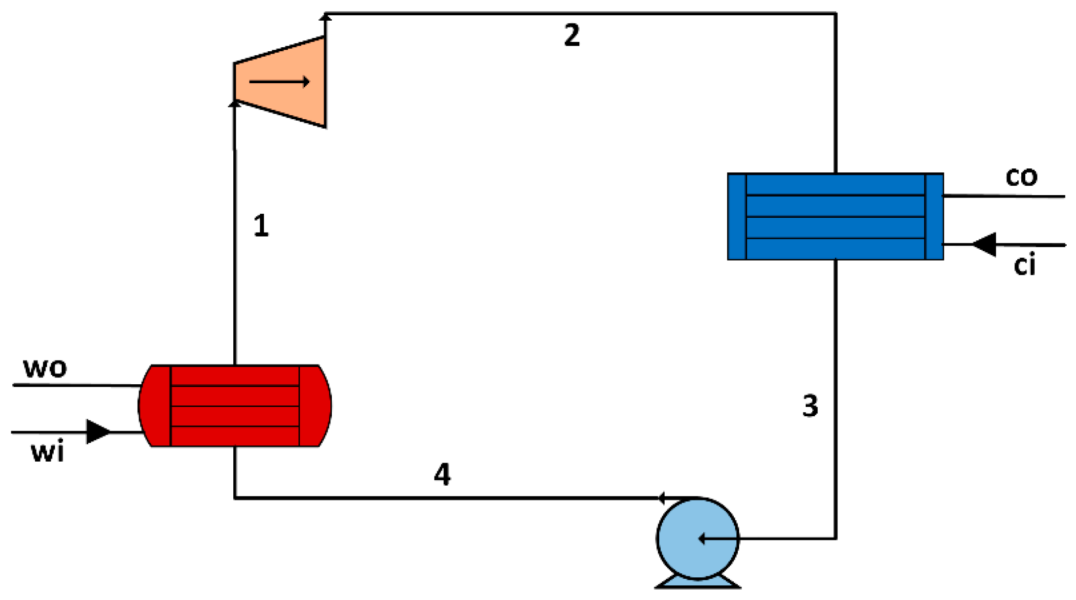
2.1. System Description

This study adopts the organic Rankine cycle as the cycle model for the ocean thermal energy conversion system. Figure 1 is a flow diagram of an ORC system. The cycle is composed of four key components: a working fluid pump, a turbo-expander, an evaporator, and a condenser.

R134a is a low-toxicity- and high-safety-class refrigerant. Sun [22] chose the type of working fluid considering the net output power of the ORC. It was found that the maximum net output power for R134a is near that of Ammonia, which has the same surface seawater flow rate, according to their findings. Therefore, this study selected R134a as the working fluid for the ORC. The working fluid pump is a canned pump that is completely leak-free, which pressurizes the low-pressure liquid working fluid to the evaporator. The evaporator is a flooded evaporator, which is a shell and tube heat exchanger with enhanced heat transfer tubes. The working fluid evaporates on the shell side of the evaporator and then enters the turboexpander to do work. The working fluid enters the condenser for condensation after leaving the turboexpander. The condenser is a shell and tube heat exchanger with enhanced heat transfer tubes. The working fluid condenses on the shell side of the condenser. The heat exchange tube is arranged in the upper half of the shell side in the condenser, and the cavity in the lower half can be used as a liquid storage tank.

This study assumes the temperatures of deep seawater and surface seawater, the length and diameter of the seawater pipe, the design efficiency of the turbine and pump, and the type of heat transfer pipe in the evaporator and condenser. The detailed information is given in

Table 1. The design conditions.

Parameters	Symbol	Value
Deep seawater temperature	$T_{ci}$	4 °C
Surface seawater temperature	$T_{wi}$	28 °C
Diameter of seawater pipe	$d_w$	0.35 m
Length of deep seawater pipe	$l_c$	3000 m
Length of surface seawater pipe	$l_w$	200 m
Design isentropic efficiency of turbine	${\eta }_t$	0.8
Design efficiency of generator	${\eta }_g$	0.9
Design efficiency of working fluid pump	${\eta }_p$	0.6
Design efficiency of seawater pump	${\eta }_w$	0.8
Type of heat transfer pipe in evaporator		Turbo BII
Number of heat transfer pipes in evaporator		478
Type of heat transfer pipe in condenser		Turbo CII
Number of heat transfer pipes in condenser		478
Working fluid		R134a

.

OTEC systems are suitable for the development and utilization of ocean thermal energy in sites where there is a steep topographic slope (15–20°) and a relatively smooth seafloor [23]. The steep topographic slope is 19.4° in Ref. [24]. This study assumes that the length of the deep seawater (at 1000 m depth) pipe is 3000 m, with a steep topographic slope of about 19.47°, in accordance with Refs. [23,24,25].

2.2. Mathematical Model

This study uses a flooded evaporator, and the state of the working fluid at the evaporator outlet is a saturated vapor state. The working fluid is condensed in the saturated liquid state at the condenser outlet. Under ideal cycle conditions, the relationship between the pressure at each point of the cycle and the evaporating pressure or condensing pressure is as follows:

$$P_{eva}=P_1=P_4$$

(1)

$$P_{con}=P_2=P_3$$

(2)

where $P_{eva}$ and $P_{con}$ are the evaporating pressure and condensing pressure, respectively, kPa; and $P_1$, $P_2$, $P_3,$ and $P_4$ are the absolute pressures of the working fluid at Points 1 to 4, shown in Figure 1, respectively, kPa.

2.2.1. Power Calculation

(1)

The turbine output electric power

The output electric power of the turbine generator is:

$$h_2=h_1-{\eta }_t\ast \left(h_1-h_{2s}\right)$$

(3)

$$W_t=m_r\left(h_1-h_2\right){\eta }_g$$

(4)

where $h_1$ and $h_2$ are the specific enthalpies at Point 1 and Point 2, respectively, kJ/kg;$h_{2s}$ is the isentropic enthalpy, kJ/kg; ${\eta }_t$ is the isentropic efficiency of the turbine; $m_r$ is the flow rate of the working fluid, kg/s; and ${\eta }_g$ is the efficiency of the generator.

(2)

The electric power consumption of the working fluid pump

The electric power consumption of the working fluid pump is:

$$W_p=\frac{m_r\ast \left(P_4-P_3\right)}{{\rho }_3{\eta }_p{\eta }_g}$$

(5)

$$h_4=h_3+W_p\ast {\eta }_g/m_r$$

(6)

where $W_p$ is the power consumption of the working fluid pump, kW; ${\rho }_3$ is the density of the working fluid at Point 3, kg/m³; ${\eta }_p$ is the efficiency of the pump; and $h_3$ and $h_4$ are the specific enthalpies at Point 3 and Point 4, respectively, kJ/kg.

(3)

The electric power consumption of the seawater pump

The electric power consumption of the surface seawater pump is:

$$W_{pw}=\frac{m_w\Delta P_w}{{\rho }_w{\eta }_w{\eta }_g}$$

(7)

$$\Delta P_w={\rho }_w{\lambda }_w\frac{l_w}{d_w}\frac{v_w{}^2}{2}$$

(8)

$$v_w=\frac{4m_w}{{\rho }_w\pi d_w^2}$$

(9)

where $m_w$ is the flow rate of the surface seawater, kg/s; $\Delta P_w$ is the pressure loss of the surface seawater flowing in the pipe caused by friction, kPa; ${\rho }_w$ is the density of seawater, kg/m³; ${\eta }_w$ is the efficiency of the seawater pump; ${\lambda }_w$ is the friction coefficient of the seawater pipe; $l_w$ is the length of the surface seawater pipe, m; $d_w$ is the diameter of the seawater pipe, m; and $v_w$ is the flow velocity of surface seawater, m/s.

The electric power consumption of the deep seawater pump is:

$$W_{pc}=\frac{m_c\Delta P_c}{{\rho }_w{\eta }_w{\eta }_g}$$

(10)

$$\Delta P_c={\rho }_w{\lambda }_w\frac{l_c}{d_w}\frac{v_c{}^2}{2}$$

(11)

$$v_c=\frac{4m_c}{{\rho }_c\pi d_w^2}$$

(12)

where $m_c$ is the flow rate of deep seawater, kg/s; $\Delta P_c$ is the pressure loss of the deep seawater flowing in the pipe caused by friction, kPa; $l_c$ is the length of the deep seawater pipe, m; and $v_c$ is the flow velocity of deep seawater, m/s.

The friction coefficient in commercial pipe is:

$$\frac{1}{\sqrt{\lambda }}=-2lg\left(\frac{\epsilon /d}{3.7}+\frac{2.51}{Re\sqrt{\lambda }}\right)$$

(13)

where $\epsilon$ is absolute roughness, 0.03 mm; $d$ is the diameter of the pipe, m; and $Re$ is the Reynolds number.

(4)

The net output power of the OTEC plant

The net output power of the OTEC plant is:

$$W_{net}=W_t-W_p-W_{pw}-W_{pc}$$

(14)

where $W_{net}$ is the net power of the OTEC, kW; $W_t$ is the output power of the turbine, kW; $W_p$ is the power consumption of the working fluid pump, kW; and $W_{pw}$ and $W_{pc}$ represent the pump’s consumption of surface seawater and deep seawater, kW.

2.2.2. Heat Transfer Area Calculation

The evaporator adopted in this study is a flooded evaporator, and the working fluid is in a saturated vapor state at the evaporator outlet. The condenser is a shell and tube heat exchanger, and the working fluid condenses to a saturated liquid state on the shell side of the condenser. The phase-change process is divided into two parts for both the evaporator and the condenser, as shown in Figure 2.

(1)

Heat transfer area of the evaporator

• The flow rate of the surface seawater

The flow rate of surface seawater is calculated based on the heat duty of the evaporating section.

$$Q_e=m_r\left(h_1-h_{eliq}\right)$$

(15)

$$m_w=\frac{Q_e}{c_{pwe}\left(T_{wi}-\mathsf{\Delta }{T}_w-T_e\right)}$$

(16)

where $Q_e$ is the heat duty of the phase change in the evaporator, kW; $h_{eliq}$ is the specific enthalpy of the saturated liquid at evaporating pressure, kJ/kg; $c_{pwe}$ is the constant pressure-specific heat capacity of surface seawater at the evaporating section, kJ/kg K;$T_{wi}$ is the surface seawater temperature at the evaporator inlet, °C; $T_e$ is the evaporating temperature, °C; and $\mathsf{\Delta }{T}_w$ is the pinch-point temperature difference for the evaporator, °C.

• The surface seawater temperature at the evaporator outlet

The outlet temperature of the surface seawater can be obtained according to the energy balance of the preheating section in the evaporator.

$$Q_{sc}=m_r\left(h_{eliq}-h_4\right)=m_w{c}_{pwsc}\left(T_e+\mathsf{\Delta }{T}_w-T_{wo}\right)$$

(17)

where $c_{pwsc}$ is the constant pressure-specific heat capacity of surface seawater at the preheating section, kJ/kg K; $T_{wo}$ is the surface seawater temperature at the evaporator outlet, °C; and $Q_{sc}$ is the heat duty of the preheating section in the evaporator, kW.

• The logarithmic mean temperature difference of the evaporator

The logarithmic mean temperature difference of the evaporating section is:

$${\mathsf{\Delta }\mathrm{T}}_{me}=\frac{\left(T_{wi}-T_e-\mathsf{\Delta }{T}_w\right)}{ln\frac{T_{wi}-T_e}{\mathsf{\Delta }{T}_w}}$$

(18)

The logarithmic mean temperature difference of the preheating section is:

$${\mathsf{\Delta }\mathrm{T}}_{msc}=\frac{\left(\mathsf{\Delta }{T}_w-T_{wo}+T_4\right)}{ln\frac{\mathsf{\Delta }{T}_w}{T_{wo}-T_4}}$$

(19)

where $T_4$ is the temperature of the working fluid at Point 4, °C.

• The heat transfer coefficient of the evaporator

The heat transfer coefficient of the working fluid on the outside surface of the single tube is:

$$h_{oe}=a{q}_e^b$$

(20)

where $q_e$ is the heat flux, kW/m². Coefficient $a$ = 2970.28 and $b$ = 0.549 when $q_e$ is less than 10 kW/m², otherwise $a$ = 16354 and $b$ = 0.035 [26].

The effect of the tube bundle on the heat transfer coefficient is related to the void fraction. Gorgy and Eckels [26] proposed an adaptation void fraction model based on the Feenstra, Weaver, and Judd model.

$$Ri=\frac{{\left({\rho }_l-{\rho }_g\right)}^{2}g\left(L_{tp}-d_o\right)}{G^2}$$

(21)

$$Ca=\frac{{\mu }_l}{\sigma }\frac{xG}{\epsilon {\rho }_g}$$

(22)

$$\epsilon ={\left(1+6.71\sqrt{Ri\ast Ca}\left(\frac{1-x}{x}\frac{{\rho }_g}{{\rho }_l}\right)\right)}^{-1}$$

(23)

$$\mathrm{G}=\frac{m_r}{\left(L_{tp}-d_o\right)L_e}$$

(24)

where $Ri$ is the Richardson number that represents a ratio between the buoyancy force and the inertia force [27]; $Ca$ is the capillary number that represents the ratio between the viscous force and the surface tension force; ${\rho }_l$ and ${\rho }_g$ are the density of the liquid phase and the density of the gas phase at the evaporation pressure, respectively; $L_{tp}$ is the tube pitch, 0.025 m; $d_o$ is the outside diameter of the heat transfer tube, 0.01905 m; $L_e$ is the length of the tube, m; $x$ is the quality; ${\mu }_l$ is the viscosity of the liquid, Pa·s; $\sigma$ is the surface tension, N/m; $\epsilon$ is the void fraction; and $G$ is the mass flux, kg/m²s;

The bundle heat transfer coefficient is:

$$F\ast h_{oe}={\left(\frac{1}{U_e}-\frac{1}{h_i}\frac{d_o}{d_i}-\frac{d_o}{2k_c}ln\frac{d_o}{d_i}\right)}^{-1}$$

(25)

where $F$ is the multiplication factor of the bundle on the heat transfer coefficient; $U_e$ is the average heat transfer coefficient, W/m² K; $k_c$ is the thermal conductivity of the heat transfer tube, 100.4 W/m K (HAL77-2); $d_i$ is the inside diameter of the heat transfer tube, 0.01605 m; and $h_i$ is the heat transfer coefficient of seawater in the heat transfer tubes, W/m² K, and is calculated using Formula (28).

The multiplication factor of the bundle on the heat transfer coefficient [26] is:

$$F_1=\frac{L_{tp}}{d_o}(1.52-2\ast {\left(0.96-\epsilon \right)}^2)$$

(26)

$$F_2=\frac{L_{tp}}{d_o}(0.81-2\ast {\left(0.75-\epsilon \right)}^2)$$

(27)

where $F$ is $F_1$ when the heat flux $q_e$ is less than 10 kW/m², otherwise $F$ is $F_2$.

The heat transfer coefficient of seawater flowing in the heat transfer tubes is:

$$h_i=C\frac{k_w}{d_i}\frac{f}{8}\frac{\left(Re-1000\right)Pr}{1+12.7\left(P{r}^{2/3}-1\right)\sqrt{f/8}}$$

(28)

$$f={\left(0.79\ln \left(Re\right)-1.64\right)}^{-2}$$

(29)

where $k_w$ is the thermal conductivity of seawater, W/(m K); $f$ is the friction factor of seawater flowing in the heat transfer tubes; $Pr$ is the Prandtl number; and $Re$ is the Reynolds number; $C$ is a constant, 1.928, which is used in Gorgy and Eckels [26].

• The heat transfer area calculation

The heat transfer area is:

$$A=\frac{Q}{U{\mathsf{\Delta }\mathrm{T}}_m}$$

(30)

$$U={\left(\frac{1}{h_o}+\frac{d_o}{h_i{d}_i}+\frac{d_o}{2\lambda }ln\frac{d_o}{d_i}\right)}^{-1}$$

(31)

where $U$ is the average heat transfer coefficient, W/m²K; ${\mathsf{\Delta }\mathrm{T}}_m$ is the logarithmic mean temperature difference, °C; $Q$ is the heat duty, kW; and $A$ is the heat transfer area, m².

(2)

Heat transfer area of the condenser

• The flow rate of the deep seawater

The flow rate of the deep seawater is:

$$m_c=\frac{Q_c}{c_{pc}\left(T_c-{\mathsf{\Delta }\mathrm{T}}_c-T_{ci}\right)}$$

(32)

$$Q_c=m_r\left(i_{cgas}-i_3\right)$$

(33)

where $Q_c$ is the heat duty of the phase change in the condenser, kW; $c_{pc}$ is the constant pressure-specific heat capacity of deep seawater at the condensing section, kJ/kg K; $T_{ci}$ is the deep seawater temperature at the condenser inlet, °C; $T_c$ is the condensing temperature, °C; ${\mathsf{\Delta }\mathrm{T}}_c$ is the pinch-point temperature of the condenser, °C; and $i_{cgas}$ is the specific enthalpy of the saturated vapor at condensing pressure, kJ/kg.

• The deep seawater temperature at the condenser outlet

The outlet temperature of the deep seawater can be obtained according to the energy balance of the precooling section in the condenser.

$$Q_{sh}=m_r\left(h_2-h_{cgas}\right)=m_c{c}_{pwsh}\left(T_{co}-T_c+\mathsf{\Delta }{T}_c\right)$$

(34)

where $c_{pwsh}$ is the constant pressure-specific heat capacity of deep seawater at the precooling section, kJ/kg K; $T_{co}$ is the deep seawater temperature at the condenser outlet, °C; and $Q_{sh}$ is the heat duty of the precooling section in the condenser, kW.

• The logarithmic mean temperature difference of the condenser

The logarithmic mean temperature difference of the condenser is:

$${\mathsf{\Delta }\mathrm{T}}_{mc0}=\frac{\left(T_c-T_{ci}-\mathsf{\Delta }{T}_c\right)}{ln\frac{T_c-T_{ci}}{\mathsf{\Delta }{T}_c}}$$

(35)

$${\mathsf{\Delta }\mathrm{T}}_{msh}=\frac{\left(T_2-T_{co}-\mathsf{\Delta }{T}_c\right)}{ln\frac{T_2-T_{co}}{\mathsf{\Delta }{T}_c}}$$

(36)

$${\mathsf{\Delta }\mathrm{T}}_{mc}=\frac{Q_c+Q_{sh}}{\frac{Q_c}{{\mathsf{\Delta }\mathrm{T}}_{mc0}}+\frac{Q_{sh}}{{\mathsf{\Delta }\mathrm{T}}_{msh}}}$$

(37)

where $T_2$ is the temperature of the working fluid at Point 2, °C.

• The heat transfer coefficient of the condenser

Kedzierski et al. [28] developed a model for predicting condensation on a Turbo-CII tube. The condensation heat flux of this model is:

$$q_c=\frac{0.683\left(1-c_b\right)}{p_f}{\left(\frac{\xi {\rho }_l{h}_{fg}{k}_l^3\mathsf{\Delta }{T}_s^3\sigma }{4{\mu }_l}\right)}^{1/4}$$

(38)

$$c_b=\frac{1}{\pi }co{s}^{-1}\left(1-\frac{4\sigma }{{\rho }_{l}g{d}_o{S}_r}\right)$$

(39)

$$\mathsf{\Delta }{T}_s=\frac{q_c}{h_{oc}}$$

(40)

$$h_{oc}={\left(\frac{1}{U_c}-\frac{1}{h_w}\frac{d_o}{d_i}-\frac{d_o}{2k_c}ln\frac{d_o}{d_i}\right)}^{-1}$$

(41)

where $p_f$ is fin pitch, 1/1575 m; $c_b$ is the fraction of the tube circumference flooded by condensate; $k_l$ is the thermal conductivity of the liquid working fluid, W/m K; $\mathsf{\Delta }{T}_s$ is the temperature difference between the wall temperature and the saturated working fluid, °C; $h_{fg}$ is the specific enthalpy difference of the working fluid between the condenser inlet and outlet, kJ/kg; $\xi$ is a dimensional constant and set to 1 m; $\sigma$ is the surface tension, N/m; ${\mu }_l$ is the dynamic viscosity, kg/m s; $S_r$ is the spacing between the fins at the fin root, 5.1 × 10⁻⁴ m; and $h_{oc}$ is the heat transfer coefficient at the outside of the condensate tube, W/m² K.

$h_{fg}$ is the latent heat of the working fluid in the model proposed in Ref. [28]. However, the working fluid at the turbine outlet has a small superheat degree since it is required to control the working fluid and not to liquefy in the turbine. Therefore, the $h_{fg}$ value in the model needs to be replaced by the specific enthalpy difference between the superheated vapor phase and the saturated liquid phase of the working fluid when predicting condensation on a Turbo-CII tube [29].

The condensation liquid film on the outside of tubes is the main source of resistance in the condensation process. It can be seen from Ref. [30] that the heat transfer coefficient on the tube rows near the condenser inlet can remain basically unchanged due to gas purging and the heat transfer coefficient higher than that on the tube rows far away from the condenser inlet. Therefore, the diffuser of the turbine is assumed to cancel in this study, and the high-speed gas at the turbine impeller outlet is used to purge the condenser to improve the condensation effect. It is assumed that this high-velocity gas purging removes the obstruction of the condensation process by the liquid film.

The heat transfer coefficient of the water side in the condenser can also be calculated using Equations (26) and (27), and the heat transfer area of the condenser can be calculated using Equation (28).

2.2.3. Method

In this study, we wrote a Matlab calculation program based on the above mathematical model; the calculation flowchart of the Matlab program is shown in Figure 3. The multi-objective optimization was performed by the gamultiobj solver (multi-objective optimization using Genetic Algorithm, which is a variant of NSGA-II [31]) in the optimization toolbox of Matlab. In the calculation process, the population of the genetic algorithm is constrained and screened by constraining the quality of the working fluid at the turbine outlet and the positive and negative of the net output power of the entire OTEC system.

(1)

the objective functions

The optimization objectives are set to maximize the net output power per unit heat exchange area and the exergy efficiency of the OTEC plant in the optimization design.

The net output power per unit heat exchange area is:

$$\gamma =\frac{W_{net}}{A_{eva}+A_{con}}$$

(42)

The exergy efficiency of OTEC plant is:

$${\eta }_{ex}=\frac{W_{net}}{E_{xwi}+E_{xci}}$$

(43)

$$E_{xwi}=m_w\left(\left(h_{wi}-h_{ref}\right)-T_{ref}\ast \left(s_{wi}-s_{ref}\right)\right)$$

(44)

$$E_{xci}=m_c\left(\left(h_{ci}-h_{ref}\right)-T_{ref}\ast \left(s_{ci}-s_{ref}\right)\right)$$

(45)

where the recommended values of temperature and pressure at the reference state are 293.15 K and 101.325 kPa, respectively; $h_{wi}$ and $h_{ci}$ are the specific enthalpies of the surface seawater and the deep seawater at the inlet of the evaporator and condenser, respectively, kJ/kg; $h_{ref}$ is the specific enthalpy of the seawater at the reference state, kJ/kg; $s_{wi}$ and $s_{ci}$ are the specific entropies of the surface seawater and the deep seawater at the inlets of the evaporator and the condenser, respectively, kJ/kg-K; and $s_{ref}$ is the specific entropy of the seawater at the reference state, kJ/kg-K;

(2)

The constraints on the decision variable range

In addition to the two constraints of turbine outlet quality and positive net output power, the ranges of the decision variables also need to be constrained. The decision variables include the working fluid flow rate, evaporating temperature, condensing temperature, and the pinch-point temperature difference between the evaporator and condenser in this study. The range constraints are as follows.

$$T_e+\Delta T_w\le 27.9<28=T_{wi}$$

(46)

$$-T_c+\Delta T_c\le -4.1<-4=-T_{ci}$$

(47)

$$5 \le m_r\le 13$$

(48)

$$17\le T_e\le 27$$

(49)

$$5\le T_c\le 15$$

(50)

$$0.5\le \Delta T_w, \Delta T_c\le 5$$

(51)

(3)

the evaluation indexes

The results of multi-objective optimization are a set of non-inferior solutions. In addition to the objective functions, there are many meaningful performance parameters of the OTEC system which can be used to evaluate these non-inferior solutions. These meaningful performance parameters include the thermal efficiencies of the OTEC (${\eta }_{OTEC}$) and ORC (${\eta }_{ORC}$), the back work ratio (BWR), the net output power ($W_{net}$), the net output power per unit of seawater flow ($WPSF$), the cold seawater flow ($m_c$), and the investment cost (Cost), etc.

$${\eta }_{OTEC}=\frac{W_{net}}{Q_e+Q_{sc}}$$

(52)

$${\eta }_{ORC}=\frac{W_t-W_p}{Q_e+Q_{sc}}$$

(53)

$$BWR=1-\frac{W_{net}}{W_t}$$

(54)

$$WPSF=\frac{W_{net}}{m_w+m_c}$$

(55)

$$Cost=\frac{CEPCI2017}{CEPCI2001}\ast C_{PI2001}$$

(56)

$$C_{PI2001}=C_{bm,e}+C_{bm,c}+C_{bm,t}+C_{bm,p}+C_{bm,pw}+C_{bm,pc}$$

(57)

$$C_{bm}=C_p\ast F_{bm}$$

(58)

$$\lg C_p=K_1+K_2\lg Z+K_3{\left(\lg Z\right)}^2$$

(59)

$$F_{bm}=B_1+B_2{F}_m{F}_p$$

(60)

$$\lg F_p=C_1+C_2\lg P+C_3{\left(\lg P\right)}^2$$

(61)

where $Z$ is the heat transfer area of the evaporator and condenser, m², and the shaft power of the turbine and pump, kW; and $P$ is the operating pressure, barg. The $CEPCI2001$ and all coefficients, including $K_1$, $K_2$, $K_3$, $C_1$, $C_2$, $C_3$, $F_{bm}$ (or $B_1$, $B_2$, $F_m$) of evaporator(fixed tube sheet), condenser(fixed tube sheet), pump(carbon steel, centrifugal) and steam turbine, refer to Ref. [32]. The $CEPCI2017$ is 628.2 [33].

3. Results

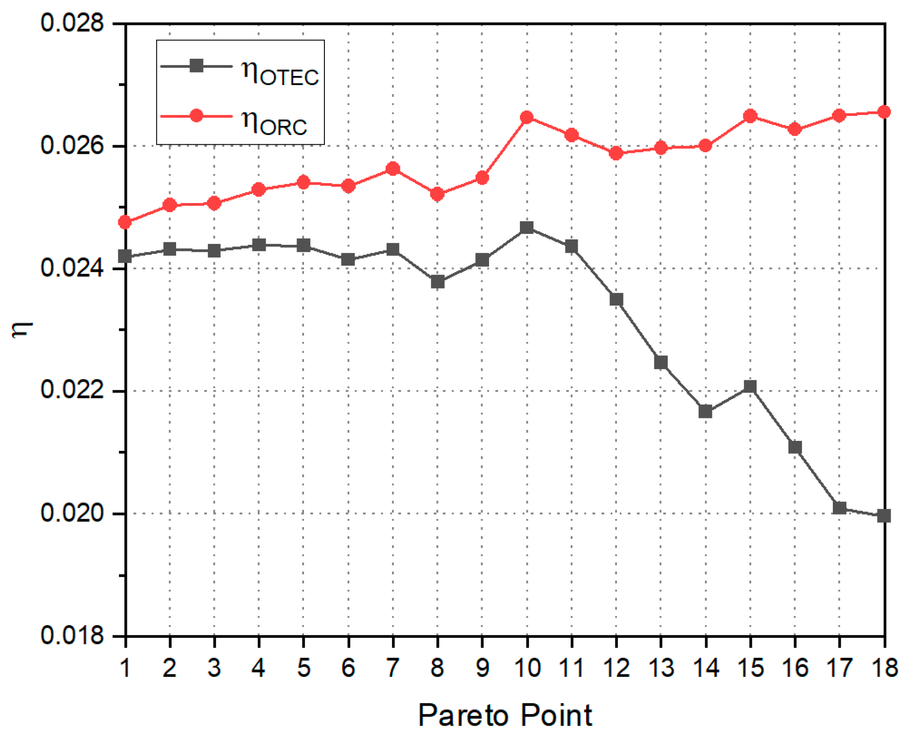
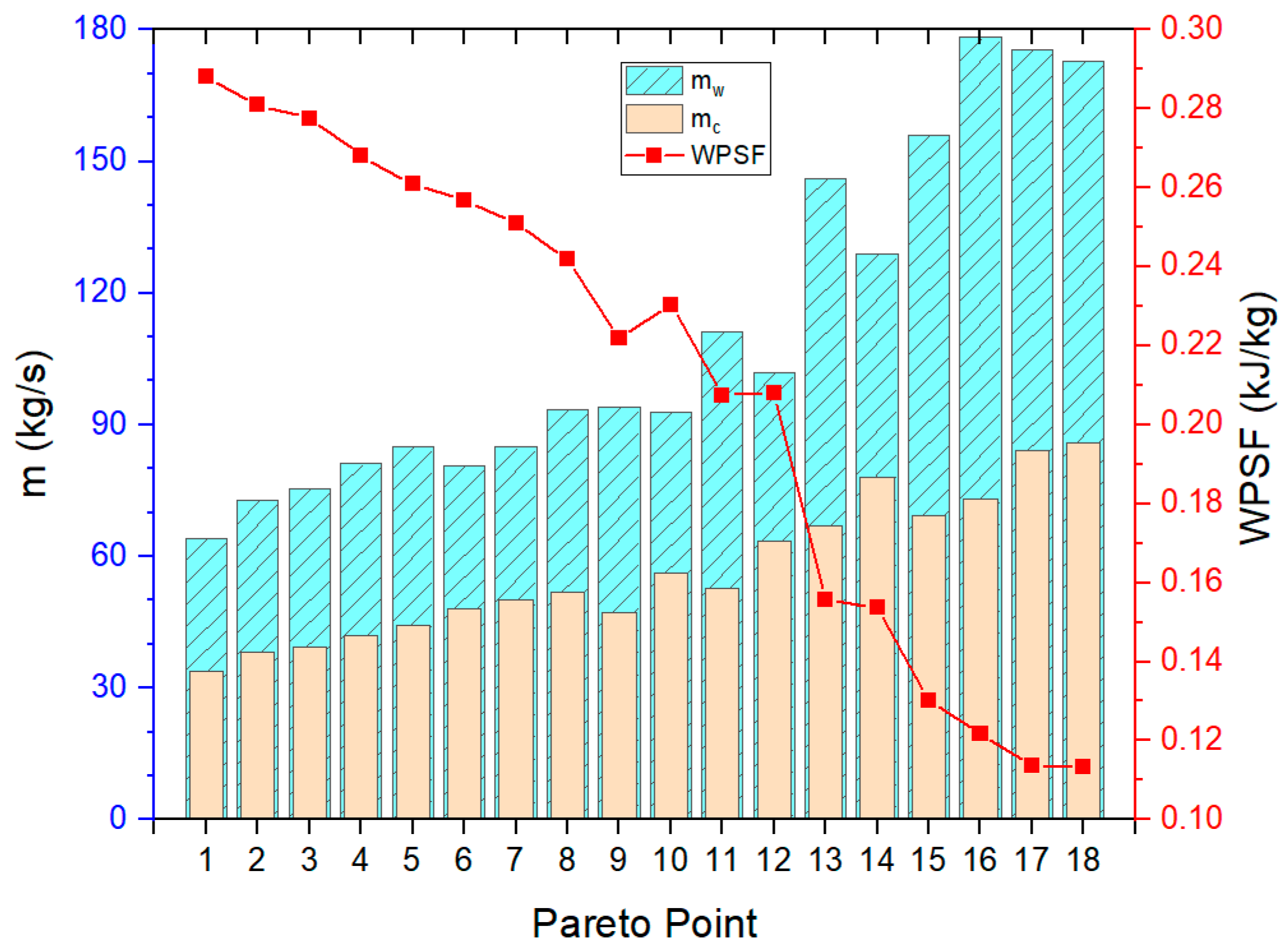
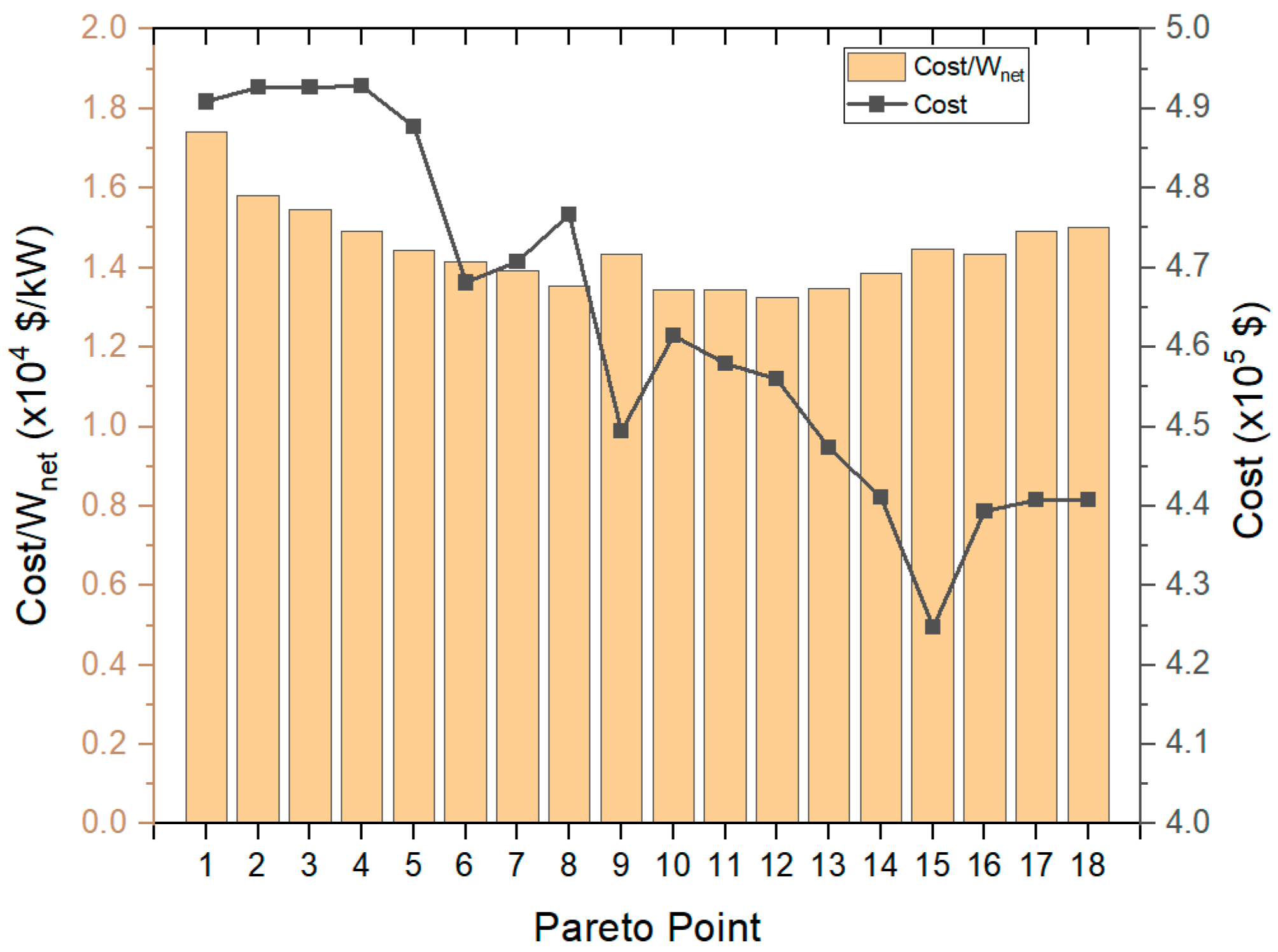
3.1. The Optimization Design Results

The multi-objective optimization results are shown in Figure 4. The Pareto front consists of 18 results. The point that is closest to Point A (the ideal point) is Point 11 among the 18 Pareto frontier points, and the next closest is Point 10.

Figure 5, Figure 6, Figure 7 and Figure 8 show the results of the evaluation indexes for the 18 Pareto points. The evaluation indexes of Point 10 are better than those for Point 11, except for economic cost. In the case that the economic cost deviation between Points 10 and 11 was not large, Point 10 was selected as the final solution in this study. The detailed results for the 18 Pareto points are listed in Appendix A. The state parameters at each point of the ORC under the final solution of Point 10 are shown in

Table 2. The optimal state parameters of the ORC under the solution of Point 10.

Point	Pressure (kPa)	Temperature (°C)	Enthalpy (kJ/kg)	Entropy (kJ/kg K)	Phase
1	631.09	23.24	411.43	1.7169	Saturated vapor
2	435.78	11.73	405.37	1.7222	Superheated, 0.23 °C
3	435.78	11.50	215.64	1.0557	Saturated liquid
4	631.09	11.67	215.91	1.0561	Subcooled, 11.57 °C

.

3.2. The Effects of Decision Parameters on the Performance of the OTEC

In this study, we kept the flow rate of the working fluid constant (that is, $m_r$ = 7.117 kg/s) and explored the influence of the other four decision variables on the performance of the OTEC system. In studying the effects of the evaporating temperature and condensing temperature, the pinch-point temperature difference was kept unchanged (that is, $\mathsf{\Delta }{T}_w$ = 1.48 °C and $\mathsf{\Delta }{T}_c$ = 1.78 °C). Conversely, the evaporating temperature and condensing temperature were kept unchanged (that is, $T_e$ = 23.24 °C, $T_c$ = 11.5 °C).

• The effects of evaporating temperature and condensing temperature

Figure 9a–d all show the same law. The exergy efficiency, the net output power per unit area, the net thermal efficiency, and the net output power increase first and then decrease with increase in evaporating temperature or condensing temperature.

Figure 9e illustrates how the flow rate of deep seawater increases with the decrease in condensing temperature. The seawater flow rate is determined by the latent heat of the working fluid according to Equation (32). The latent heat of the phase transition is related to the phase-change temperature. Under the condition that the seawater temperature at the condenser inlet and the pinch-point temperature difference are fixed, the deep seawater flow rate is only related to the phase-transition temperature. The variation in surface seawater flow rate with evaporating temperature in Figure 9f is consistent with this. The seawater flow rate increases clearly, mainly because the changes in seawater temperature at the inlet and outlet of the heat exchanger are too small at this point.

Figure 9g shows the effects of evaporating temperature and condensing temperature on the net output power per unit seawater flow rate (WPSF). The WPSF value in the A region is larger because the seawater flow rate is lower. The lower WPSF values in the C and E regions are mainly due to the higher seawater flow rate. Although the net output power in the B region is higher, the high seawater flow rate leads to a smaller WPSF value. The reason for the smaller WPSF value in the D region is opposite to that for the value in the B region. The seawater flow rate in the D region is small, but the net output power is also small, resulting in a small WPSF value.

It can be seen from Figure 9h that the back work ratio (BWR) is seriously affected by the condensing temperature. The condensing temperature is related to the deep seawater flow rate, which is related to the power consumption of the deep seawater pump. It can be concluded that it helps to decrease the BWR value by increasing the condensing temperature. It is worth noting that the net output power is not necessarily high when the BWR is high (comparing Figure 9h and Figure 9d).

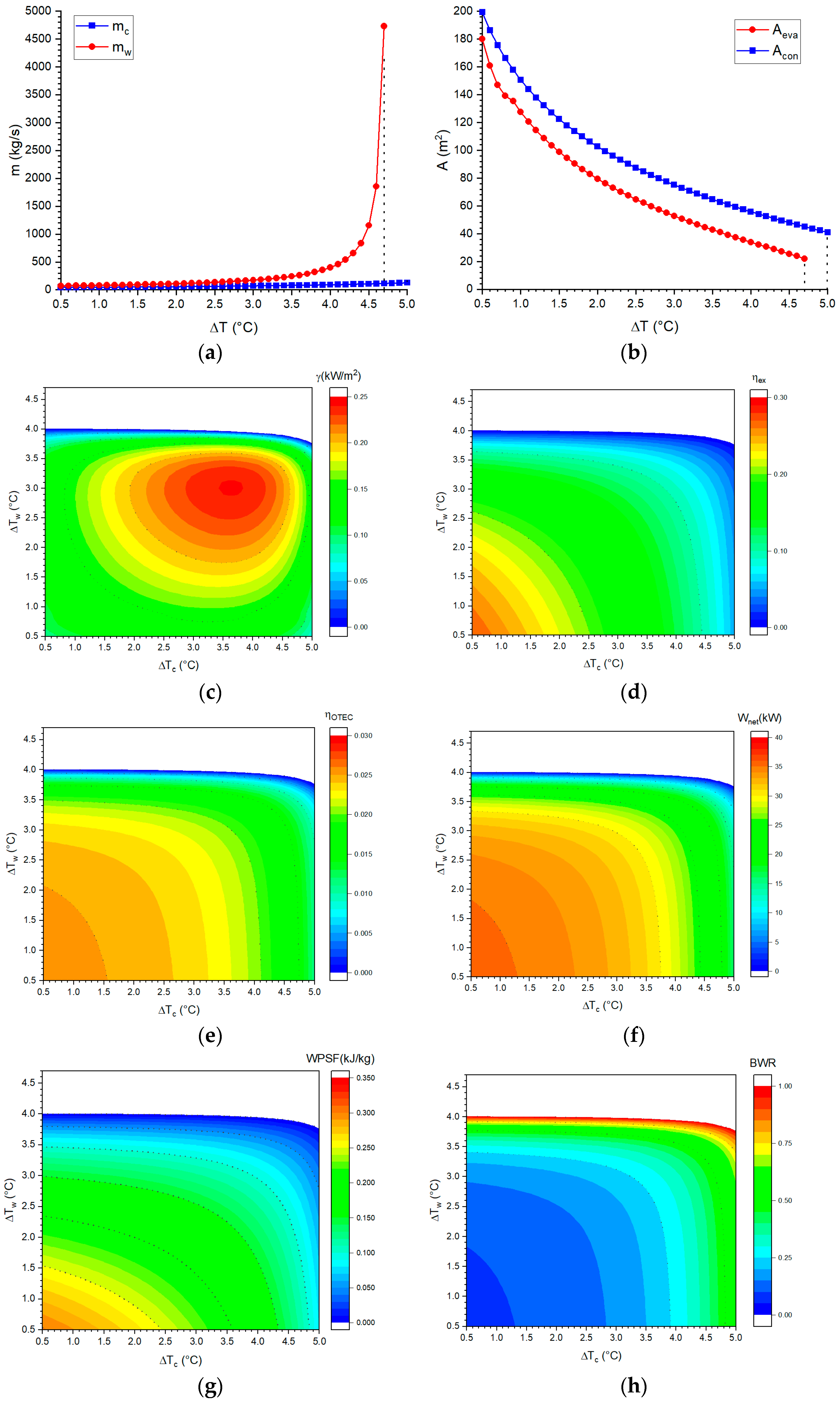
• The effect of the pinch-point temperature difference

When the evaporating temperature, condensing temperature, and flow rate of the working fluid are fixed, the gross output power of the turbine ($W_t$), the power consumption of the working fluid pump ($W_p$), and the heat exchange of the evaporator and condenser ($Q_e+Q_{sc}$ and $Q_c+Q_{sh}$) all remain unchanged, no matter how the pinch-point temperature difference changes. The parameters directly related to the pinch-point temperature difference are mainly the flow rate of the seawater, the area of the heat exchanger, and the seawater pump power consumption.

From Figure 10a,b, it can be seen that the larger the pinch-point temperature difference is, the smaller the heat exchanger area is but the higher the seawater consumption is. Seawater pump power is proportional to seawater flow rate.

From Figure 10c–h, it can be seen that the effects of $\Delta T_w$ and $\Delta T_c$ on the net output power per unit area (γ) are different from those of the other terms. This is because only the net output power per unit area is related to both seawater flow rate and heat transfer area. The other terms are only related to seawater flow rate. This results in all of the performance parameters except the net output power per unit area decreasing as the pinch-point temperature difference increases.

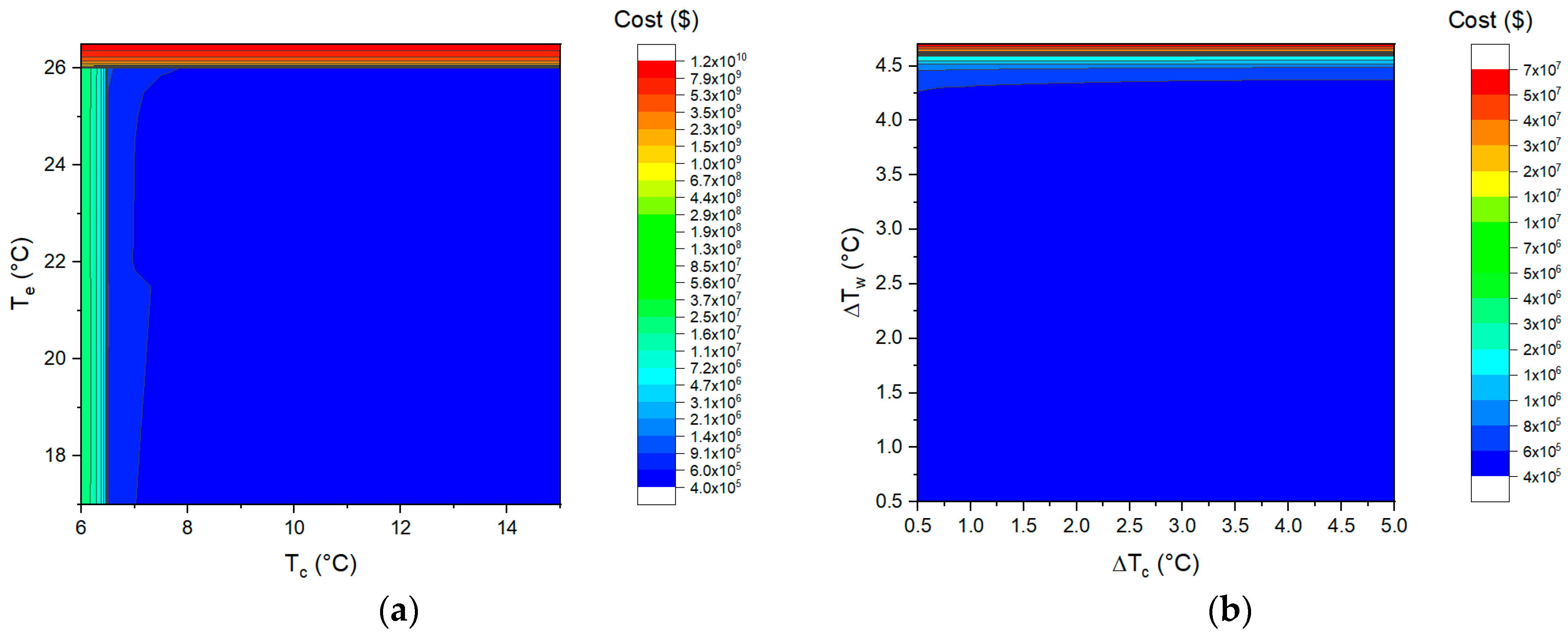
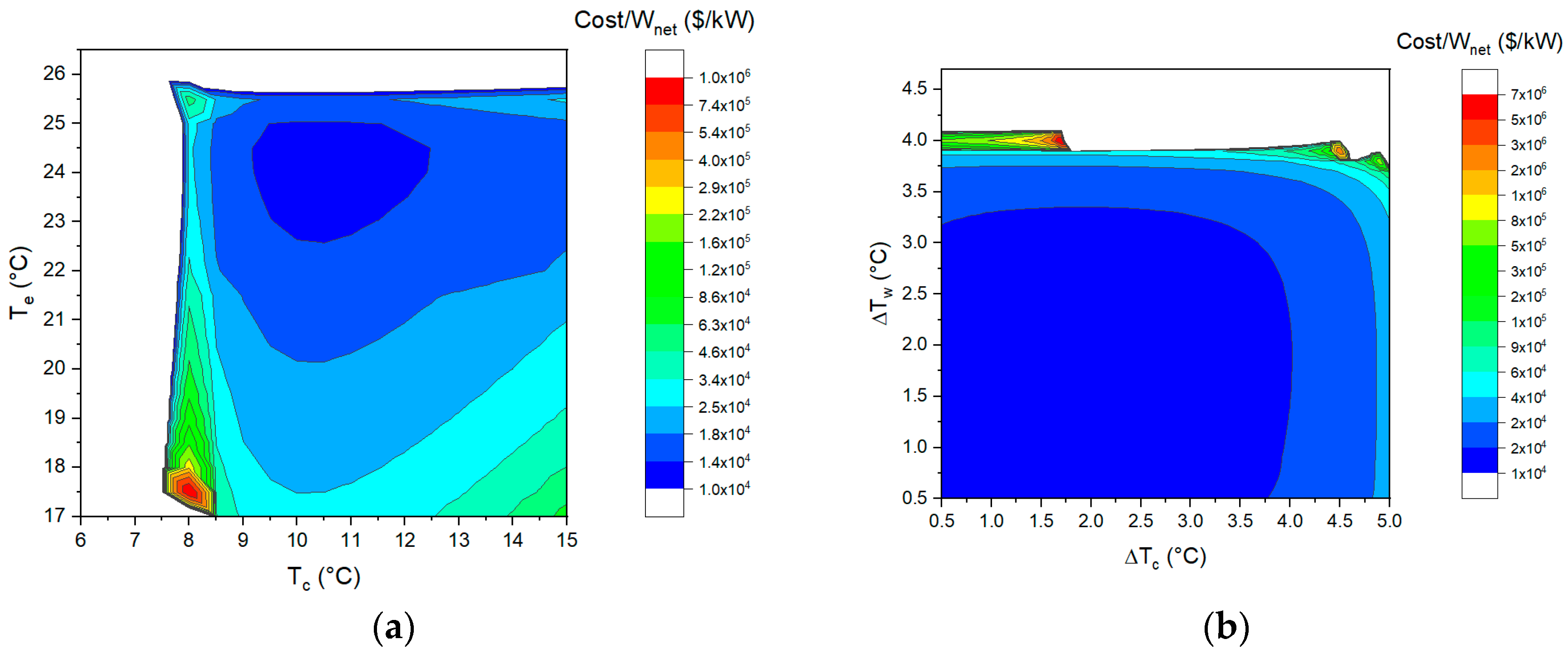
• The effect of the four decision parameters on the investment cost

As can be seen from Figure 11a, the smaller the difference between the evaporating temperature and the surface seawater temperature, the greater the equipment investment cost. The same holds for the condensing temperature and deep seawater temperature. Therefore, to reduce equipment costs, it should be optimized away from the seawater temperature. In addition, when optimizing the pinch-point temperature difference, the focus should be on the pinch-point temperature difference of the evaporator.

Comparing Figure 12a and Figure 9a, it can be seen that the effects of the evaporating temperature and condensing temperature on the net output power per unit heat exchange area are roughly similar to the effects of the investment cost per unit net output power. Figure 12b shows that the investment cost per unit net output power decreases with decreasing pinch-point temperature difference. The trend in Figure 12b is roughly similar to that in Figure 10f (the effect of the pinch-point temperature difference on the net output power) and not similar to that in Figure 10a (the net output power per unit heat exchange area), mainly because the investment cost is not very sensitive to the pinch-point temperature difference over a large range (as shown in Figure 11b).

4. Conclusions

The optimization goals of this study were to maximize the net output power per unit area and the exergy efficiency. This study obtained 18 Pareto frontier points through multi-objective optimization using a genetic algorithm. The following conclusions are drawn:

(1)

The exergy efficiency, the net output power per unit area, the net thermal efficiency, and the net output power increase first and then decrease with the increase in evaporating temperature or condensing temperature.

(2)

The back work ratio (BWR) is seriously affected by the condensing temperature. Increasing the condensing temperature can decrease the BWR value; however, the net output power is not necessarily large when the BWR is small.

(3)

The parameters directly related to the pinch-point temperature difference are, mainly, the flow rate of the seawater, the area of the heat exchanger, and the seawater pump power consumption. A small pinch-point temperature difference is beneficial for the performance parameters (the exergy efficiency, the thermal efficiency of the OTEC, the net output power, the net output power per unit seawater flow rate, and the back work ratio).

(4)

The investment cost is not very sensitive to the pinch-point temperature difference and evaporating temperature and condensing temperature over wide ranges. The effects of evaporating temperature and condensing temperature on the investment cost per unit net output power are roughly similar to those on the net output power per unit heat exchange area. However, the change in the investment cost per unit net output power with the pinch-point temperature difference is mainly determined by the change trend of the net output power.

References

- Zhang, J.; Tang, Z.; Qian, F. A review of recent advances and key technologies in ocean thermal energy conversion. J. Hohai Univ. 2019, 47, 55–64. [Google Scholar]
- Wang, C.; Lu, W. Analysis Method and Reserve Assessment of Ocean Energy Resources; Ocean Press: Beijing, China, 2009; p. 171. [Google Scholar]
- Vera, D.; Baccioli, A.; Jurado, F.; Desideri, U. Modeling and optimization of an ocean thermal energy conversion system for remote islands electrification. Renew. Energy 2020, 162, 1399–1414. [Google Scholar] [CrossRef]
- Shen, W. Analysis of Thermodynamic Cycle in Ocean Thermal Energy Conversion (OTEC) System; China University of Petroleum (East China): Qingdao, China, 2012. [Google Scholar]
- Kalina, A.I. Generation of Energy by Means of a Working Fluid, and Regeneration of a Working Fluid. U.S. Patent US04346561A, 31 August 1982. [Google Scholar]
- Uehara, H.; Ikegami, Y.; Fukugawa, H.; Uto, M. Performance Analysis of OTEC System Using Kalina Cycle. Thermodynamic Characteristics of Cycle. Trans. Jpn. Soc. Mech. Eng. Part B 1994, 60, 3519–3525. [Google Scholar] [CrossRef]
- Uehara, H.; Ikegami, Y.; Nishida, T. Performance Analysis of OTEC System Using a Cycle with Absorption and Extraction Processes. Trans. Jpn. Soc. Mech. Eng. Ser. B 1998, 64, 2750–2755. [Google Scholar] [CrossRef]
- Satoru, G.; Yoshiki, M.; Takenao, S.; Takeshi, Y.; Yasuyuki, I.; Masatoshi, N. Construction of simulation model for OTEC plant using Uehara cycle. Electr. Eng. Jpn. 2011, 176, 1–13. [Google Scholar]
- Liu, W.M.; Chen, F.Y.; Wang, Y.Q.; Jiang, W.J. Progress of Closed-Cycle OTEC and Study of a New Cycle of OTEC. Adv. Mater. Res. 2012, 354–355, 275–278. [Google Scholar] [CrossRef]
- White, H.J. Mini-OTEC. Int. J. Ambient. Energy 1980, 1, 75–88. [Google Scholar] [CrossRef]
- Negara, R.B.; Koto, J. Potential of 100 kW of Ocean Thermal Energy Conversion in Karangkelong, Sulawesi Utara, Indonesia. Int. J. Environ. Res. Clean Energy 2017, 5, 1–10. [Google Scholar]
- Yang, M.H.; Yeh, R.H. Analysis of optimization in an OTEC plant using organic Rankine cycle. Renew. Energy 2014, 68, 25–34. [Google Scholar] [CrossRef]
- Uehara, H.; Ikegami, Y. Optimization of a Closed-Cycle OTEC System. Trans Asme J. Sol. Energy Eng. 1990, 112, 247–256. [Google Scholar] [CrossRef]
- Bernardoni, C.; Binotti, M.; Giostri, A. Techno-economic analysis of closed OTEC cycles for power generation. Renew. Energy 2018, 132, 1018–1033. [Google Scholar] [CrossRef]
- Najafi, A.; Rezaee, S.; Torabi, F. Multi-objective optimization of ocean thermal energy conversion power plant via genetic algorithm. In Proceedings of the 2011 IEEE Electrical Power and Energy Conference, Winnipeg, MB, Canada, 3–5 October 2011. [Google Scholar]
- Zhang, S.R.; Sun, Y.S.; Wang, M.T.; Jang, L.X.; Liu, Q.Y. Multi-objective function optimization study on ocean thermal energy organic rankine cycle systems. Renew. Energy Resour. 2017, 35, 621–626. [Google Scholar]
- Wang, M.; Zhao, Y.; Zhang, H.; Wang, B. Multi-objective Optimization of OTEC Rankine Cycle based on PSO Algorithm. Chin. J. Sol. Energy 2019, 40, 2716–2724. [Google Scholar]
- Hettiarachchi, H.; Golubovic, M.; Worek, W.M. Optimum design criteria for an Organic Rankine cycle using low-temperature geothermal heat sources. Energy 2007, 32, 1698–1706. [Google Scholar] [CrossRef]
- Wang, J.; Yan, Z.; Man, W. Multi-objective optimization of an organic Rankine cycle (ORC) for low grade waste heat recovery using evolutionary algorithm. Energy Convers. Manag. 2013, 71, 146–158. [Google Scholar] [CrossRef]
- Ahmadi, P.; Dincer, I.; Rosen, M.A. Thermoeconomic multi-objective optimization of a novel biomass-based integrated energy system. Energy 2014, 68, 958–970. [Google Scholar] [CrossRef]
- Jiang, L.; Zhu, Y.D.; Jin, V.; Yu, L.J. Comprehensive Evaluation Method of ORC System Performance Based on the Multi-Objective Optimization. Adv. Mater. Res. 2014, 997, 721–727. [Google Scholar] [CrossRef]
- Sun, F.; Ikegami, Y.; Jia, B.; Arima, H. Optimization design and exergy analysis of organic rankine cycle in ocean thermal energy conversion. Appl. Ocean. Res. 2012, 35, 38–46. [Google Scholar] [CrossRef]
- Song, Z.; Ye, L.; Yang, B.; Yisen, Z.; Qingwei, Z.; Xiaoyong, W.; Min, D.; Jie, M.; Hao, X. An assessment of ocean thermal energy conversion resources in the South China Sea. In Proceedings of the OCEANS 2016–Shanghai, Shanghai, China, 10–13 April 2016. [Google Scholar]
- Jitsuhara, S.; Ikegami, Y.; Uehara, H. Optimization of Design Conditions for OTEC. In the Case of Annual Operation Performance. Trans. Jpn. Soc. Mech. Eng. Part B 1994, 60, 641–648. [Google Scholar] [CrossRef][Green Version]
- Giostri, A.; Romei, A.; Binotti, M. Off-design performance of closed OTEC cycles for power generation. Renew. Energy 2021, 170, 1353–1366. [Google Scholar] [CrossRef]
- Gorgy, E.; Eckels, S. Convective boiling of R-134a on enhanced-tube bundles. Int. J. Refrig. 2016, 68, 145–160. [Google Scholar] [CrossRef]
- Thome, J.R. Engineering Data Book III; Wolverine Tube Inc.: Decatur, AL, USA, 2004; Volume 5, pp. 17–25. [Google Scholar]
- Kedzierski, M.A.; Carr, M.A.; Brown, J.S. Measurement and Prediction of Vapor-Space Condensation of Refrigerants on Trapezoidal-Finned and Turbo-C Geometries. J. Enhanc. Heat Transf. 2013, 20, 59–71. [Google Scholar] [CrossRef]
- Tong, J.; Zhao, Z. Thermal Engineering Foundation; Higher Education Press: Beijing, China, 2009; p. 246. [Google Scholar]
- Huber, J.B. Shell-Side Condensation of HFC-134a and HCFC-123 on Enhanced-Tube Bundles; Iowa State University: Ames, IA, USA, 1994. [Google Scholar]
- Available online: https://ww2.mathworks.cn/help/gads/gamultiobj-algorithm.html (accessed on 25 August 2022).
- Turton, R. Analysis, Synthesis and Design of Chemical Processes; (Appendix A); Prentice Hall International: Hoboken, NJ, USA, 2008. [Google Scholar]
- Borugadda, V.B.; Kamath, G.; Dalai, A.K. Techno-economic and life-cycle assessment of integrated Fischer-Tropsch process in ethanol industry for bio-diesel and bio-gasoline production. Energy 2020, 195, 116985.1–116985.6. [Google Scholar] [CrossRef]