

Machine Learning Methods to Forecast the Concentration of PM10 in Lublin, Poland


Abstract
:1. Introduction
2. Materials and Methods
2.1. The Dataset
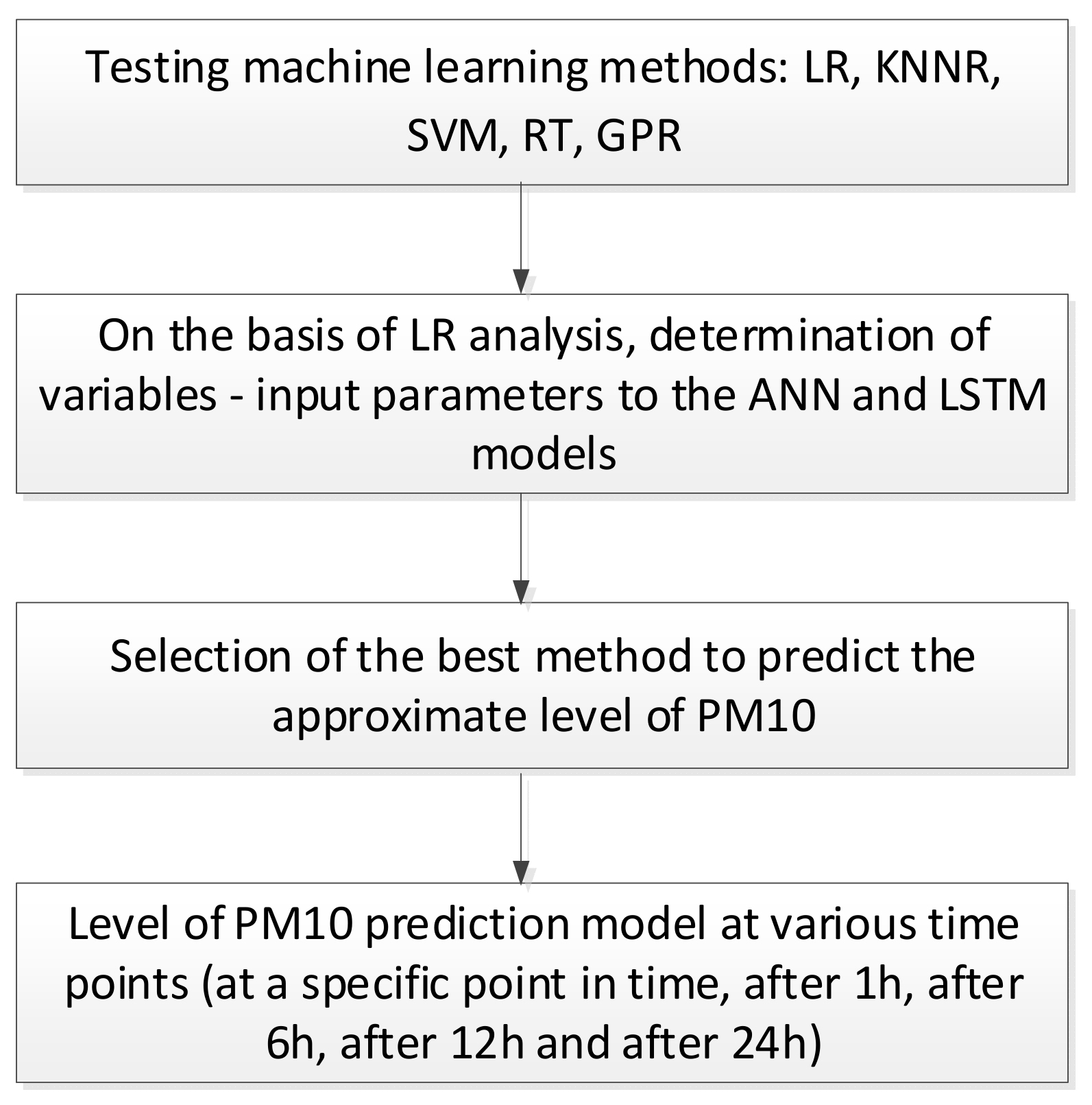
2.2. Methods
3. Results
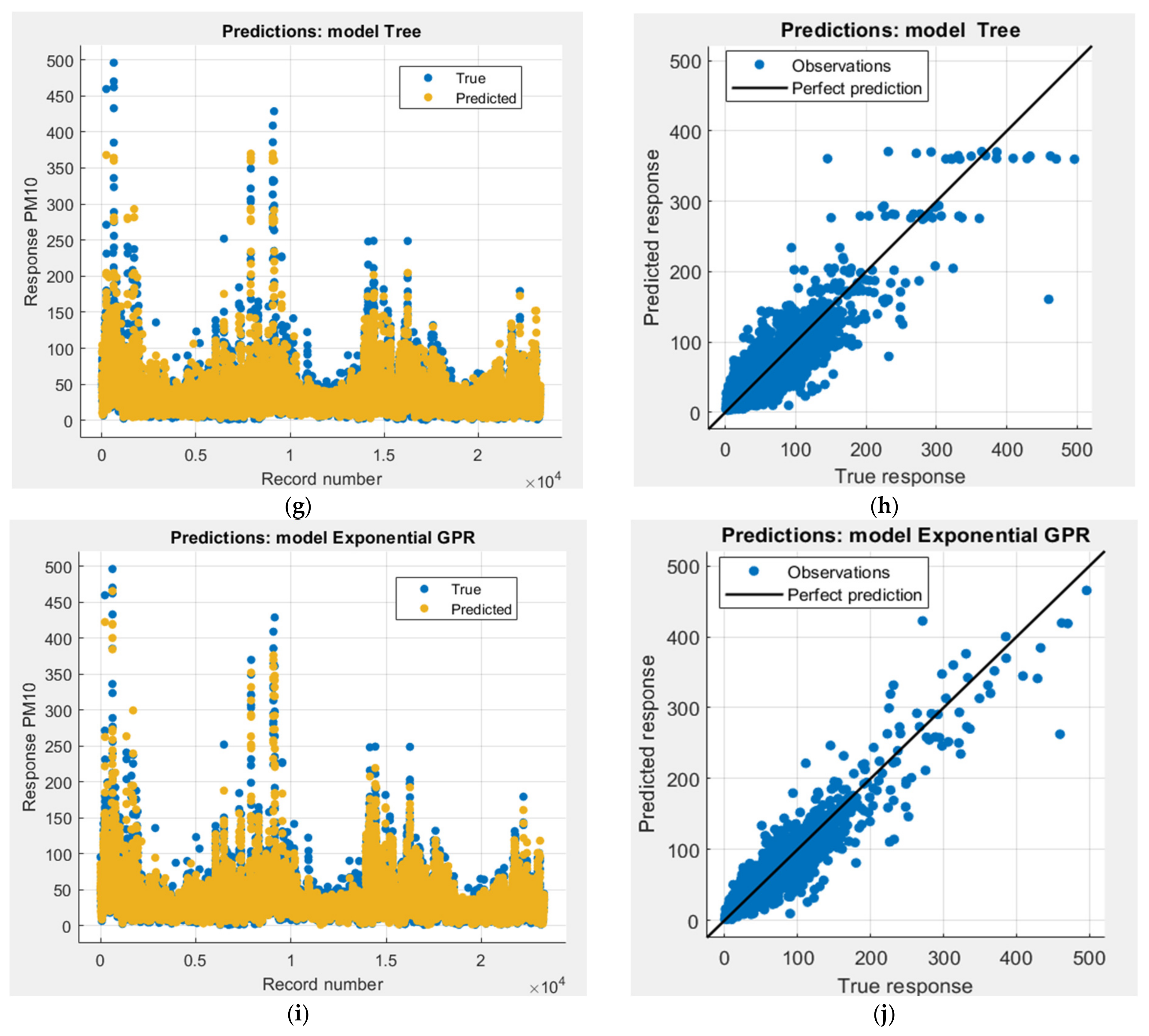
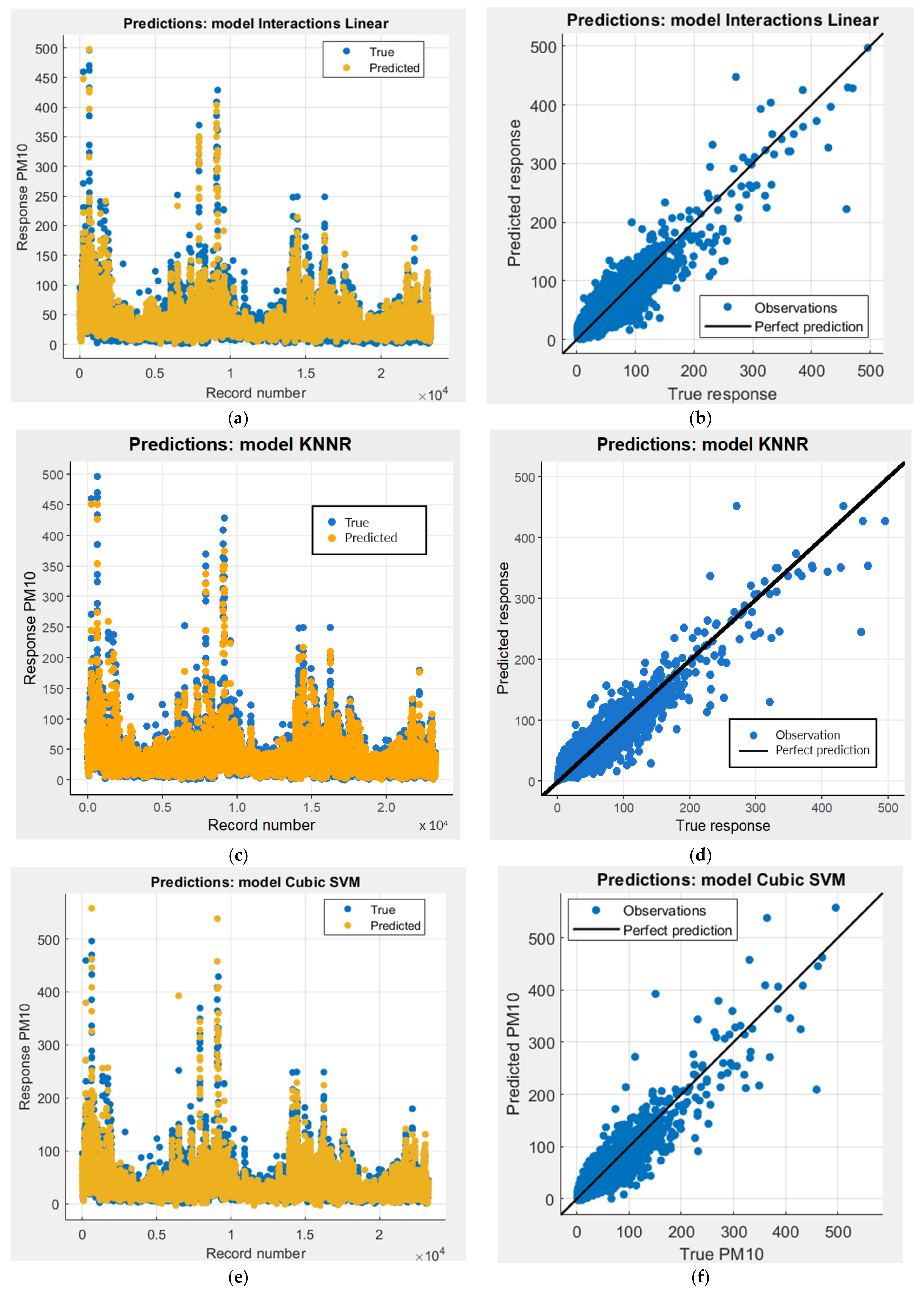
3.1. Models Obtained Using Machine Learning Methods
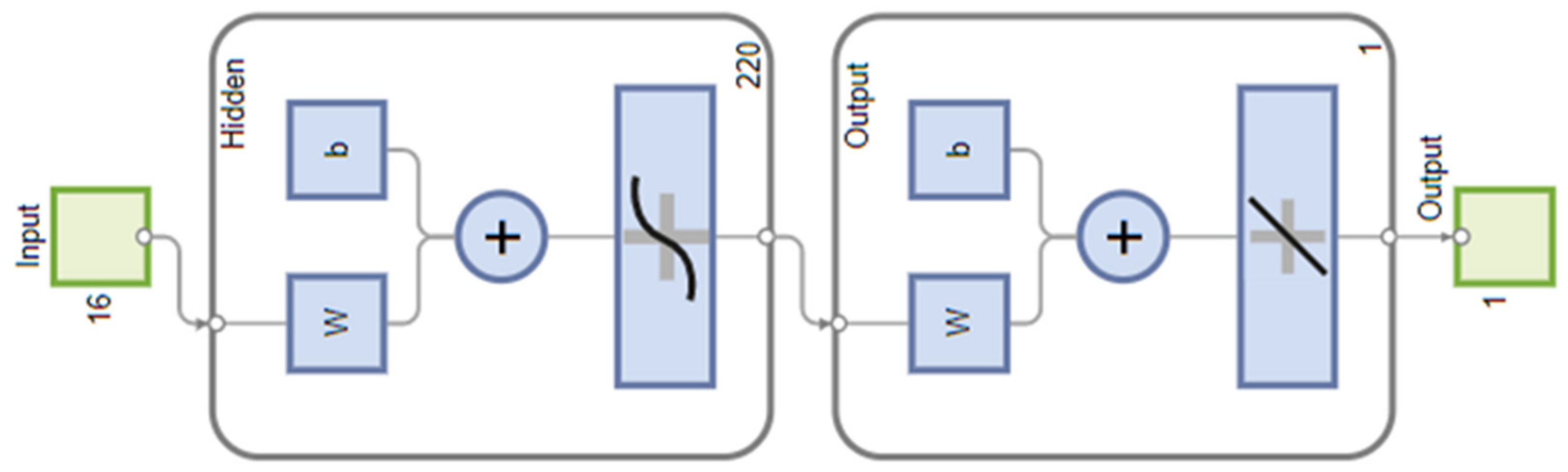
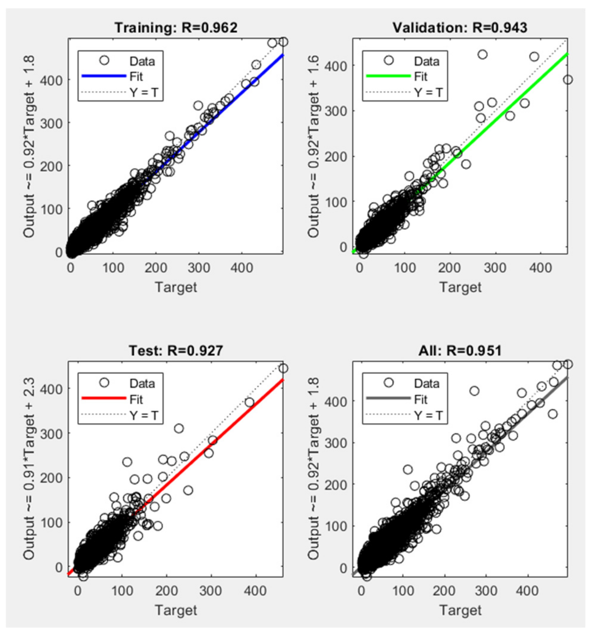
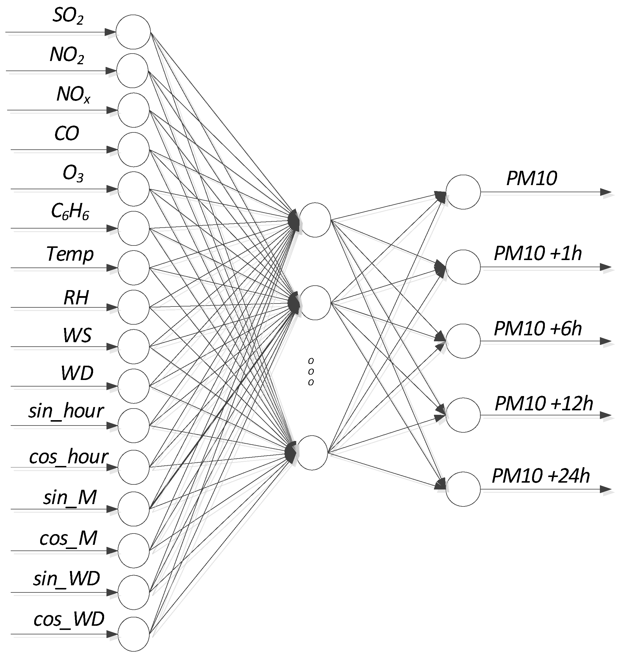
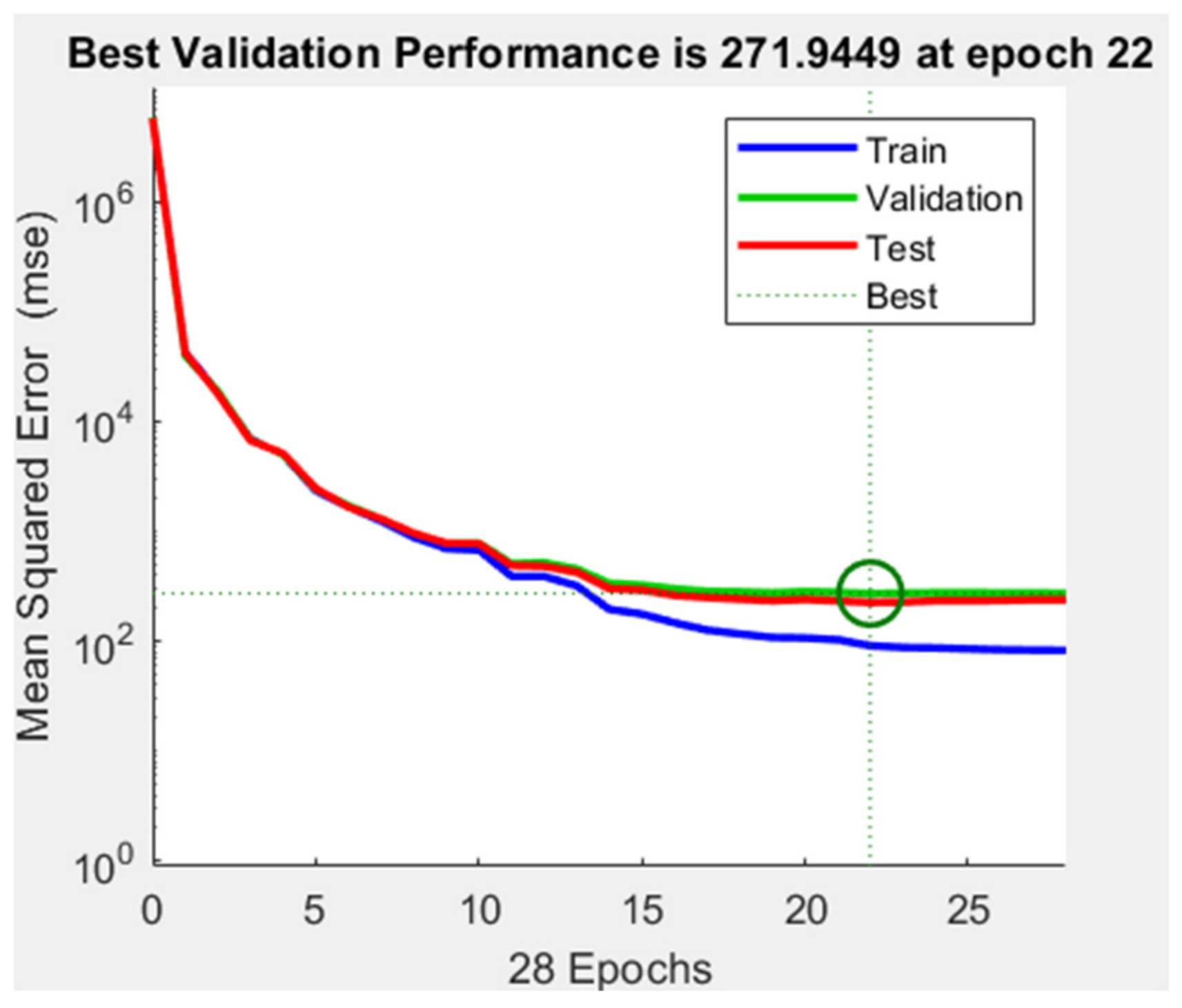
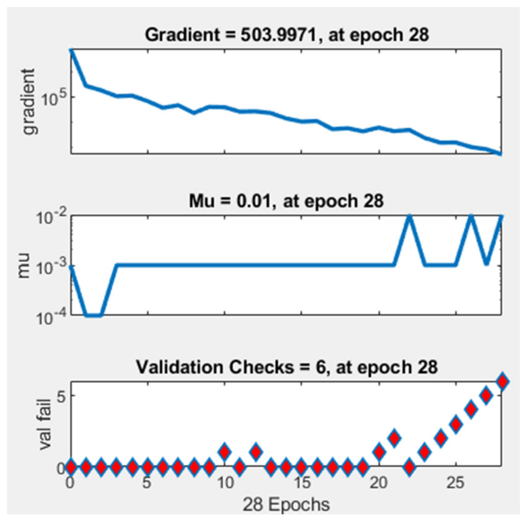
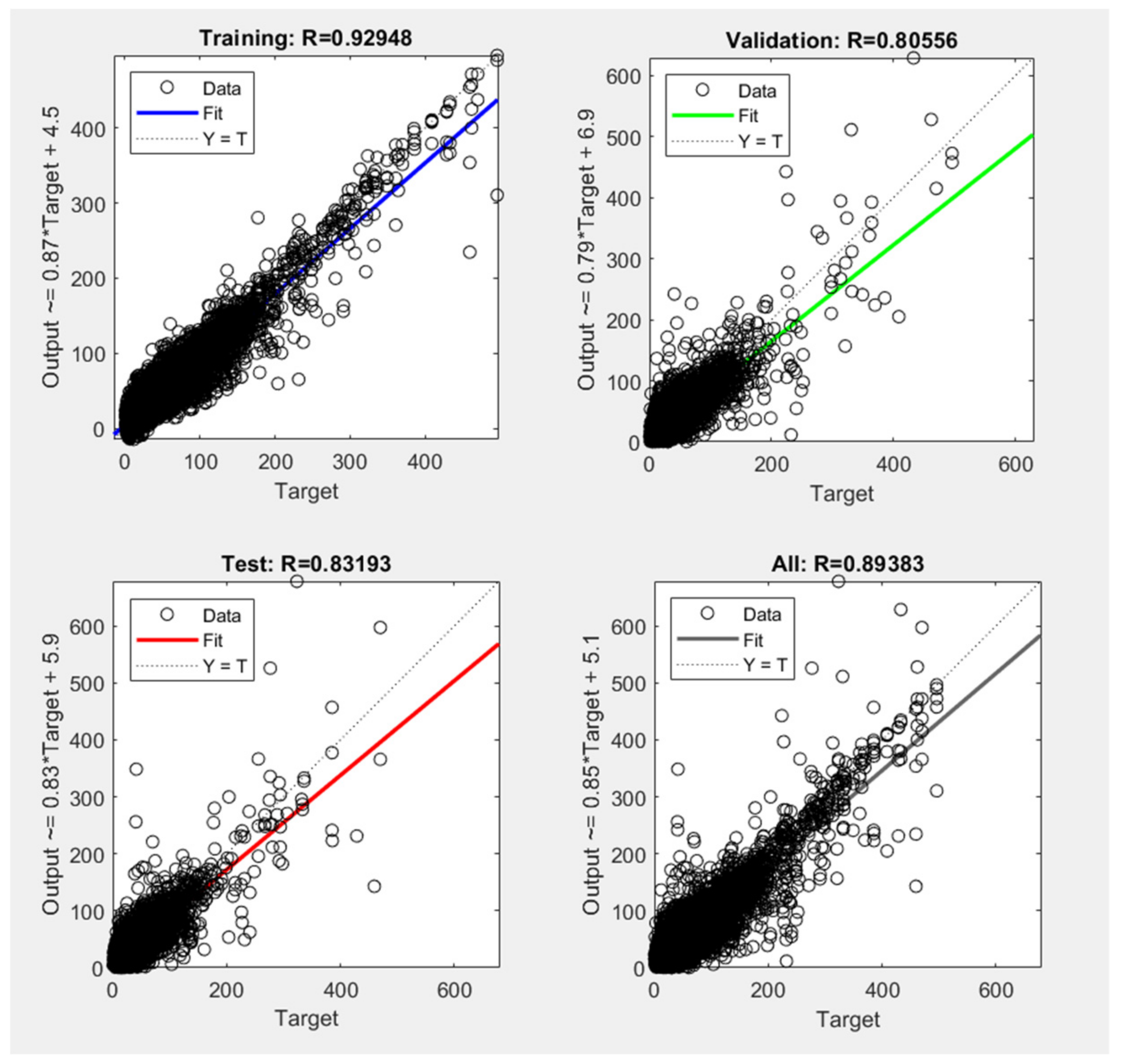
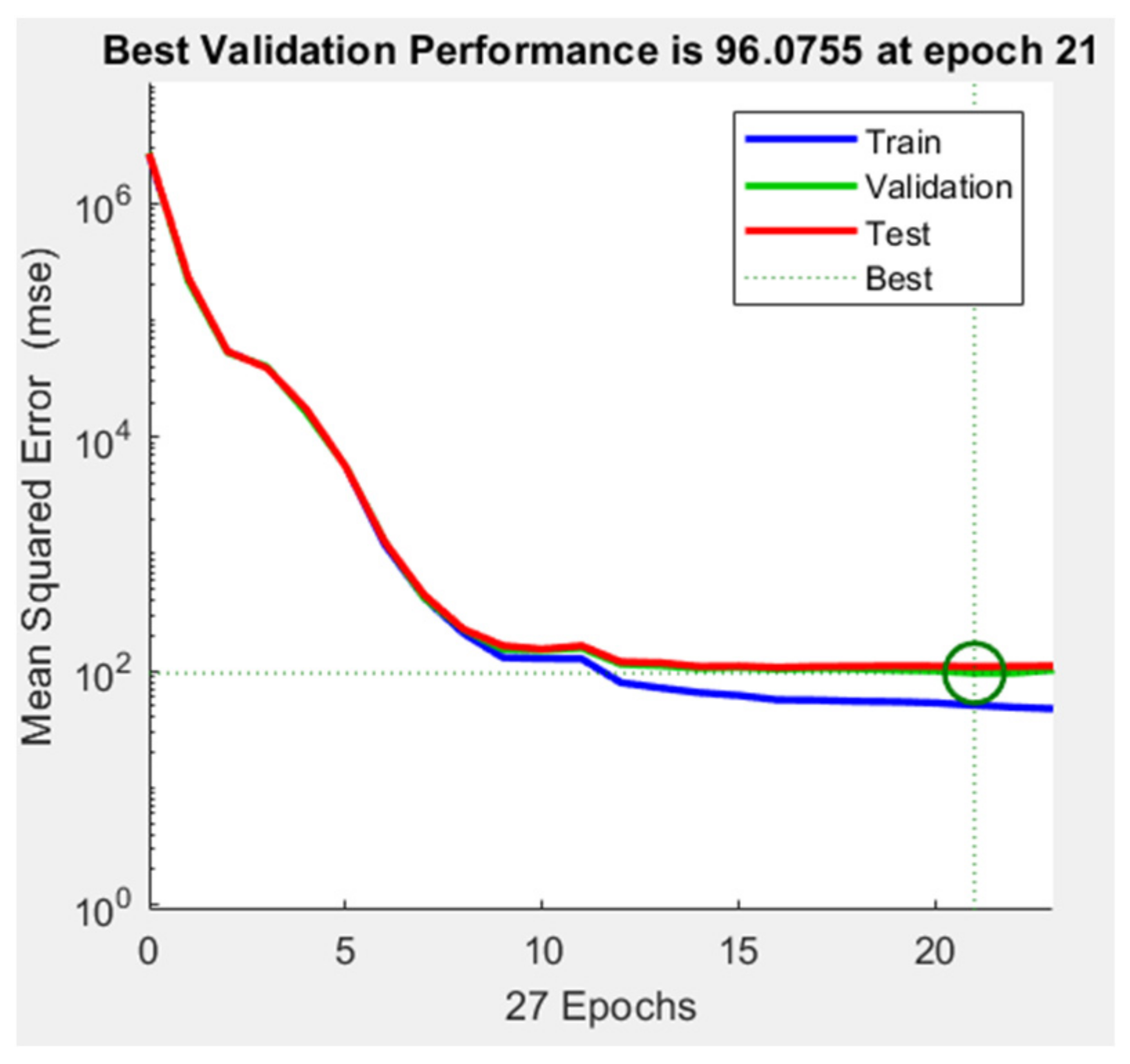
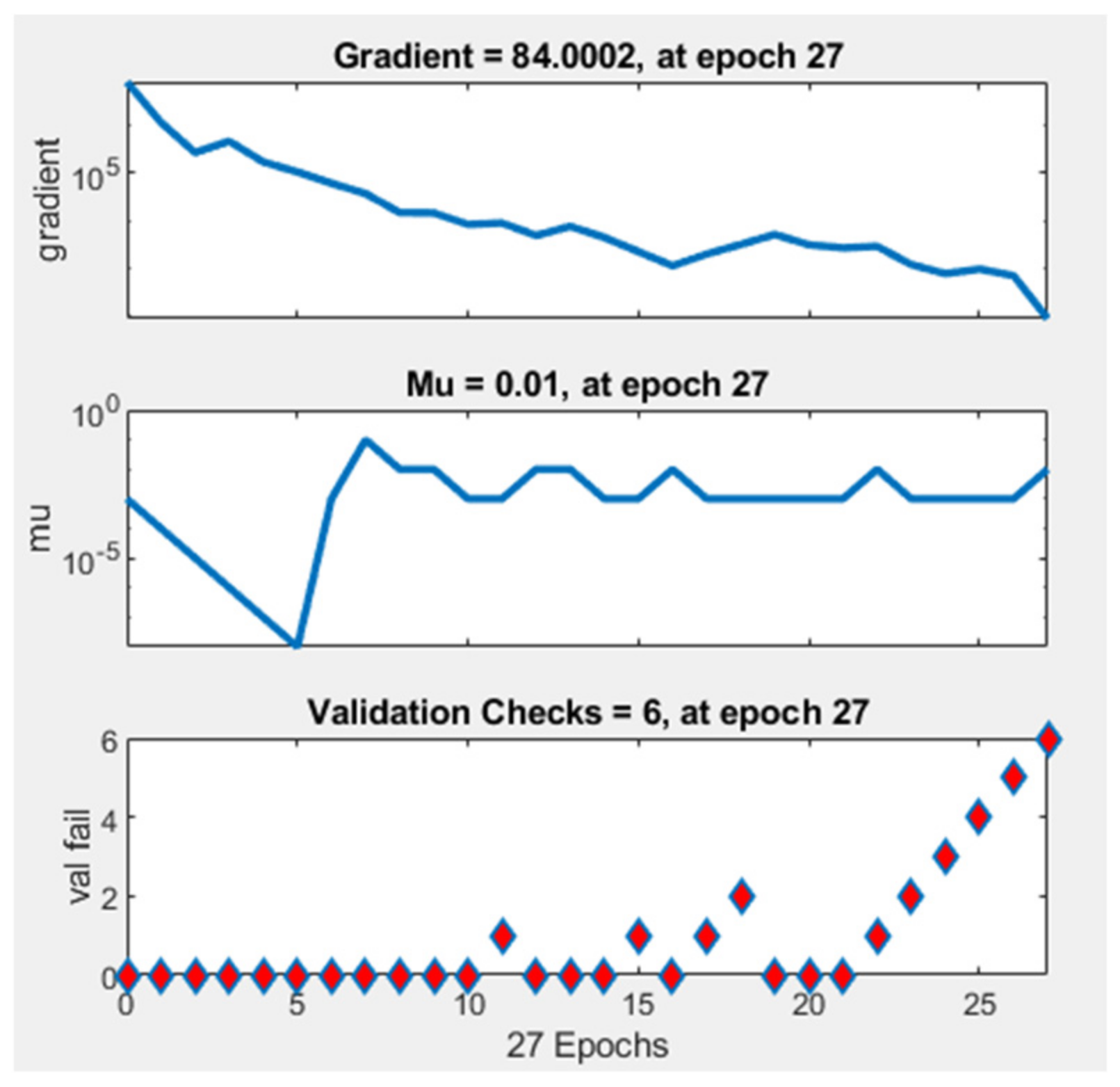
3.2. Artificial Neural Network Model
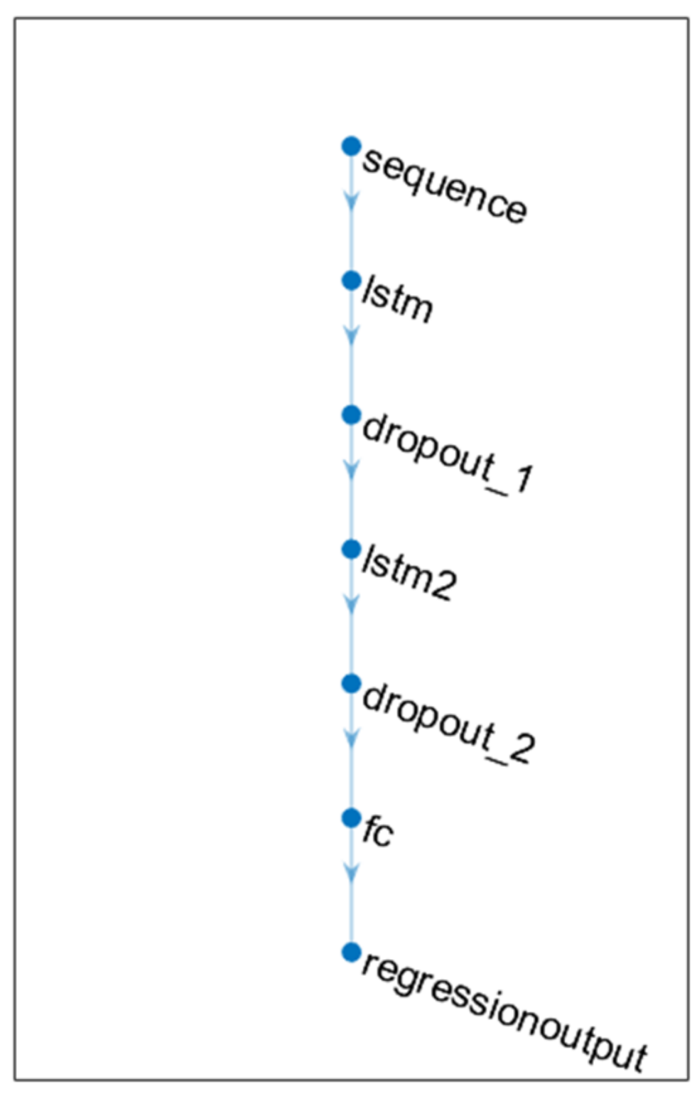
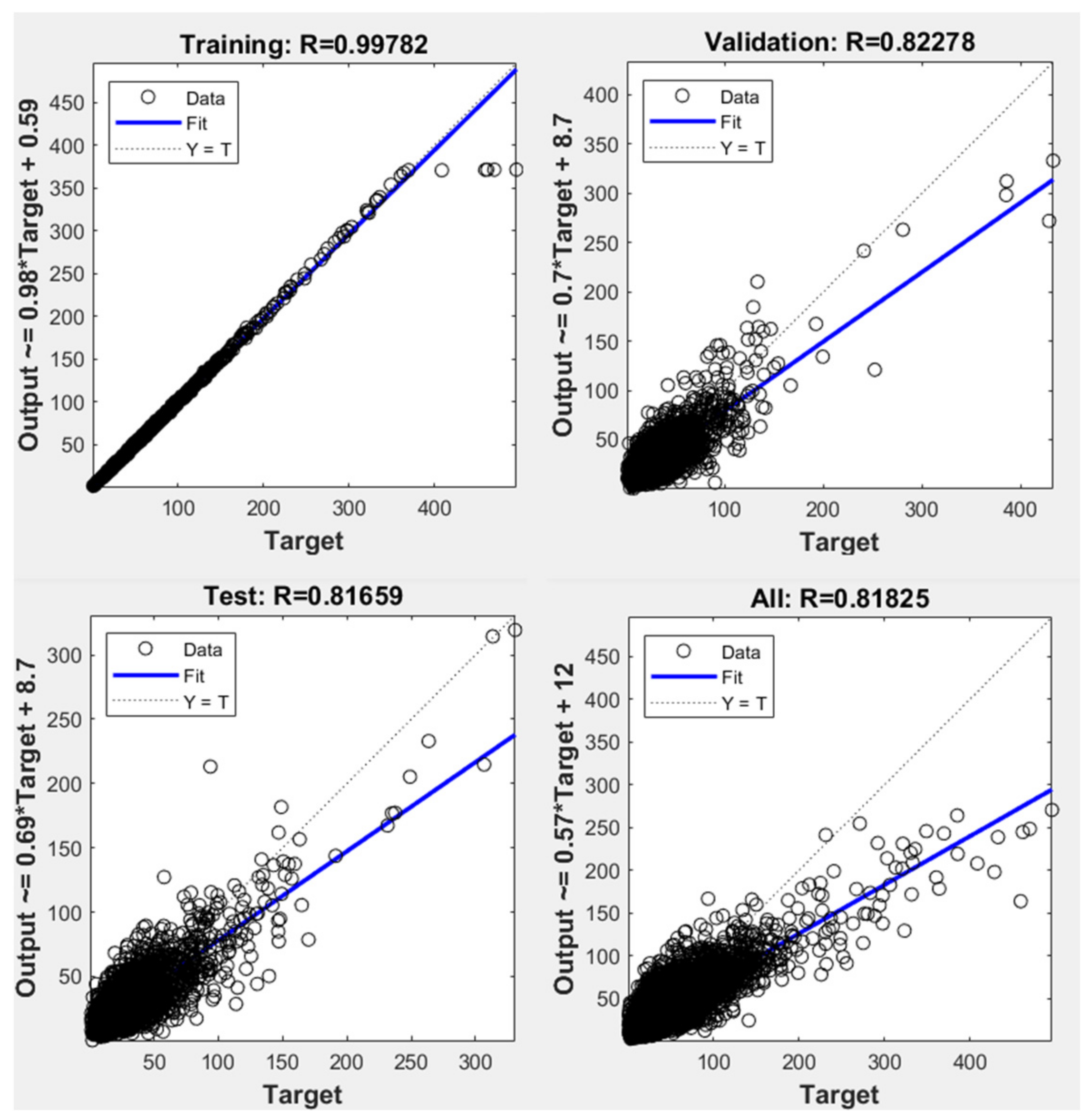
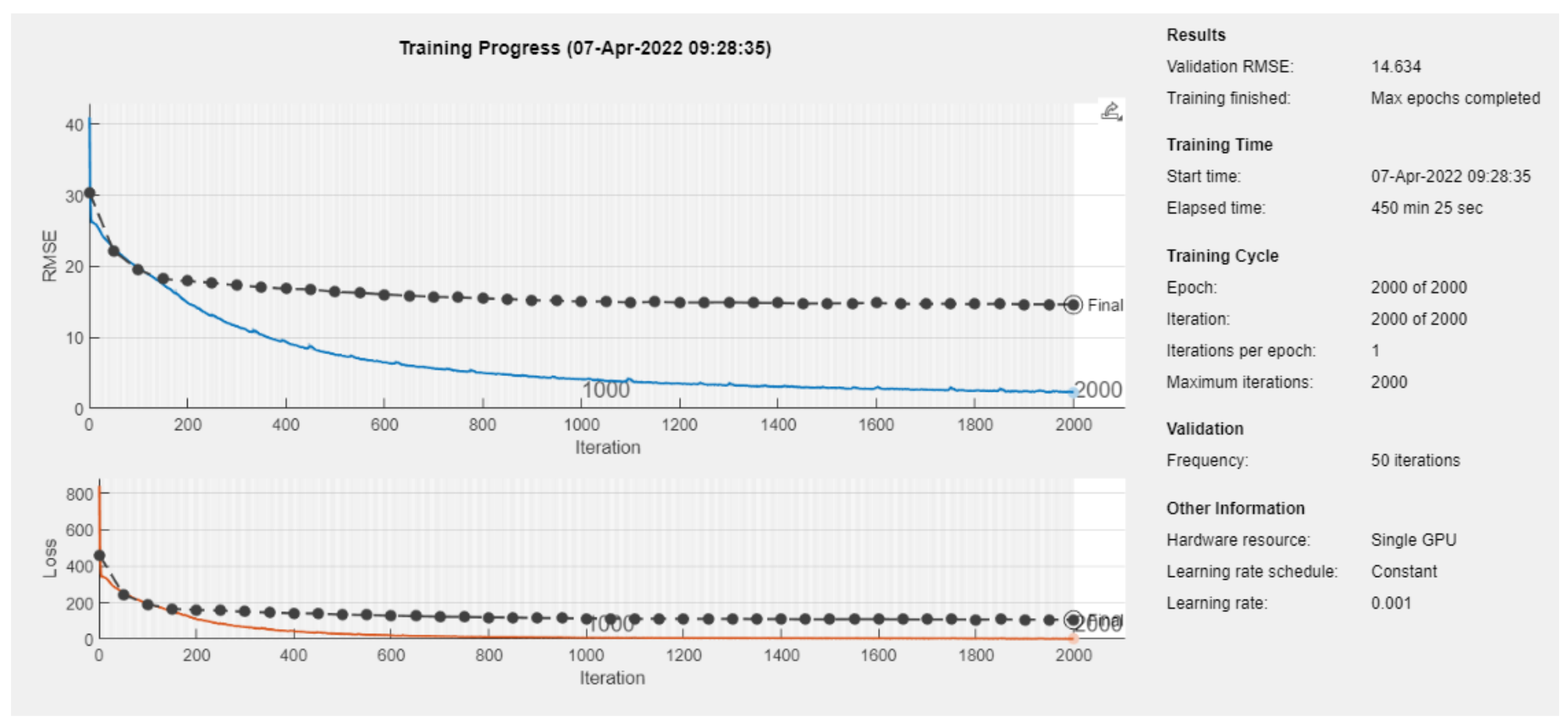
3.3. Long Short-Term Memory Network Model
3.4. Selection of the Best Model
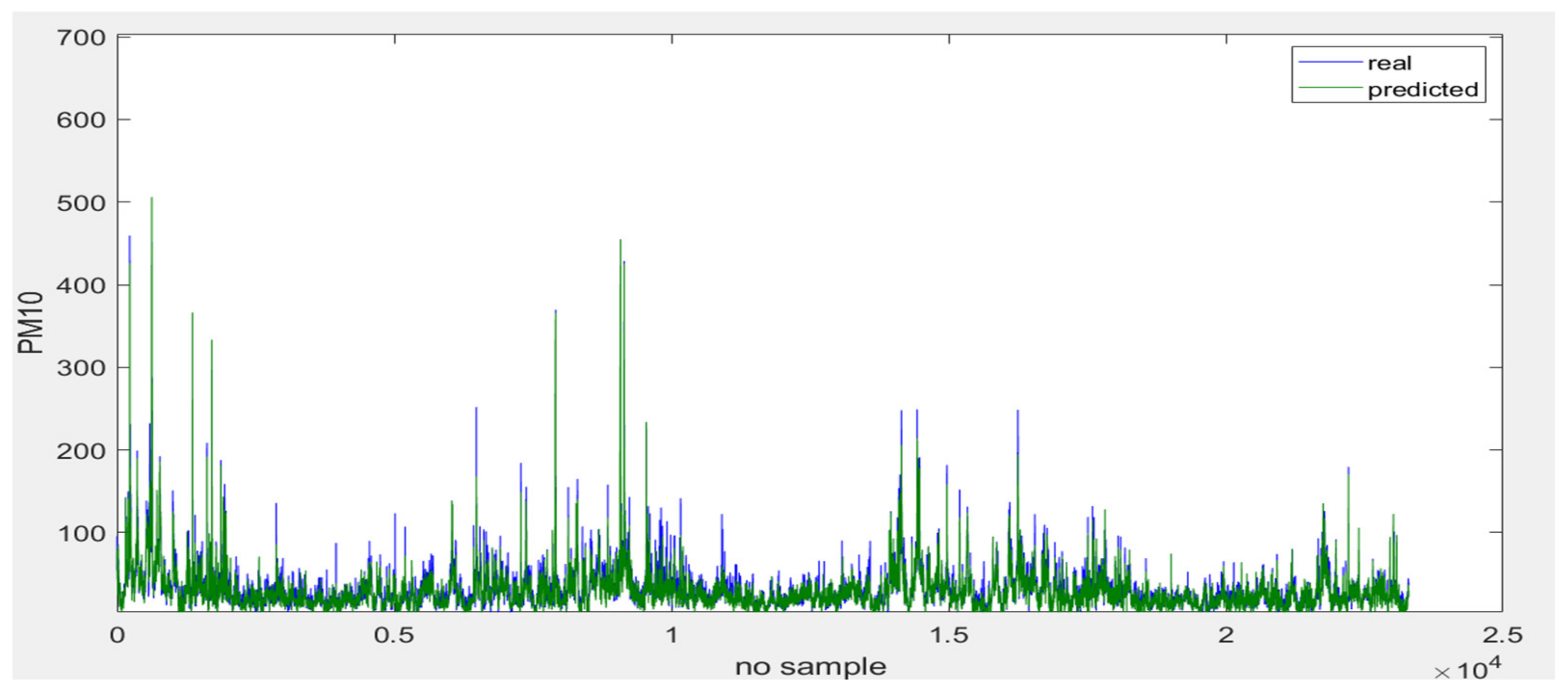
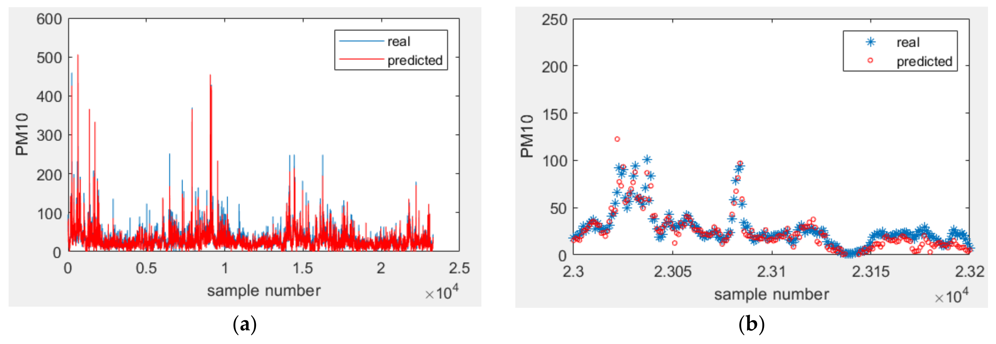
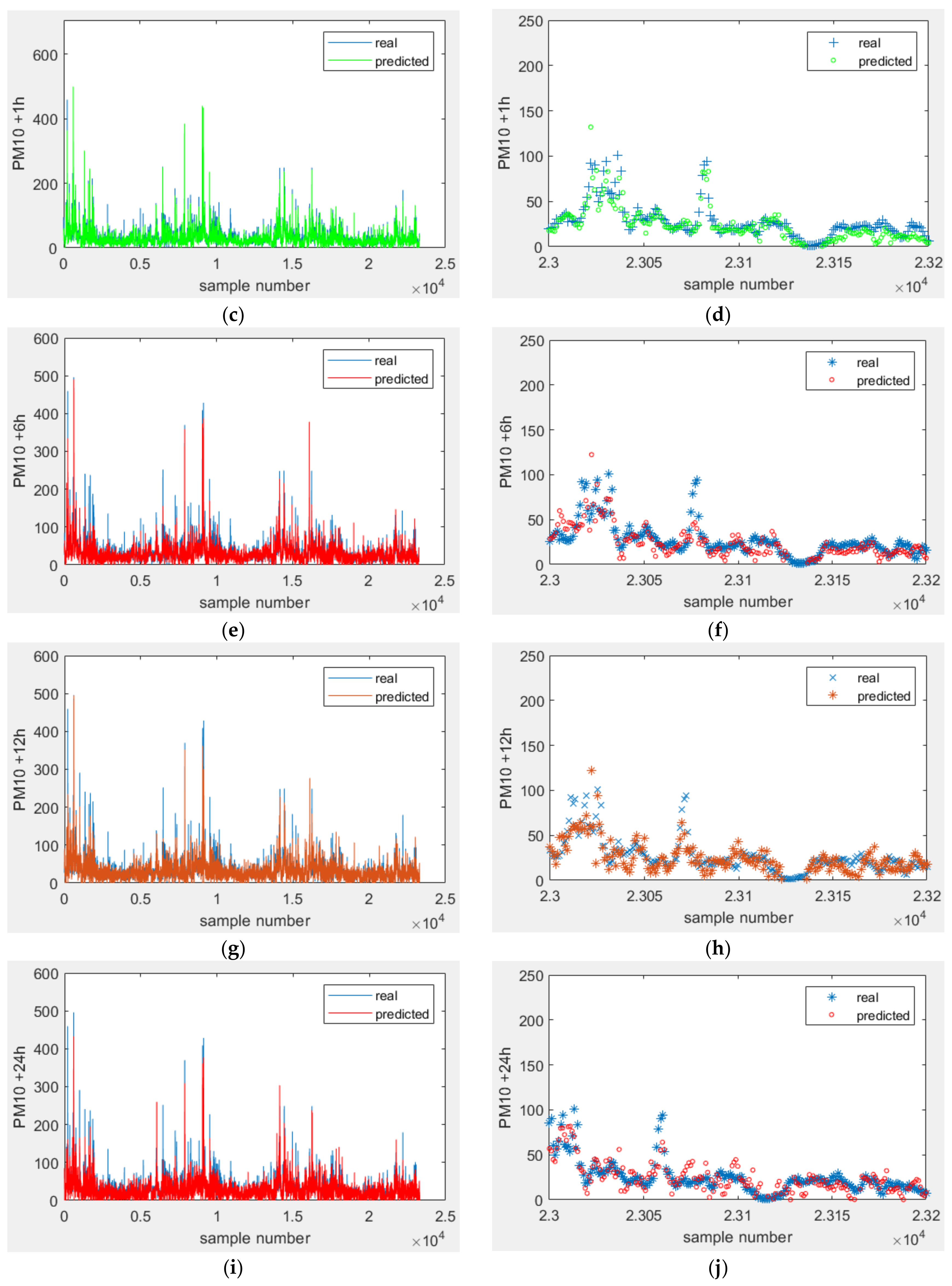
3.5. Prediction Model of Level of PM10 at Different Time Points
4. Discussion

| Year, Place | Model | Type of Input Data | Target | RMSE | R | References |
|---|---|---|---|---|---|---|
| Only winter period (December, January, February) in the period 2002/2003–2016/2021; Gdansk, Gdynia, Sopot, Poland | MLP-ANN | air temperature (AT), relative humidity (RH), air pressure, wind speed (VS) | hourly PM10 concentrations 1–6 h ahead | 9.42–23.56 | 0.50–0.84 | [31] |
| 2009–2017, 6 stations in Ankara | ANN | PM10 | 24-h PM10 concentration | 20.8 | 0.58 | [58] |
| Canetto 2009–2014 | ANN | meteorological variables | 24-h PM10 concentration | - | 0.59 | [59] |
| London, 2007–2012 | ANN | Meteorological variables (wind velocities, wind direction, solar radiation, relative humidity, ambient temperature) and the data type (traffic volume, sound level and speeds) | 24-h PM10 concentration | - | 0.8 | [26] |
| 2020, 28 cities of India, 2016–2018 | MLP–ANN | PM10, WS, RH, AT, CO2, NO2, SO2, Rainfall, Dew point | PM10 for 1 day ahead | - | 0.65 | [60] |
| Kocaeli, Turcja, 120 dni, 2 stacje | ANN | T, RH, AP (hPa), WS direction | PM-10 | - | 0.74 | [61] |
| Delhi, India, May 2016–May 2018 | ANN | PM, CO, SO2, NOx NO, C7H8, NO2, WS, WD (wind direction), VWS (vertical wind speed), RH, Temperature (T), Solar radiation | PM-10 | - | 0.85 | [62] |
| the model presented in the work | ANN | T, RH, WS, WD, and air pollution data were: SO2, PM10, NO2, NOx, CO, O3, C6H6 | PM10 after 1 h, after 6 h, after 12 h and after 24 h | 8.25 | 0.89 |
5. Conclusions
Author Contributions
Funding
Institutional Review Board Statement
Informed Consent Statement
Data Availability Statement
Conflicts of Interest
References
- Połednik, B. Emissions of Air Pollution in Industrial and Rural Region in Poland and Health Impacts. J. Ecol. Eng. 2022, 23, 250–258. [Google Scholar] [CrossRef]
- Millán-Martínez, M.; Sánchez-Rodas, D.; Sánchez de la Campa, A.M.; de la Rosa, J. Impact of the SARS-CoV-2 lockdown measures in Southern Spain on PM10 trace element and gaseous pollutant concentrations. Chemosphere 2022, 303, 134853. [Google Scholar] [CrossRef] [PubMed]
- Manisalidis, I.; Stavropoulou, E.; Stavropoulos, A.; Bezirtzoglou, E. Environmental and Health Impacts of Air Pollution: A Review. Front. Public Health 2020, 8, 14. [Google Scholar] [CrossRef] [PubMed]
- Yousaf, H.S.; Abbas, M.; Ghani, N.; Chaudhary, H.; Fatima, A.; Ahmad, Z.; Yasin, S.A. A comparative assessment of air pollutants of smog in wagah border and other sites in Lahore, Pakistan. Braz. J. Biol. 2021, 84, 1–11. [Google Scholar] [CrossRef]
- Regulation of the Minister of Climate and Environment of 11 December 2020 on Assessing the Levels of Substances in the Air (Journal of Laws 2020, item 2279). Available online: https://isap.sejm.gov.pl/isap.nsf/download.xsp/WDU20010620627/U/D20010627Lj.pdf (accessed on 5 March 2022).
- PN-EN 12341:2014-07; Ambient Air—Standard Gravimetric Measurement Method for the Determination of the PM10 or PM2.5 Mass Concentration of Suspended Particulate Matter. European Standards: Brussels, Belgium, 2014.
- PN-EN 16450:2017-05; Ambient Air—Automated Measuring Systems for the Measurement of the Concentration of Particulate Matter (PM10; PM2.5). European Standards: Brussels, Belgium, 2017.
- Danek, T.; Weglinska, E.; Zareba, M. The influence of meteorological factors and terrain on air pollution concentration and migration: A geostatistical case study from Krakow, Poland. Sci. Rep. 2022, 12, 11050. [Google Scholar] [CrossRef]
- Andrews, B.A. Clean air handbook. Choice Rev. Online 2015, 52, 52–5100. [Google Scholar] [CrossRef]
- Jia, Y.Y.; Wang, Q.; Liu, T. Toxicity research of PM2.5 compositions in vitro. Int. J. Environ. Res. Public Health 2017, 14, 232. [Google Scholar] [CrossRef]
- Sówka, I.; Nych, A.; Kobus, D.; Bezyk, Y.; Zathey, M. Analysis of exposure of inhabitants of Polish cities to air pollution with particulate matters with application of statistical and geostatistical tools. E3S Web. Conf. 2019, 100, 00075. [Google Scholar] [CrossRef]
- Kobus, D.; Merenda, B.; Sówka, I.; Chlebowska-Styś, A.; Wroniszewska, A. Ambient air quality as a condition of effective healthcare therapy on the example of selected polish health resorts. Atmosphere 2020, 11, 882. [Google Scholar] [CrossRef]
- Klimont, Z.; Kupiainen, K.; Heyes, C.; Purohit, P.; Cofala, J.; Rafaj, P.; Borken-Kleefeld, J.; Schöpp, W. Global anthropogenic emissions of particulate matter including black carbon. Atmos. Chem. Phys. 2017, 17, 8681–8723. [Google Scholar] [CrossRef] [Green Version]
- Directive 2008/50/EC of the European Parliament and of the Council of 21 May 2008 on Ambient Air Quality and Cleaner Air for Europe. Available online: http://eur-lex.europa.eu/legal-content/en/ALL/?uri=CELEX:32008L0050 (accessed on 5 March 2022).
- Ordieres, J.B.; Vergara, E.P.; Capuz, R.S.; Salazar, R.E. Neural network prediction model for fine particulate matter (PM 2.5) on the US-Mexico border in El Paso (Texas) and Ciudad Juárez (Chihuahua). Environ. Model. Softw. 2005, 20, 547–559. [Google Scholar] [CrossRef]
- The National Centre for Emissions Management (KOBiZE). Available online: https://kobize.pl/en/page/id/409/about-us (accessed on 5 March 2022).
- Chief Inspectorate of Environmental Protection (GIOŚ in Polish) Report on the Forecast of PM2.5 and PM10 Concentrations for 2020 and 2025. 2020. Available online: https://www.lubelskie.pl/file/2020/08/POP_strefa_Aglomeracja_Lubelska_0601.pdf (accessed on 5 March 2022).
- The Lublin Regional Assembly Air Protection in Lublin Agglomeration. 2020. Available online: https://edziennik.lublin.uw.gov.pl/legalact/2020/4028/ (accessed on 5 March 2022).
- The Act of 27 April 2001, Environmental Protection Law (Journal of Laws of 2020, item 1219, as Amended). Available online: https://isap.sejm.gov.pl/isap.nsf/download.xsp/WDU20081991227/U/D20081227Lj.pdf (accessed on 5 March 2022).
- Łobocki, L. Methodological Guidelines for Mathematical Modeling in the Air Quality Management System. Available online: https://www.mos.gov.pl/kategoria/2135_wskazowki_metodyczne_dotyczace_modelowania_matematycznego_w_systemie_zarzadzania_jakoscia_powietrza/ (accessed on 5 March 2022).
- Institute of Meteorology and Water Management—National Research Institute. Available online: https://imgw.pl/ (accessed on 5 March 2022).
- Baklanov, A.; Zhang, Y. Advances in air quality modeling and forecasting. Glob. Transit. 2020, 2, 261–270. [Google Scholar] [CrossRef]
- Lu, W.-Z.; Wang, W.-J.; Wang, X.-K.; Yan, S.-H.; Lam, J.C. Potential assessment of a neural network model with PCA/RBF approach for forecasting pollutant trends in Mong Kok urban air, Hong Kong. Environ. Res. 2004, 96, 79–87. [Google Scholar] [CrossRef]
- Azid, A.; Juahir, H.; Toriman, M.E.; Kamarudin, M.K.A.; Saudi, A.S.M.; Hasnam, C.N.C.; Aziz, N.A.A.; Azaman, F.; Latif, M.T.; Zainuddin, S.F.M.; et al. Prediction of the level of air pollution using principal component analysis and artificial neural network techniques: A case study in Malaysia. Water Air Soil Pollut. 2014, 225, 2063. [Google Scholar] [CrossRef]
- Arhami, M.; Kamali, N.; Rajabi, M.M. Predicting hourly air pollutant levels using artificial neural networks coupled with uncertainty analysis by Monte Carlo simulations. Environ. Sci. Pollut. Res. 2013, 20, 4777–4789. [Google Scholar] [CrossRef]
- Suleiman, A.; Tight, M.R.; Quinn, A.D. Applying machine learning methods in managing urban concentrations of traffic-related particulate matter (PM10 and PM2.5). Atmos. Pollut. Res. 2019, 10, 134–144. [Google Scholar] [CrossRef]
- Mehdipour, V.; Stevenson, D.S.; Memarianfard, M.; Sihag, P. Comparing different methods for statistical modeling of particulate matter in Tehran, Iran. Air Qual. Atmos. Health 2018, 11, 1155–1165. [Google Scholar] [CrossRef]
- Krishan, M.; Jha, S.; Das, J.; Singh, A.; Goyal, M.K.; Sekar, C. Air quality modelling using long short-term memory (LSTM) over NCT-Delhi, India. Air Qual. Atmos. Health 2019, 12, 899–908. [Google Scholar] [CrossRef]
- Cai, M.; Yin, Y.; Xie, M. Prediction of hourly air pollutant concentrations near urban arterials using artificial neural network approach. Transp. Res. Part D Transp. Environ. 2009, 14, 32–41. [Google Scholar] [CrossRef]
- Mao, W.; Wang, W.; Jiao, L.; Zhao, S.; Liu, A. Modeling air quality prediction using a deep learning approach: Method optimization and evaluation. Sustain. Cities Soc. 2021, 65, 102567. [Google Scholar] [CrossRef]
- Nidzgorska-Lencewicz, J. Application of artificial neural networks in the prediction of PM10 levels in thewinter months: A case study in the Tricity Agglomeration, Poland. Atmosphere 2018, 9, 203. [Google Scholar] [CrossRef]
- Czernecki, B.; Marosz, M.; Jędruszkiewicz, J. Assessment of machine learning algorithms in short-term forecasting of pm10 and pm2.5 concentrations in selected polish agglomerations. Aerosol Air Qual. Res. 2021, 21, 200586. [Google Scholar] [CrossRef]
- Matlab R2022a The MathWorks, Inc., Natick, MA, USA. Available online: https://matlab.mathworks.com/ (accessed on 10 March 2022).
- R 4.1.2 R Foundation for Statistical Computing, Vienna, Austria. Available online: http://www.r-project.org/index.html (accessed on 10 March 2022).
- Elsheikh, A.H.; Sharshir, S.W.; Elaziz, M.A.; Kabeel, A.E.; Guilan, W.; Haiou, Z. Modeling of solar energy systems using artificial neural network: A comprehensive review. Sol. Energy 2021, 149, 223–233. [Google Scholar] [CrossRef]
- Chu, H.; Wei, J.; Wu, W. Streamflow prediction using LASSO-FCM-DBN approach based on hydro-meteorological condition classification. J. Hydrol. 2020, 580, 124253. [Google Scholar] [CrossRef]
- Son, Y.; Osornio-Vargas, Á.R.; O’Neill, M.S.; Hystad, P.; Texcalac-Sangrador, J.L.; Ohman-Strickland, P.; Meng, Q.; Schwander, S. Land use regression models to assess air pollution exposure in Mexico City using finer spatial and temporal input parameters. Sci. Total Environ. 2018, 639, 40–48. [Google Scholar] [CrossRef] [PubMed]
- Xu, G.; Ren, X.; Xiong, K.; Li, L.; Bi, X.; Wu, Q. Analysis of the driving factors of PM2.5 concentration in the air: A case study of the Yangtze River Delta, China. Ecol. Indic. 2020, 110, 105889. [Google Scholar] [CrossRef]
- Fan, W.; Si, F.; Ren, S.; Yu, C.; Cui, Y.; Wang, P. Integration of continuous restricted Boltzmann machine and SVR in NOx emissions prediction of a tangential firing boiler. Chemom. Intell. Lab. Syst. 2019, 195, 103870. [Google Scholar] [CrossRef]
- Murillo-Escobar, J.; Sepulveda-Suescun, J.P.; Correa, M.A.; Orrego-Metaute, D. Forecasting concentrations of air pollutants using support vector regression improved with particle swarm optimization: Case study in Aburrá Valley, Colombia. Urban Clim. 2019, 29, 100473. [Google Scholar] [CrossRef]
- Saxena, A.; Shekhawat, S. Ambient Air Quality Classification by Grey Wolf Optimizer Based Support Vector Machine. J. Environ. Public Health 2017, 2017. [Google Scholar] [CrossRef]
- Zhu, S.; Lian, X.; Wei, L.; Che, J.; Shen, X.; Yang, L.; Qiu, X.; Liu, X.; Gao, W.; Ren, X.; et al. PM2.5 forecasting using SVR with PSOGSA algorithm based on CEEMD, GRNN and GCA considering meteorological factors. Atmos. Environ. 2018, 183, 20–32. [Google Scholar] [CrossRef]
- Kamińska, J.A. The use of random forests in modelling short-term air pollution effects based on traffic and meteorological conditions: A case study in Wrocław. J. Environ. Manag. 2018, 217, 164–174. [Google Scholar] [CrossRef]
- Rubal; Kumar, D. Evolving Differential evolution method with random forest for prediction of Air Pollution. Procedia Comput. Sci. 2018, 132, 824–833. [Google Scholar] [CrossRef]
- Sun, H.; Gui, D.; Yan, B.; Liu, Y.; Liao, W.; Zhu, Y.; Lu, C.; Zhao, N. Assessing the potential of random forest method for estimating solar radiation using air pollution index. Energy Convers. Manag. 2016, 119, 121–129. [Google Scholar] [CrossRef]
- Wang, Y.; Du, Y.; Wang, J.; Li, T. Calibration of a low-cost PM2.5 monitor using a random forest model. Environ. Int. 2019, 133, 105161. [Google Scholar] [CrossRef]
- Wen, C.; Liu, S.; Yao, X.; Peng, L.; Li, X.; Hu, Y.; Chi, T. A novel spatiotemporal convolutional long short-term neural network for air pollution prediction. Sci. Total Environ. 2019, 654, 1091–1099. [Google Scholar] [CrossRef]
- Rahman, M.M.; Shafiullah, M.; Rahman, S.M.; Khondaker, A.N.; Amao, A.; Zahir, M.H. Soft computing applications in air quality modeling: Past, present, and future. Sustainability 2020, 12, 4045. [Google Scholar] [CrossRef]
- Lu, H.C. The statistical characters of PM10 concentration in Taiwan area. Atmos. Environ. 2002, 36, 491–502. [Google Scholar] [CrossRef]
- Kim, M.J.; Yun, J.P.; Yang, J.B.R.; Choi, S.J.; Kim, D. Prediction of the temperature of liquid aluminum and the dissolved hydrogen content in liquid aluminum with a machine learning approach. Metals 2020, 10, 330. [Google Scholar] [CrossRef]
- Shahriar, S.A.; Kayes, I.; Hasan, K.; Salam, M.A.; Chowdhury, S. Applicability of machine learning in modeling of atmospheric particle pollution in Bangladesh. Air Qual. Atmos. Health 2020, 13, 1247–1256. [Google Scholar] [CrossRef]
- Jang, J.; Shin, S.; Lee, H.; Moon, I.C. Forecasting the concentration of particulate matter in the seoul metropolitan area using a gaussian process model. Sensors 2020, 20, 3845. [Google Scholar] [CrossRef]
- Brusca, S.; Famoso, F.; Lanzafame, R.; Mauro, S.; Messina, M.; Strano, S. PM10 Dispersion Modeling by Means of CFD 3D and Eulerian-Lagrangian Models: Analysis and Comparison with Experiments. Energy Procedia 2016, 101, 329–336. [Google Scholar] [CrossRef]
- Elsheikh, A.H.; Saba, A.I.; Elaziz, M.A.; Lu, S.; Shanmugan, S.; Muthuramalingam, T.; Kumar, R.; Mosleh, A.O.; Essa, F.A.; Shehabeldeen, T.A. Deep learning-based forecasting model for COVID-19 outbreak in Saudi Arabia. Process Saf. Environ. Prot. 2021, 149, 223–233. [Google Scholar] [CrossRef] [PubMed]
- Hu, C.; Wu, Q.; Li, H.; Jian, S.; Li, N.; Lou, Z. Deep learning with a long short-term memory networks approach for rainfall-runoff simulation. Water 2018, 10, 1543. [Google Scholar] [CrossRef]
- Voukantsis, D.; Karatzas, K.; Kukkonen, J.; Räsänen, T.; Karppinen, A.; Kolehmainen, M. Intercomparison of air quality data using principal component analysis, and forecasting of PM10 and PM2.5 concentrations using artificial neural networks, in Thessaloniki and Helsinki. Sci. Total Environ. 2011, 409, 1266–1276. [Google Scholar] [CrossRef]
- Kowalski, P.; Warchalowski, W. The comparison of linear models for PM10 and PM2.5 forecasting. WIT Trans. Ecol. Environ. 2018, 230, 177–187. [Google Scholar] [CrossRef]
- Bozdağ, A.; Dokuz, Y.; Gökçek, Ö.B. Spatial prediction of PM10 concentration using machine learning algorithms in Ankara, Turkey. Environ. Pollut. 2020, 263, 114635. [Google Scholar] [CrossRef]
- Tamas, W.; Notton, G.; Paoli, C.; Nivet, M.L.; Voyant, C. Hybridization of air quality forecasting models using machine learning and clustering: An original approach to detect pollutant peaks. Aerosol Air Qual. Res. 2016, 16, 405–416. [Google Scholar] [CrossRef]
- Dutta, A.; Jinsart, W. Air Pollution in Indian Cities and Comparison of MLR, ANN and CART Models for Predicting PM10 Concentrations in Guwahati, India. Asian J. Atmos. Environ. 2021, 15, 2020131. [Google Scholar] [CrossRef]
- Özdemir, U.; Taner, S. Impacts of Meteorological Factors on PM10: Artificial Neural Networks (ANN) and Multiple Linear Regression (MLR) Approaches. Environ. Forensics 2014, 15, 329–336. [Google Scholar] [CrossRef]
- Masood, A.; Ahmad, K. A model for particulate matter (PM2.5) prediction for Delhi based on machine learning approaches. Procedia Comput. Sci. 2020, 167, 2101–2110. [Google Scholar] [CrossRef]


| Minimum | Maximum | Mean | Standard Deviation | Skewness | Kurtosis | |
|---|---|---|---|---|---|---|
| SO2 | 0 | 56.9 | 4.93 | 3.47 | 3.13 | 20.13 |
| PM10 | 0.5 | 496 | 30.95 | 25.94 | 4.79 | 46.67 |
| NO2 | 0 | 128.2 | 21.07 | 15.21 | 1.77 | 4.23 |
| NOx | 0 | 766.7 | 32.21 | 39.79 | 6.52 | 70.76 |
| CO | 0 | 5.32 | 0.36 | 0.3 | 4.76 | 41.40 |
| O3 | 0 | 169.6 | 48.88 | 28.31 | 0.41 | −0.30 |
| C6H6 | 0.05 | 25.3 | 1.69 | 1.5 | 4.52 | 42.40 |
| T | −15.34 | 36.84 | 10.22 | 9.37 | 0.10 | −0.85 |
| RH | 21 | 100 | 72.39 | 18.51 | −0.44 | −0.95 |
| WS | 0 | 20.67 | 5.21 | 2.87 | 1.19 | 1.75 |
| WD | 0.65 | 360 | 196.66 | 94.99 | −0.28 | −0.99 |
| Methods | Model Parameters |
|---|---|
| K-Nearest Neighbor Regression (KNNR) | The dataset was normalized and the Euclidean distance was used to find the closest neighbors, k = 1, 2, …, 10 were tested. |
| Support Vector Machine (SVM) | Various Kernel functions were employed for training SVM: Gaussian kernel, Linear kernel, Quadratic kernel, Cubic kernel. Kernel scale, box constraint, epsilon—Automatic, standardize data: true. |
| Regression Trees (RT) | Minimum leaf size setting was changed while training RT. The analysis was conducted using Minimum leaf size—4, 12 and 36. Surrogate decision splits—Off. |
| Gaussian Process Regression Models (GPR) | GPR was trained using various Kernel functions: Rational Quadratic, Squared Exponential, Matern 5/2 and Exponential. Hyperparameters: basis function: Zero, Constant and Linear, use isotropic kernel: true, kernel scale, signal standard deviation and sigma: Automatic, standardize, optimize numeric parameters: true |
| Artificial Neural Network (ANN) | Three different algorithms were used to train the network: the Levenberg–Marquardt algorithm, Bayesian regularization algorithm and Scaled conjugate gradient algorithm. The number of neurons in the hidden layer (10–300) was selected experimentally. In this case, the learning set was 70%, whereas the test and validation sets were 15% each. Networks were built with one hidden layer. |
| Long Short-Term Memory network (LSTM) | To teach the network, the number of hidden units was experimentally selected in the range of 500 to 2000. Solver for training network—‘Adam’, dropout layers—0.2, mini-batch size—changed in the range of 500–1000, option to pad, truncate, or split input sequences, specified as longest. The learning set for this network was 70%, and the test and validation sets were 15% each. |
| Model Quality Parameters | Models Obtained Using Machine Learning Methods | ||||
|---|---|---|---|---|---|
| LR | KNNR | SVM | RT | GPR | |
| R2 | 0.8 | 0.79 | 0.82 | 0.77 | 0.89 |
| MSE | 135.51 | 135.24 | 119.3 | 156.57 | 85.36 |
| Unit | Initial Value | Stopped Value | Target Value |
|---|---|---|---|
| Epoch | 0 | 27 | 1000 |
| Elapsed Time | - | 00:06:49 | - |
| Performance | 2.63 × 10⁶ | 44.9 | 0 |
| Gradient | 8.39 × 10⁶ | 84 | 1 × 10⁻⁷ |
| Mu | 0.001 | 0.01 | 1 × 10¹⁰ |
| Validation Checks | 0 | 6 | 6 |
| Observations | MSE | R | R2 | |
|---|---|---|---|---|
| Training | 16,310 | 50.93 | 0.96 | 0.92 |
| Validation | 3495 | 96.07 | 0.94 | 0.86 |
| Test | 3495 | 109.11 | 0.92 | 0.83 |
| Observations | MSE | R | R2 | |
|---|---|---|---|---|
| Training | 16,310 | 3.1 | 0.99 | 0.99 |
| Validation | 3495 | 214.14 | 0.82 | 0.67 |
| Test | 3495 | 206.17 | 0.81 | 0.66 |
| Quality Parameter | Models Obtained Using Machine Learning Methods | ANN | LSTM | ||||
|---|---|---|---|---|---|---|---|
| LR | KNNR | SVM | RT | GPR | |||
| R2 | 0.8 | 0.79 | 0.82 | 0.77 | 0.89 | 0.90 | 0.82 |
| MSE | 135.51 | 135.24 | 119.3 | 156.57 | 85.36 | 68.09 | 233.52 |
| RMSE | 11.64 | 11.62 | 10.92 | 12.51 | 9.24 | 8.25 | 15.28 |
| MAE | 8.06 | 8.02 | 7.13 | 8.25 | 6.12 | 5.44 | 9.93 |
| Models Obtained Using Machine Learning Methods | ANN | LSTM | |||||
|---|---|---|---|---|---|---|---|
| LR | KNNR | SVM | RT | GPR | |||
| Training time [min] | 10:05 | 00:06 | 65:11 | 10:38 | 129:42 | 06:49 | 450:25 |
| Prediction speed [obs/s] | 34,000 | 3380 | 12,000 | 78,000 | 1400 | 94,000 | 1500 |
| Unit | Initial Value | Stopped Value | Target Value |
|---|---|---|---|
| Epoch | 0 | 28 | 1000 |
| Elapsed Time | - | 04:15:51 | - |
| Performance | 5.76 × 10⁶ | 82.8 | 0 |
| Gradient | 8.75 × 10⁶ | 504 | 1 × 10⁻⁷ |
| Mu | 0.001 | 0.01 | 1 × 10¹⁰ |
| Validation Checks | 0 | 6 | 6 |
| Observations | MSE | R | |
|---|---|---|---|
| Training | 16,310 | 91.24 | 0.92 |
| Validation | 3495 | 271.94 | 0.80 |
| Test | 3495 | 225.72 | 0.83 |
Publisher’s Note: MDPI stays neutral with regard to jurisdictional claims in published maps and institutional affiliations. |
© 2022 by the authors. Licensee MDPI, Basel, Switzerland. This article is an open access article distributed under the terms and conditions of the Creative Commons Attribution (CC BY) license (https://creativecommons.org/licenses/by/4.0/).
Share and Cite
Kujawska, J.; Kulisz, M.; Oleszczuk, P.; Cel, W. Machine Learning Methods to Forecast the Concentration of PM10 in Lublin, Poland. Energies 2022, 15, 6428. https://doi.org/10.3390/en15176428
Kujawska J, Kulisz M, Oleszczuk P, Cel W. Machine Learning Methods to Forecast the Concentration of PM10 in Lublin, Poland. Energies. 2022; 15(17):6428. https://doi.org/10.3390/en15176428
Chicago/Turabian StyleKujawska, Justyna, Monika Kulisz, Piotr Oleszczuk, and Wojciech Cel. 2022. "Machine Learning Methods to Forecast the Concentration of PM10 in Lublin, Poland" Energies 15, no. 17: 6428. https://doi.org/10.3390/en15176428
APA StyleKujawska, J., Kulisz, M., Oleszczuk, P., & Cel, W. (2022). Machine Learning Methods to Forecast the Concentration of PM10 in Lublin, Poland. Energies, 15(17), 6428. https://doi.org/10.3390/en15176428