Article

Model Predictive Control for Photovoltaic Plants with Non-Ideal Energy Storage Using Mixed Integer Linear Programming

1
Departamento Electrónica, Universidad Técnica Federico Santa María (UTFSM), Av. España 1680, Valparaíso 2390123, Chile
2
Advanced Center for Electrical and Electronic Engineering (AC3E), Gral. Bari 699, Valparaíso 2390136, Chile
3
Centro Científico Tecnológico de Valparaíso (CCTVal), Gral. Bari 699, Valparaíso 2390136, Chile
*
Author to whom correspondence should be addressed.
Energies 2022, 15(17), 6427; https://doi.org/10.3390/en15176427
Submission received: 3 August 2022 / Revised: 30 August 2022 / Accepted: 31 August 2022 / Published: 2 September 2022
(This article belongs to the Section D: Energy Storage and Application)

Abstract

:
This paper proposes a model-based predictive control strategy based on mixed-integer linear programming for a photovoltaic power plant with battery energy storage. The control objective is to maximize the revenues from energy delivered from both photovoltaic panels and batteries to the grid in a deregulated electricity market. For each control interval, the proposed algorithm incorporates information on solar radiation, market prices, and the state of charge of the batteries to determine the intervals of energy injection into the grid to maximize the economic benefits. The proposed strategy considers the rate-based variable efficiency in the battery model and time-varying energies prices, thus providing a more general implementation than previous schemes proposed in the literature for the same purpose. Simulations considering the operational procedures of the Spanish market as a case study show that, by integrating the battery efficiency in the model, the proposed control strategy increments the economic benefits in 21% compared to previous results reported in the literature for the same operational conditions. Additionally, the proposed approach reduces the number of charge and discharge cycles, potentially extending the lifespan of batteries.

1. Introduction

Electricity generated from large-scale photovoltaic (PV) plants currently represents a significant part of the total generation in many countries. The proliferation of PV plants has been particularly prominent in regions with high solar irradiance, such as eastern Turkey [1] and northern Chile [2]; however, technological advances such as solar trackers for PV panels can improve the performance of PV systems and help on expanding PV generation to regions with less favorable irradiance conditions [3]. From an economic perspective, PV plants have become attractive not only in energy markets with feed-in tariffs such as Iran [4], but also in deregulated energy markets such as Spain [5,6].
In the deregulated Spanish market, electricity is traded in regular settlement periods, during which participating energy producers commit to delivering a certain amount of energy for future periods in hour blocks. The energy commitment price for each block is settled as pay-as-cleared before the actual time of delivery. At the time of delivery, i.e., in real-time, the power produced by a given generator may deviate from the plan considered at the moment of commitment due to unforeseen contingencies or variations with respect to the forecast of energy production considered during the settlement period. Producers failing to deliver the committed energy may generate a net imbalance in the system. System regulators must cover this imbalance by buying energy available from other generators participating in the market [7]. Energy bought to cover an imbalance is paid at an imbalance price, which is higher than the settled price agreed to in advance for the same block, and it is charged to the market participants that are generating the imbalance via a penalty. Therefore, system imbalances are economically detrimental for producers unable to fulfill their commitment and beneficial for producers with surplus energy available for selling at the time of the imbalance [8].
The variable nature of solar irradiation during a day prevents PV plants from providing a constant power supply [9]. Therefore, it is difficult to guarantee a constant energy delivery for a block of several hours without the risk of breaching this commitment. A typical solution for this issue is integrating battery energy storage systems (BESS), which enable energy accumulation during periods in which real-time production is higher than the commitment. The battery storage, can be of different technologies and be integrated into the PV system either in DC or AC side, with AC coupling being easier to use in retrofit projects and providing higher flexibility during operation [10]. On the other hand, lithium-ion batteries are considered more suitable for market-oriented applications [11,12]. Other applications include the suppression of power fluctuations according to the grid codes’ requirements [13], frequency regulation [14] or integration of different renewable energy sources [15,16].
The energy accumulated in the batteries can be, in turn, delivered to the system during periods in which the real-time energy production from the PV panels is lower than the committed energy. Moreover, producers can sell energy stored in the battery at a higher imbalance price. Considering that the price of committed energy, imbalance price, and the penalties vary for each settlement period, the energy stored in the batteries will have a dynamic relative value, and then the profits obtained by PV energy producers will depend on the adequate choice of intervals to charge or discharge the batteries. Therefore, to maximize the economic benefits obtained from PV plants, producers must implement optimized control strategies to manage the state of charge (SoC) in real-time, considering forecasts of both PV production and energy prices in the corresponding electricity market [14,17].
Multiple authors have tackled the problem of maximizing profits from photovoltaic power plant with battery energy storage system (PV+BESS) in deregulated electricity markets using Model Predictive Control (MPC) [6,16,18]. MPC strategies use prediction models of the system and operational variables to decide the times to charge or discharge the batteries considering estimations of future energy generation and market prices. To this end, MPC schemes must optimize a cost function subject to operational constraints at each sampling interval [19,20]. In our target application, battery efficiency and sometimes market prices are modeled as piece-wise functions, which naturally lead to a Mixed-Integer Linear Programming (MILP) formulation for the optimization problem.
In [6], the authors formulate an optimization problem to maximize profits from a PV+BESS plant in the Spanish market. In this case, the cost function depends on the imbalance price and penalty, which have a piece-wise representation that leads to an MILP formulation. Authors argue that solving an MILP problem in each control interval is computationally prohibitive for real-time operation, and thus they apply ad hoc heuristics to derive an equivalent LP formulation, showing the effectiveness of the control approach using simulations that consider a sampling time of four minutes. Although effective for incrementing profits, authors only consider a simplified model for the battery that omits the piece-wise function that represents the charging and discharging efficiency, which we argue is a relevant aspect for accurate decision-making to maximize profits from energy sales. The work in [18] proposes an MPC scheme for a PV+BESS system operating in the PJM Energy Market (www.pjm.com, accessed on 30 August 2022) with a price scheme that results in a linear objective function. This work does consider the BESS efficiency in the optimization model; however, the authors propose a configuration that uses two storage devices with independent charging signals generated through power spectral density (PSD) decomposition, which allows for simultaneous charging and discharging of the different storage devices. Hence, the proposed configuration avoids needing a binary variable and MILP formulation. The resulting optimization problem is solved in two steps, using a standard LP solver, considering the operational constraints, to generate references that are followed using MPC with a quadratic cost function and a standard Quadratic Programming (QP) solver. From the optimization perspective, the problem is simpler as no binary variables arise, but it requires a complex and unconventional BEES with multiple storage devices. In [16], the authors derive an MILP formulation to manage the BESS in a hybrid plant containing both photovoltaic and wind power generators. This work optimizes profits using a model that integrates the income from energy sales and the cost associated with under or oversupply, battery efficiency, and forecasting models for energy generation. This case considers fixed ratio between positive and negative imbalance costs; moreover, the complexity of the plant and the aggregation of forecasts in the optimization problem do not allow quantifying the benefit associated with modeling the battery’s efficiency.
In a related application, multiple works have used MILP solvers to optimize microgrids’ design, operational costs, and energy consumption; however, these problems consider simpler tariff schemes than our target scenario. The work in [21] proposes an MPC strategy that uses MILP to optimize the operational efficiency of a microgrid comprising PV panels, wind turbines, a diesel generator, and BESS. Results using data from an experimental plant in Greece show that the control strategy optimizes the use of diesel generators to reduce operational costs. The work in [22] tackles a similar problem, but using a more sophisticated optimization approach that considers MILP and particle swarm optimization. In [23,24], the objective is to design a control algorithm to satisfy the electrical demand and maximize self-consumption. In [25], the focus is on optimal asset (i.e., PV panels and BESS) planning to minimize the total associated energy-consumption cost for prosumers along the project’s horizon.
This paper presents a novel MPC scheme with an MILP formulation to maximize revenues from a PV+BESS generation plant participating in a deregulated electricity market. The proposed approach enables integrating piece-wise functions in the cost functional and restrictions of the optimization problem, facilitating the direct incorporation of a rate-based variable efficiency model of the battery efficiency and tariff schemes represented with integer variables. Using simulations that consider the Spanish market rules described in [6] as a case study, we show that the proposed MILP formulation that accounts for the efficiency of the BESS allows the MPC scheme to make better decisions about the time intervals to charge or discharge the batteries. In the simulated scenario, the proposed method increments the revenues by 21% with respect to the formulation in [6] that assumes ideal batteries. Evaluations of the execution time for the proposed MILP-based MPC scheme using the CPLEX solver report a worst-case execution time of around 45 milliseconds for a control loop, which is orders of magnitude below the typical required periods in the target application [6,18].
The results provide evidence of the effectiveness of MILP-based MPC schemes in optimizing the real-time operation of PV plants participating in electricity markets without requiring ad hoc simplifications [6] or unconventional BESS infrastructure [18]. Moreover, the reported execution times indicate that the approach can scale to incorporate more integer variables to accommodate more complex objective functions and different market rules.
The rest of the paper is organized as follows: Section 2 presents the MPC strategy for a PV+BESS plant operating in the Spanish market and its solution using an LP formulation with an ideal battery as described in [6]; Section 3 presents the proposed MILP formulation for the same problem that allows incorporating the rate-based efficiency of the battery in the functional cost; Section 4 compares the projected economic benefits obtained with the existing and the proposed approach using a reference scenario; finally, Section 5 and Section 6 discuss the main results and conclude the paper.

2. Materials and Methods

This section provides an overview of the main concepts related to MPC and its use in the optimization of economic gains from PV+BESS plants participating in electricity markets. In specific, the following paragraphs formalize the problem of maximizing revenues from PV+BESS plants following the assumptions presented in [6], which uses the regulations of the Spanish electricity market as a case study. The main theoretical contribution of [6] that allows presenting the associated optimization problem as an LP problem is described in detail. This formulation provides the baseline for validating and comparing the advantages of using the novel approach proposed in this paper.

2.1. Overview of Model Predictive Control

MPC is an advanced control strategy that, using a model of the target system and the (measured or estimated) value of the system’s states at a given sampling time t, is able to determine the optimal value of the control inputs to make the system’s output follow a reference along a number of N future samples while respecting operational constraints in the states and outputs.
The basic operation of MPC for a linear system can be summarized as follows, see, e.g., [19,20]:
  • At each sampling time t, the current output is determined, and a dynamic model of the target system is used to forecast the future outputs along a prediction horizon of N sampling intervals.
  • The forecast of system behavior at current interval t is used to calculate the optimal control signals that optimize a cost function for the entire prediction horizon. The cost function also imposes constraints on system states and outputs.
  • An optimization algorithm is used to determine the sequence of control input signals that optimize the cost function for the prediction horizon; however, only the first element of the optimal control sequence is applied to the process. This approach is called Receding horizon.
  • At the next sampling interval t + 1 , a new forecast is calculated, and the process is repeated.
The cost function to be optimized at each iteration of the MPC algorithm is specific for each problem and must consider the model of the controlled system and constraints.

2.2. Problem Specification

Plants participating in deregulated electricity markets must regularly commit a constant-by-hours power production some hours before the real-time delivery instant. The commitment is performed when the actual PV production is still unknown and can only be approximated with a certain degree of accuracy. In this context, when the delivery time arrives, it might happen that it is not possible to deliver the committed power if the actual PV generation is insufficient since low solar irradiation or the BESS are completely discharged. Therefore, it is convenient to have adequate decisions to manage the energy in the BESS to supply the committed power.
The objective of our application is to define a control strategy to manage the generation of a grid-tied PV power plant that takes part in the electricity market. Using short-term predictions for a horizon of N time intervals starting from current time t, we expect the control algorithm will indicate the actions of injecting energy from the battery to the grid, storing energy in the BESS, or leaving the battery idle, considering the optimization of economic return.
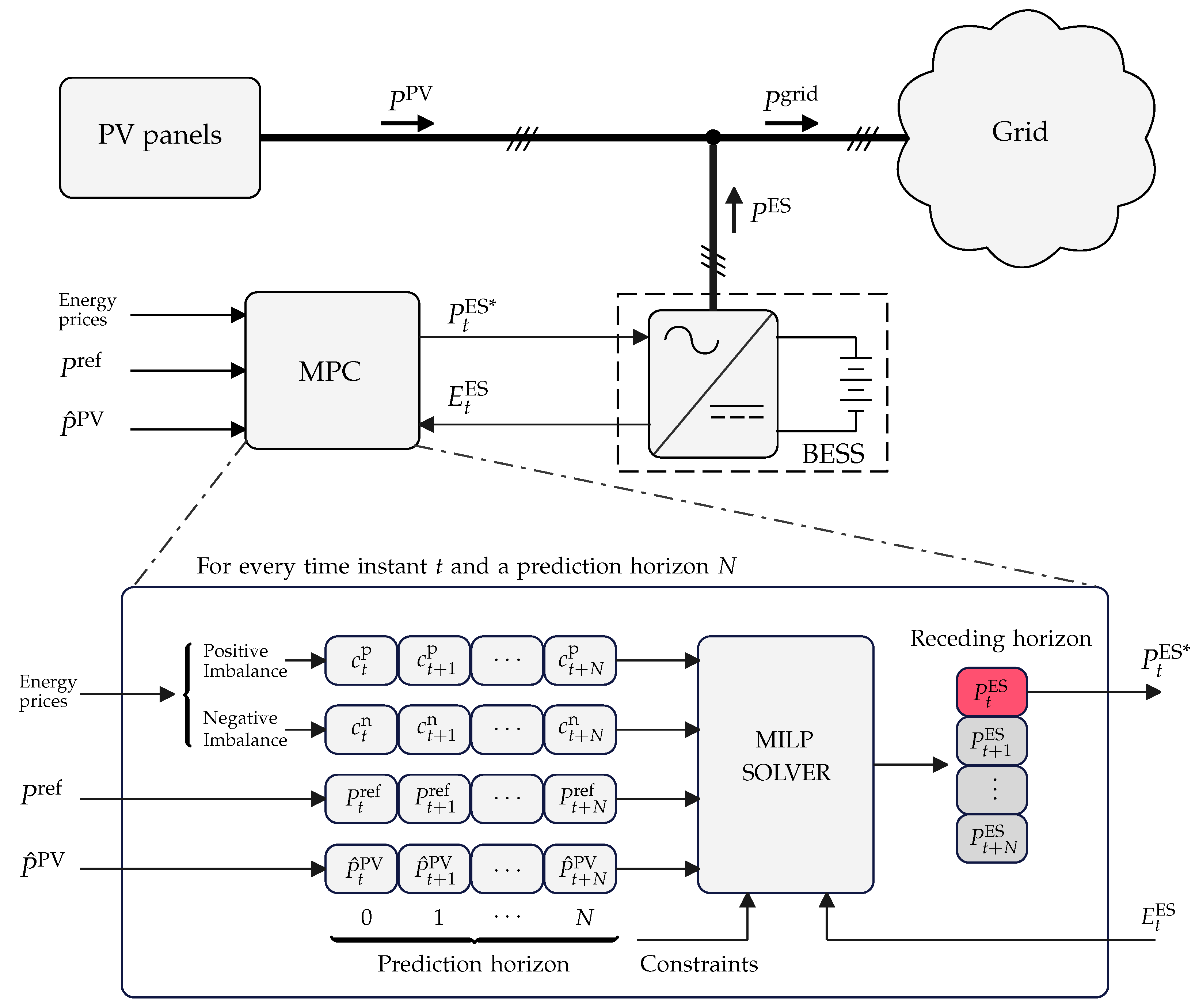
The problem of interest is represented in the diagram of Figure 1. Here, and in the rest of this document, the subscripts t + k , with k = 0 , , N , will symbolize a set of values for a given variable that expands N + 1 samples starting from the current time interval t. In the diagram, P grid is the total power delivered to the grid, corresponding to the sum of the power generated from the PV plant ( P PV ) and the power from the battery system ( P ES ). In the system, a positive value of P ES indicates a power flows from the BESS into the connection node and, therefore, into the grid. Conversely, a negative value of P ES indicates a power flow into the BESS. The value and direction of P ES depend on the decision to either store energy or inject power into the grid ( P ES * ) reached by the MPC algorithm. For simplicity, we consider P ES * = P ES .
The MPC block uses the information of the commitment of constant hourly power to be injected into the grid P ref , the prediction of the energy production from the PV plant P ^ PV , the amount of energy stored in the battery E ES , and energy prices. The variable P ref and the prices are known in advance and E ES can be measured. The prediction P ^ PV can be obtained from statistical information about the behavior of the solar radiation and PV system performance. Particularly, in Europa and Asia, a proper tool is the PhotoVoltaic Geographic Information System (PVGIS) [26]. The energy prices incorporate information about the market structure and the scheduling of settlement periods, which depend on the specific regulations for the given target market.
In the case of the Spanish electricity market, there is a daily market (one day ahead) where an amount of delivered power committed P ref paid at a market price c m is agreed upon, which can be adjusted in an intraday market divided into six sessions of three, four, and five hours to consider variations in the demand forecast and supply contingencies. On the one hand, the intraday market defines the commitment of P ref and c m for the following session. On the other hand, imbalances due to excess or shortage of generation are assigned two different prices around c m that are fixed by the system operator and apply to the difference between the scheduled and actually generated energy. When there is a deviation in the sense of an excess of injected power, the price assigned to this imbalance is c p , with c p c m . On the other hand, when there is a negative difference between the injected power and the committed power, i.e., the producer fails to fulfill his contract, a penalty price c n is applied, with c n c m . To adjust the imbalances, the system operator purchases from generators capable of supplying the missing energy, and the penalty price c n is imposed on the producer who generated the imbalance to cover this cost. The programming of the production market and the price of energy can be obtained in real-time through information provided by the system operator.
As is shown in the zooming part of Figure 1, for every time instant t, the block MPC uses the energy prices, the commitment power, and the prediction of the PV production along the entire prediction horizon, i.e., c t + k p , c t + k n , P t + k ref , and P ^ t + k PV . Combining this information with the amount of energy stored in the battery and a set of constraints over the decision variables, the MPC strategy obtains an optimal control vector by solving a constrained optimization problem. Then, only the first element P t ES of this vector is applied to the system.

2.3. Mathematical Formulation for the Cost Function for the MPC Scheme

To maximize the economic revenue from PV generation, the cost function should account for the following situations:
  • If the PV plant generates more than the committed energy, then the excess energy can be either delivered to the grid or stored in the BESS for future delivery. The energy stored in the BESS can be delivered to the grid in excess during periods when the energy prices are higher or used to attenuate economic penalties when the PV production is lower than the committed.
  • If the PV is anticipated to generate less than the committed energy during some time intervals, then the control algorithm should use the energy stored in the BESS to cover the deficit or shift the failure to moments when the economic penalties are lower.
  • The decision to charge the battery with energy from the PV plant, inject energy from the battery to the grid, or leave the battery idle is taken at every time interval targeting maximization of the economic revenue considering the forecast of energy prices, expected energy production, and state of charge of the battery along the prediction horizon.
Considering the behavior above, authors in [6] specify the following cost function:
max P t + k ES J 1 = c t + N + 1 soc E t + N + 1 ES + k = 0 N α k c t + k T ( P t + k grid P t + k ref ) , s . t .
c t + k = c t + k p if P t + k grid P t + k ref 0 , c t + k n if P t + k grid P t + k ref < 0 ,
P t + k grid = P ^ t + k PV + P t + k ES ,
E t + k + 1 ES = E t + k ES T P t + k ES ,
P min ES P t + k ES P max ES ,
E min ES E t + k ES E max ES ,
where c t + k is the imbalance settlement price that at any given instant adopts a different value depending on the imbalance sign (see Equation (2)); T is the sampling period of the system in which the MPC’s control signal should be available; α 0 , 1 is a weighting parameter, E t + N + 1 ES represents the energy remaining in the BESS after the prediction horizon and c t + N + 1 soc is the price assigned to it. The first term of J 1 sums the expected economic revenues obtained from power delivered to the grid for each interval in the prediction horizon, giving more relevance to the projected economic benefits obtained from time intervals further away from the current time. The second term in the cost function that gives an economic value to the remaining energy stored in the BESS after the prediction horizon. If the parameter c t + N + 1 soc is close to c n , then the control action will favor the accumulation of energy for future sale; conversely, if the value is closer to c p , then the control action will favor the delivery of energy from the BESS to the grid in the current time interval.
The restriction in Equation (3) indicates that the power delivered to the grid corresponds to the sum of the estimated power of photovoltaic panels and the power exchanged with the BESS. Equation (4) models the energy stored in the BESS on the whole prediction horizon. Equation (5) indicates that the power taken from the panels or delivered to the grid from the BESS is limited by the rated power capacity of the converter, and Equation (6) restricts the state of charge of the battery bank to avoid its accelerated degradation or damage. The selection of the sampling time (T) varies depending on the application of interest. The main factors that intervene in the appropriate selection of T depend on the size of the problem and the time constraints. In previous works that apply MPC strategies for controlling similar power generation systems, authors have proposed values of T = 15 min [21,23] and T = 4 min [6] to satisfy the control objectives.
The piece-wise expression for the cost in Equation (2) precludes using standard Linear Programming or Quadratic Programming solvers to find the solution. The authors in [6] identify this as a big limitation to achieving the required solving time of 4 min. Then they propose ad hoc simplifications to represent the cost function in an LP form that can be efficiently solved with standard solvers. Notice that the piece-wise constraints in Equation (2) are common in many applications such as [27,28], where there are variables that can take different values depending on whether a condition is met.

2.4. Representation as an LP Problem

In [6], the authors introduce two different variables to represent the power delivered to the grid depending on its value compared to the committed power:
P t + k grid = P t + k p if P t + k grid P t + k ref , P t + k n if P t + k grid < P t + k ref ,
Using the change of variables and considering the recursive computation of Equation (4), it is possible to rewrite the optimization problem in the following equivalent form [6]:
max P t + k p , P t + k n J 1 * = c t + N + 1 soc E t + N + 1 ES + k = 0 N α k T c t + k p ( P t + k p P t + k ref ) + c t + k n ( P t + k n P t + k ref ) , s . t .
P t + k p + P t + k n P t + k ref = P ^ t + k PV + P t + k ES ,
E t + k + 1 ES = E t + k ES T P t + k ES ,
P min ES P t + k ES P max ES ,
E min ES E t + k ES E max ES ,
P t + k p P t + k ref ,
P t + k n P t + k ref ,
( P t + k p P t + k ref ) ( P t + k n P t + k ref ) = 0 ,
Although the non-linear constraint in Equation (15) still precludes us from directly using traditional LP solvers, the authors in [6] argue that this product constraint is redundant when the other constraints are satisfied and c t + k n c t + k p for all time intervals within the prediction horizon, which is a natural condition in the target scenario. Therefore, it is possible to just omit this constraint, and the resulting optimization problem involves only linear cost function and linear constraints, i.e., an LP problem that can be efficiently solved using traditional tools.
Nevertheless, this solution involves an ad hoc transformation and is not directly applicable for a related problem that includes some other non-linearities such rate-based variable battery efficiency. Additionally, the work in [6] does not show the development with sufficient detail to directly reproduce the reported results. For completeness and, in order to compare our proposal with [6], we provide details in Appendix B to solve the optimization problem in Equation (8). It is noted that this problem cannot be solved directly with an available linear optimization solver, so it is necessary to rewrite it in the standard form of linear programming problems as follows:
max s h T s ,
s . t . Ds d ,
where h summarizes the imbalance costs and the stored energy price over the prediction horizon. The vector s contains the decision variables P t + k p and P t + k n with k = 0 , , N . The vector d and the matrix D define the constraints in Equations (9)–(14). The definitions of h , s , d , and D are given in Appendix B. As can be seen, the problem posed by Equations (16) and (17) has the form of an LP optimization problem, where the upper and lower bound constraints of the decision variables have been rewritten as inequality constraints.

2.5. Implementation of the MPC Schemes and Measurement of Execution Time

To implement and compare the reference LP formulation for the optimization problem described previously and the new MILP formulation introduced in the next section, we use Matlab-Simulink to simulate the system described in Figure 1, including the CPLEX optimization toolbox [29] to solve the optimization problem for each MPC iteration. To estimate the execution time, we use the tic-toc functionality in Matlab to measure the elapsed time between two points of interest in the code. We measure the required time of the solver to get the optimal input vector for 165 MPC iterations. The worst-case value of the elapsed time is reported to show that our proposal is competitive to solve each MPC optimization problem in the required time. All tests were executed on a desktop computer with an Intel Core i7-8700 CPU @ 3.20 GHz processor, 16 GB of RAM, running Windows 11 and MATLAB 2019b.

3. Formulation of the New MPC-MILP Approach

We propose rewriting the problem of the optimal economic management of the storage system in a PV generation plant using an MILP approach. One of the advantages of the MILP approach is that the proposed control strategy can be adapted to the current conditions of the electricity market, as will be discussed later in Section 5.

3.1. Mathematical Formulation Considering an Ideal Battery

In order to solve the problem in (1) using MILP approach, the equality constraints in Equations (3) and (4) were introduced in the cost function J 1 , yielding the following optimization problem:
max P t + k ES J 1 = k = 0 N c t + k T P t + k ES ( P t + k ref P ^ t + k PV ) c t + N + 1 soc T P t + k ES , s . t .
c t + k = α k c t + k p if P t + k ES ( P t + k ref P ^ t + k PV ) 0 , α k c t + k n if P t + k ES ( P t + k ref P ^ t + k PV ) < 0 ,
P min ES P t + k ES P max ES ,
E min ES E t ES T s = 0 k 1 P t + s ES E max ES .
In Appendix C, we explain how to transform an optimization problem involving logical rules into an MILP problem. We consider a binary variable to deal with the condition c t + k that takes different values as P t + k ES is higher or lower than ( P t + k ref P ^ t + k PV ) . The condition P t + k ES ( P t + k ref P ^ t + k PV ) 0 can be associated to a binary variable δ t + k 0 , 1 such that
P t + k ES ( P t + k ref P ^ t + k PV ) 0 δ t + k = 1 .
Since P t + k ES is bounded by P min and P max , the logical statement in Equation (22) can be rewritten as linear constraints. Additionally, introducing a new continuous variable z t + k as follows:
z t + k = P t + k ES ( P t + k ref P ^ t + k PV ) δ t + k ,
which also can be rewritten as linear constraints, then the optimization problem in Equation (18) is equivalent to:
max P t + k ES J 1 + = k = 0 N α k T c t + k p c t + k n z t + k + ( α k c t + k n c t + N + 1 soc ) T P t + k ES , s . t .
P t + k ES P min ( P t + k ref P ^ t + k PV ) ( 1 δ t + k ) + ( P t + k ref P ^ t + k PV ) ,
P t + k ES P max ( P t + k ref P ^ t + k PV ) δ t + k + ( P t + k ref P ^ t + k PV ) ,
z t + k P min ( P t + k ref P ^ t + k PV ) δ t + k ,
z t + k P max ( P t + k ref P ^ t + k PV ) δ t + k ,
z t + k P t + k ES ( P t + k ref P ^ t + k PV ) P min ( P t + k ref P ^ t + k PV ) ( 1 δ t + k ) ,
z t + k P t + k ES ( P t + k ref P ^ t + k PV ) P max ( P t + k ref P ^ t + k PV ) ( 1 δ t + k ) ,
δ t + k 0 , 1 ,
E min ES E t ES T s = 0 k 1 P t + s ES E max ES , k = 1 , , N
where J 1 + stands for an equivalent problem of J 1 . Then, using the definitions in Appendix A, this problem can be rewritten in short form as follows:
max x X f T x ,
s . t . Ax a ,
where f summarizes the imbalance costs and the value of the stored energy over the prediction horizon. The vector x contains the continuous decision variables P t + k ES and z t + k , and the logical decision variable δ t + k over the prediction horizon N. The vector a and the matrix A , contains the constraints in Equations (25)–(32). The set X is the space that contains all possible values of x . The definitions of f , x , a , and A are given in the Appendix D. Note that the change of variable proposed in Equation (22) requires an algorithm that allows the use of binary variables in the formulation, which is not possible with the LP solution proposed in [6]. Therefore, the optimization problem in Equation (33) is solved using standard solvers for MILP.

3.2. Validation Considering an Ideal Battery

To corroborate the functional equivalence between the solution with MPC-LP reported in Section 2 from previous literature and the proposed solution using MPC-MILP, we simulate the same system and conditions reported for the experiments in [6]. Table 1 shows the parameters of the PV+BESS plant and the MPC control parameters.
In this scenario, an ideal battery model with 100 % efficiency is considered. In other words, it is assumed that there are no losses in the charging and discharging processes in the battery, so the energy stored in the battery is equal to the energy available for subsequent discharge.
The data used for the MPC control algorithm explained in Section 2.2 are shown in Figure 2a–c, which correspond to the prices of one simulated day of the Spanish market, the committed power, and the estimated power, respectively. The moment of interest to sell energy in this context is when the committed power has been settled, where the MPC control algorithm acts optimally to generate economic profit or, in the worst case, reduce possible penalties due to the stochastic character of the power coming from the solar panels. As shown in Figure 2c, from 8:00 to 19:00 hours is the period that the estimated power generation from the panels is available. Therefore, it is possible to sell the total power of the plant or accumulate energy in the batteries.
The test scenario considers that the BESS has 25% of its total energy capacity at 8:00 hours. Figure 3a shows how both algorithms decide to completely discharge the batteries, equivalent to supplying all the available energy to the grid. This makes sense since both control algorithms have the same prior knowledge to act optimally to increase profits. In this case, the power generated by the PV-BESS system is greater than the committed power, as shown in Figure 3b, which increases the economic revenue according to the imbalance price. It can also be seen that throughout the operation of the system, the total power supplied to the grid is bigger than the committed power, which verifies that both algorithms avoid penalties. Starting at 11:00 hours, the BESS stores energy from the solar panels as indicated by negative values of P t ES in Figure 3c. The simulation results also show in Figure 3d that the heuristic solution employing MPC-LP proposed in [6] is valid and equivalent to the formulation MPC-MILP proposed in this work when considering an ideal battery. As can be seen, the results obtained with the proposed MPC-MILP formulation are validated by simulation results, offering the same performance as the strategy available in the literature.
Additionally, the measurements of the execution time for both MPC-LP and MPC-MILP, in the worst case, were about 18 and 46 milliseconds, respectively. As we explained above, the time required for the control algorithm to make the optimal decision in the PV-BESS application is T = 4 min. It is noted that although the time required by the algorithms is not deterministic, the control signal is found quickly enough to actuate over the system. This fact shows that the MILP approach is not computationally prohibitive for real-time operation as the initial assumption in [6].
So far, it has been shown how to perform the MPC control considering an idealized battery model. The described problem has not considered the losses of the charging and discharging of the batteries. Neglecting these parameters can result in poor decision-making by the control algorithm. Consequently, in Figure 3a, a high amount of charging and discharging can be seen. Next, an alternative solution considering a model for the efficiency of the charging and discharging of the battery is proposed.

3.3. Formulation Considering BESS with Rate-Based Variable Efficiency

In this section, the same problem of interest as [6] that has been already discussed in Section 2.3 is considered, but introducing the charge and discharge efficiency of the battery. In this work, it is considered that the BESS is charged with constant rate efficiency η c and discharged with 1 / η d , and it is not directly solvable using [6]. We note that both of these efficiencies are positive quantities, and smaller than one, as expected ( 0 < η c 1 and 0 < η d 1 ) . However, as the objective function values the stored energy in the battery, the definition of efficiency must correspond to the natural definition for the charging efficiency, regardless of the actual operational condition. This leads to an efficiency definition as Equation (37) where η c 1 for charging ( P t ES < 0 ) and 1 / η d 1 for discharging ( P t ES 0 ) . Then, the problem to solve is the following:
max P t + k ES J 2 = k = 0 N c t + k T P t + k ES ( P t + k ref P ^ t + k PV ) c t + N + 1 soc T η t + k P t + k ES , s . t .
c t + k = α k c t + k p if P t + k ES ( P t + k ref P ^ t + k PV ) 0 , α k c t + k n if P t + k ES ( P t + k ref P ^ t + k PV ) < 0 ,
η t + k = 1 / η d if P t + k ES 0 , η c if P t + k ES < 0 ,
P min ES P t + k ES P max ES ,
E min ES E t ES T s = 0 k 1 η t + k P t + s ES E max ES .
To solve this problem, an approach similar to Section 3 is used. Consider a binary value to deal with the logical condition on η t + k :
P t + k ES 0 β t + k = 1 .
Additionally, a continuous auxiliary variable w t + k is introduced so that w t + k = P t + k ES β t + k . Then, following Appendix C the optimization problem in Equation (35) can be rewritten as follows:
max P t + k ES J 2 + = k = 0 N α k T c t + k p c t + k n z t + k + T ( α k c t + k n c t + N + 1 soc η c ) P t + k ES c t + N + 1 soc T ( η d η c ) w t + k , s . t .
P t + k ES P min ( P t + k ref P ^ t + k PV ) ( 1 δ t + k ) + ( P t + k ref P ^ t + k PV ) ,
P t + k ES P max ( P t + k ref P ^ t + k PV ) δ t + k + ( P t + k ref P ^ t + k PV ) ,
z t + k P min ( P t + k ref P ^ t + k PV ) δ t + k ,
z t + k P max ( P t + k ref P ^ t + k PV ) δ t + k ,
z t + k P t + k ES ( P t + k ref P ^ t + k PV ) P min ( P t + k ref P ^ t + k PV ) ( 1 δ t + k ) ,
z t + k P t + k ES ( P t + k ref P ^ t + k PV ) P max ( P t + k ref P ^ t + k PV ) ( 1 δ t + k ) ,
P t + k ES P min ( 1 β t + k ) ,
P t + k ES P max β t + k ,
w t + k P min β t + k ,
w t + k P max β t + k ,
w t + k P t + k ES P min ( 1 β t + k ) ,
w t + k P t + k ES P max ( 1 β t + k ) ,
δ t + k 0 , 1 ,
β t + k 0 , 1 ,
( δ t + k β t + k ) ( P t + k ref P ^ t + k PV ) 0 ,
E min ES E t ES T s = 0 k 1 η t + k P t + s ES E max ES , k = 1 , , N ,
where J 2 + stands for an equivalent problem of J 2 . Then, using the definitions in Appendix A, this MILP problem can be rewritten in short form as follows:
max y Y g T y ,
s . t . B y b ,
where g summarizes the imbalance costs and the value of the stored energy over the prediction horizon. The vector y contains the continuous decision variables P t + k ES , z t + k and w t + k , and the logical decision variables δ t + k and β t + k over the prediction horizon N. The vector b and the matrix B , contains the constraints in Equations (42)–(57). The set Y is the space that contains all possible values of y . The definitions of g , y , b , and B are given in the Appendix E.
Next, the results of the simulation of the proposed formulation applied to a BESS with non-ideal charge and discharge efficiency are shown and compared with the results achieved when solved with the technique presented in Section 2.4, i.e., when assuming ideal efficiency in the control. In other words, the objective is to identify the economic benefit of using MPC-MILP in PV-BESS, considering a rate-based variable efficiency model for the battery, and compare it to the solution obtained with the MPC-LP strategy reported in the literature.

4. Results

The response of the MPC-LP, as described in Section 2.4, and the proposed MPC-MILP control algorithms, when applied to a system model with non-ideal charge and discharge efficiency, are shown. The initial conditions are the same as in the previous section. Figure 4 shows the comparison of the results obtained using the MPC-LP and MPC-MILP control algorithms. As can be seen, the system’s dynamic performance with the MPC-MILP control algorithm and a BESS model with a rate-based variable efficiency is notably better. Figure 4a shows how the performance of the MPC-MILP algorithm does not completely discharge the battery, unlike MPC-LP. Although both algorithms satisfy the output power needed to avoid a penalty, i.e., P grid P ref , the power transients are less aggressive using the strategy MPC-MILP, as shown in Figure 4b. This is a direct consequence of making decisions about the charging and discharging cycles in the batteries, as shown in Figure 4c. It is also noted that reducing charge and discharge cycles contributes to extending the BESS’s health. The improvements obtained in the simulation results are understandable from a physical point of view. When considering a simplified battery model, the algorithm described in Section 2.4 estimates the charging and discharging processes with less precision because it does not consider the losses associated with the power exchanged with the BESS. This fact translates into a poor decision to store energy in the BESS or sell it to the power grid. While the MPC-LP algorithm acts aggressively, the MPC-MILP algorithm performs better in making decisions to supply power, charge the batteries or disconnect them from the system. Figure 4d shows how the proposed control algorithm obtains a bigger J 2 over time compared with the MILP-LP, which is the main control objective, i.e., it makes the PV plant’s market participation more profitable. The computation of the cost function J 2 using the optimal control signal of each time instant shows that the increment in the economic revenues obtained using our proposal is close to 21% with respect to the MPC-LP approach.
Furthermore, the execution time of the model that considers the rate-based variable efficiency increases with respect to the highly efficient MPC-LP method proposed in [6]. However, the solution of the MPC-MILP algorithm in the worst case was found in 55 milliseconds, which is still small enough for T = 4 min. Additionally, the measurements for both MPC-LP and MPC-MILP, in the worst case, were about 18 and 46 milliseconds, respectively.

Influence of the Solar Radiation Estimation in the Control Scheme

In this section, a study of the influence of solar estimation on the performance of the control algorithm is carried out. As mentioned above, the database provided by PVGIS is used in this work. However, the estimated data could differ from the actual radiation due to the presence of meteorological phenomena, causing the stochastic behavior of this energy source. Estimated solar radiation data will become more accurate as parameter estimation techniques evolve. It should be considered that an inaccurate P ^ t PV estimation model could lead to penalties in the market under the aforementioned conditions. An experiment is then carried out to assess how much the difference between the estimated P ^ t PV power used in the control algorithm and the actual P ^ t PV power can affect. Figure 5a shows an example of the difference in solar radiation on a slightly cloudy day.
Under these conditions, the actual P ^ t PV is less than the model used in the algorithm. In this test, the approach described in the Section 2.4 and the one proposed in Section 3.3 are compared. The Figure 5b shows the objective function for both control algorithms. As can be seen, the MPC-MILP approach proposed in this work continues to generate higher economic returns compared to the MPC-LP approach.

5. Discussion

The use of the MPC strategy has increased in recent years for electric power generation due to its advantages. In particular, it allows optimal decision-making considering the physical and operational constraints of the system. The proposal incorporated can implement more realistic models of the storage system, including its efficiency, leading to better performance of the control loop than a previous method found in the literature, translating into higher earnings for the market participant.
This article provides a detailed methodology for the mathematical formulation of the optimization problem using the paradigm of Mixed Integer Linear Programming. Additionally, some measurements of the computational burden of this method are provided, showing that although higher than the alternative method found in [6], it is sufficiently low for the problem of interest, given the computational capability of modern desktop computers. Future work may consider integrating other energy sources, whether renewable or non-renewable, and applying the control algorithm to plants integrating different generation technologies to minimize energy production costs. Further, the proposed methodology can be adapted to different problems with similar characteristics.
This is very important, as rules in regulated markets are different from country to country and may change with new regulations. For example, the operating procedure through the provisions of P.O.-14.1 in the Spanish market has undergone recent modifications, where now there are four situations in which participating agents can incur in the market. However, we emphasize that the proposed control scheme can be directly applied to the new circumstances because it can adequately consider the value of c t + k in the constraints of the optimization problem for each situation.

6. Conclusions

This study investigates how to obtain economic benefits by participating in the Spanish electricity market. This work presents a new control strategy that incorporates the charging and discharging efficiency of the BESS model in PV plants with storage. The proposed strategy maximizes the economic benefit of a given power scheduling in electricity market participation by optimizing the use of the battery storage system. The proposal is validated by simulation results and compared with important previous works that do not consider the battery efficiency model. Three simulation examples show that the MPC-MILP algorithm can maintain the power above or equal to the committed power thanks to the integration of the BESS. The simulation results also show how the rate-based variable efficiency battery model can further improve the economic benefit using an MPC-MILP approach. It is also shown that with modern desktop computers, the proposed control is feasible within a sampling period of T = 4 min sufficient for the intended application. Consequently, we believe that the proposed control methodology will allow an increased number of agents to be more competitive in the market, eventually potentially reducing the final cost to consumers and to society.

Author Contributions

Conceptualization, A.L.C., R.L.A., C.S. and J.C.A.; methodology, A.L.C., R.L.A., C.S. and J.C.A.; software, A.L.C.; validation, J.R. and G.C.; formal analysis, A.L.C., R.L.A., J.R., G.C., C.S. and J.C.A.; investigation, A.L.C., R.L.A., G.C., C.S. and J.C.A.; resources, G.C., C.S. and J.C.A.; writing—original draft preparation, A.L.C., R.L.A., J.R., G.C., C.S. and J.C.A.; writing—review and editing, A.L.C., R.L.A., J.R., G.C., C.S. and J.C.A.; visualization, G.C.; supervision, G.C., C.S. and J.C.A. All authors have read and agreed to the published version of the manuscript.

Funding

This work was supported in part by the Chilean National Agency for Research and Development (ANID) Scholarship Program/doctorado nacional/2020-21202410 and 2021-21211446, in part by the PIIC program of DGP at Universidad Técnica Federico Santa María No 047/2021 and 048/2018, and in part by the grants ANID-Fondecyt 1211630 and 1211676, ANID-Basal Project FB0008 (AC3E) and ANID-PIA/Apoyo AFB180002 (CCTVal).

Institutional Review Board Statement

Not applicable.

Informed Consent Statement

Not applicable.

Data Availability Statement

No new data were created or analyzed in this study. Data sharing is not applicable to this article.

Conflicts of Interest

The authors declare no conflict of interest.

Abbreviations

The following abbreviations are used in this manuscript:
MPCModel Predictive Control
MILPMixed-Integer Linear Programming
PVPhotovoltaic
ACAlternating Current
DCDirect Current
BESSBattery Energy Storage System
SoCState of Charge
LPLinearProgramming
QPQuadratic Programming
PSDPower Spectral Density
PVGISPhotoVoltaic Geographic Information System
CPLEXIBM ILOG CPLEX Optimization Studio

Appendix A

Vector and matrices for the problem in Equation (1) considering a prediction horizon N:
α = 1 α 1 α N , c n = c t n c t + 1 n c t + N n , c p = c t p c t + 1 p c t + N p , c soc = c t + N + 1 soc c t + N + 1 soc c t + N + 1 soc ,
P min = P min ES P min ES P min ES , P max = P max ES P max ES P max ES , P ref = P t ref P t + 1 ref P t + N ref , P ^ PV = P ^ t PV P ^ t + 1 PV P ^ t + N PV ,
E min = 1 T E t ES E max ES E t ES E max ES E t ES E max ES , E max = 1 T E t ES E min ES E t ES E min ES E t ES E min ES , F = 1 0 0 1 1 0 1 1 1 ,
where α , c n , c p , c soc , P min , P max , P ref , E min , P ^ PV , E max R N + 1 and F R N + 1 × N + 1 . I R N + 1 × N + 1 is the identity matrix. Additionally, 0 represents the zero vector or matrix, and its dimensions should be inferred from the context, i.e., 0 is a vector R N + 1 or is a matrix R N + 1 × N + 1 .

Appendix B. Vectors and Matrices for the Solution in [6]

In this section, the following vectors and matrices are introduced to solve the LP problem given in Equations (16)–(17). Considering Equation (16), the vector h is given by
h = h 1 h 2 , h 1 = α c p c soc , h 2 = α c n c soc ,
where ⊙ is the element-wise product operator, α , c p , c n and c soc are defined in the Appendix A. The vector s in Equation (16) contains the decision vectors P p and P n that are given by
s = P p P n , P p = P t p P t + 1 p P t + N p , P n = P t n P t + 1 n P t + N n ,
where P p , P n R N + 1 . On the other hand, considering Equation (17), the matrix inequality D and the vector d are given by
D = I I I I F F F F I 0 0 I , d = ( P min + P ref + P ^ PV ) P max + P ref + P ^ PV ( E min + F ( P ref + P ^ PV ) ) E max + F ( P ref + P ^ PV ) P ref P ref ,
where all vectors and matrices in d and D are defined in the Appendix A.

Appendix C. Two Equivalent Optimization Problems

Consider the problem to maximize a function upper and lower bounded by M and m, respectively, and subject to logical rules as follows:
max g ( x ) = ρ f ( x ) , s . t .
m f ( x ) M ,
ρ = a if f ( x ) 0 , b if f ( x ) < 0 ,
where f ( x ) = A x + c and m 0 . In this appendix, we show that the optimization in Equations (A7)–(A9) can be rewritten as an MILP. Following [30,31], the condition f ( x ) 0 can be associated to a binary variable δ { 0 , 1 } such that:
m f ( x ) M , f ( x ) 0 , δ = 1 ,
then, Equation (A10) can be expressed by the following inequalities:
f ( x ) m ( 1 δ ) ,
f ( x ) + ϵ ( M + ϵ ) δ ,
where ϵ is a small positive scalar that represents a tolerance typically chosen as the machine precision. Then, the function g ( x ) can be rewritten as:
g ( x ) = ( a b ) δ f ( x ) + b f ( x ) .
In fact, δ = 1 g ( x ) = a f ( x ) and δ = 0 g ( x ) = b f ( x ) , which is equivalent to Equations (A7)–(A9). In order to deal with the product of a continuous and a logical variable δ f ( x ) in Equation (A13), a new variable z = δ f ( x ) is introduced (see, e.g., [32]). This new variable can be rewritten as follows:
z M δ ,
z m δ ,
z f ( x ) m ( 1 δ ) ,
z f ( x ) M ( 1 δ ) .
In fact, δ = 1 ( m z M , z = f ( x ) ) and δ = 0 ( z = 0 , m f ( x ) M ) . Finally, the problem in Equations (A7)–(A9) can be written as
max g ( x ) = ( a b ) z + b f ( x ) , s . t .
z M δ ,
z m δ ,
z f ( x ) m ( 1 δ ) ,
z f ( x ) M ( 1 δ ) ,
f ( x ) m ( 1 δ ) ,
f ( x ) + ϵ ( M + ϵ ) δ .
This optimization problem is an MILP.

Appendix D. Vectors and Matrices for the MPC-MILP Solution

In this section, the following vectors and matrices are introduced to solve the MPC-MILP problem given in Equations (33) and (34). Considering Equation (33), the vector f is given by
f = f 1 f 2 0 , f 1 = α c n c soc , f 2 = α ( c p c n ) ,
where ⊙ is the element-wise product operator, α , c p , c n and c soc are defined in the Appendix A. The vector x in Equation (33) contains the continuous vectors P ES and z , and the logical vector δ that are given by
x = P ES z δ , P ES = P t ES P t + 1 ES P t + N ES , z = z t z t + 1 z t + N , δ = δ t δ t + 1 δ t + N .
where P ES , z , δ R N + 1 . Notice that some components in the variable x are reals and other are integers, which defines the set X in Equation (33). Considering Equation (34), the matrix inequality A and the vector a are given by
A = I 0 diag P min R I 0 diag P max R 0 I + diag P min R 0 I diag P max R I I diag P min R I I + diag P max R F 0 0 F 0 0 , a = P min R 0 0 P min P max E max E min .
All vectors and matrices in a and A are defined in the Appendix A, except R = P ref P ^ PV .

Appendix E. Vectors and Matrices for the MPC-MILP Solution with Rate-Based

In this section, the following vectors and matrices are introduced to solve the MPC-MILP problem given in Equations (58) and (59). Considering Equation (58), the vector g is given by
g = g 1 g 2 0 g 3 0 , g 1 = α c n c soc η c , g 2 = α ( c p c n ) , g 3 = c soc ( η c η d ) , η c = η c η c η c , η d = 1 / η d 1 / η d 1 / η d ,
where ⊙ is the element-wise product operator, α , c p , c n and c soc are defined in the Appendix A, and η c , η d R N + 1 . The vector y in Equation (58) contains the continuous vectors P ES , z , w and the logical vectors δ and β that are given by
y = P ES z δ w β , w = w t w t + 1 w t + N , β = β t β t + 1 β t + N ,
with P ES , z , and δ given in Equation (A26) and w , β R N + 1 . Notice that some components in the variable y are reals and other are integers, which defines the set Y in Equation (58). On the other hand, consider Equation (59), then the matrix inequality B and the vector b are given by
B = I 0 diag P min R 0 0 I 0 diag P max R 0 0 0 I + diag P min R 0 0 0 I diag P max R 0 0 I I diag P min R 0 0 I I + diag P max R 0 0 I 0 0 0 diag P min I 0 0 0 diag P max 0 0 0 I + diag P min 0 0 0 I diag P max I 0 0 I diag P min I 0 0 I + diag P max V 1 0 0 V 2 0 V 1 0 0 V 2 0 0 0 diag R 0 diag R , b = P min R 0 0 P min P max P min 0 0 0 P min P max E max E min 0 ,
where the matrices V 1 and V 2 can be computed following: V 1 = F η c and V 2 = F ( η d η c ) and the remainder terms in b and B are defined in the Appendix A, except R = P ref P ^ PV . Notice that, if η d = η c = 1 , the optimization problem becomes the original problem in Section 2.4.

References

  1. Cubukcu, M.; Gumus, H. Performance analysis of a grid-connected photovoltaic plant in eastern Turkey. Sustain. Energy Technol. Assess. 2020, 39, 100724. [Google Scholar] [CrossRef]
  2. Fuentealba, E.; Ferrada, P.; Araya, F.; Marzo, A.; Parrado, C.; Portillo, C. Photovoltaic performance and LCoE comparison at the coastal zone of the Atacama Desert, Chile. Energy Convers. Manag. 2015, 95, 181–186. [Google Scholar] [CrossRef]
  3. Rebolledo, F.; Mendoza-Araya, P.; Carvajal, G.; Ramírez, R. Performance evaluation of different solar modules and mounting structures on an on-grid photovoltaic system in south-central Chile. Energy Sustain. Dev. 2022, 68, 65–75. [Google Scholar] [CrossRef]
  4. Mohammadi, K.; Naderi, M.; Saghafifar, M. Economic feasibility of developing grid-connected photovoltaic plants in the southern coast of Iran. Energy 2018, 156, 17–31. [Google Scholar] [CrossRef]
  5. Khan, B.; Mahela, O.P.; Alhelou, H.H.; Padmanaban, S. Deregulated Electricity Market: The Smart Grid Perspective; Apple Academic Press: Palm Bay, FL, USA, 2022. [Google Scholar]
  6. Perez, E.; Beltran, H.; Aparicio, N.; Rodríguez, P. Predictive Power Control for PV Plants With Energy Storage. IEEE Trans. Sustain. Energy 2012, 4, 482–490. [Google Scholar] [CrossRef]
  7. Ando, R.; Ishii, H.; Hayashi, Y.; Zhu, G. A Planned Power Generation for Battery-Assisted Photovoltaic System Using Short-Term Forecast. IEEE Access 2021, 9, 125238–125246. [Google Scholar] [CrossRef]
  8. ESIOS. Red eléctrica de España. Sistema de Información del Operador del Sistema. 2022. Available online: https://www.esios.ree.es (accessed on 30 August 2022).
  9. Ullah, Z.; Arshad; Hassanin, H. Modeling, Optimization, and Analysis of a Virtual Power Plant Demand Response Mechanism for the Internal Electricity Market Considering the Uncertainty of Renewable Energy Sources. Energies 2022, 15, 5296. [Google Scholar] [CrossRef]
  10. DiOrio, N.; Denholm, P.; Hobbs, W.B. A model for evaluating the configuration and dispatch of PV plus battery power plants. Appl. Energy 2020, 262, 114465. [Google Scholar] [CrossRef]
  11. Bullich-Massagué, E.; Cifuentes-García, F.; Glenny-Crende, I.; Cheah-Mañé, M.; Aragüés-Peñalba, M.; Díaz-González, F.; Gomis-Bellmunt, O. A review of energy storage technologies for large scale photovoltaic power plants. Appl. Energy 2020, 274, 115213. [Google Scholar] [CrossRef]
  12. Arsalis, A.; Papanastasiou, P.; Georghiou, G.E. A comparative review of lithium-ion battery and regenerative hydrogen fuel cell technologies for integration with photovoltaic applications. Renew. Energy 2022, 191, 943–960. [Google Scholar] [CrossRef]
  13. Ai, X.; Li, J.; Fang, J.; Yao, W.; Xie, H.; Cai, R.; Wen, J. Multi-time-scale coordinated ramp-rate control for photovoltaic plants and battery energy storage. IET Renew. Power Gener. 2018, 12, 1390–1397. [Google Scholar] [CrossRef]
  14. Hu, Y.; Armada, M.; Jesús Sánchez, M. Potential utilization of battery energy storage systems (BESS) in the major European electricity markets. Appl. Energy 2022, 322, 119512. [Google Scholar] [CrossRef]
  15. Souza, L.; Rotella Junior, P.; Aquila, G.; Maheri, A. Multiobjective optimization of hybrid wind-photovoltaic plants with battery energy storage system: Current situation and possible regulatory changes. J. Energy Storage 2022, 51, 104467. [Google Scholar]
  16. Yang, Y.; Bremner, S.; Menictas, C.; Kay, M. A Mixed Receding Horizon Control Strategy for Battery Energy Storage System Scheduling in a Hybrid PV and Wind Power Plant with Different Forecast Techniques. Energies 2019, 12, 2326. [Google Scholar] [CrossRef]
  17. Sánchez de la Nieta, A.A.; Paterakis, N.G.; Gibescu, M. Participation of photovoltaic power producers in short-term electricity markets based on rescheduling and risk-hedging mapping. Appl. Energy 2020, 266, 114741. [Google Scholar] [CrossRef]
  18. Kim, H.; Kwon, W.; Kim, S.; Lee, D. MPC-Based Optimal Operation for a PV Farm With Dual ESSs Using Spectral Density Analysis of Market Signals. IEEE Access 2020, 8, 215457–215466. [Google Scholar] [CrossRef]
  19. Borrelli, F.; Bemporad, A.; Morari, M. Predictive Control for Linear and Hybrid Systems; Cambridge University Press: Cambridge, UK, 2017. [Google Scholar]
  20. Rawlings, J.B.; Mayne, D.Q.; Diehl, M. Model Predictive Control: Theory, Computation, and Design; Nob Hill Publishing: Madison, WI, USA, 2017; Volume 2. [Google Scholar]
  21. Parisio, A.; Rikos, E.; Glielmo, L. A Model Predictive Control Approach to Microgrid Operation Optimization. IEEE Trans. Control Syst. Technol. 2014, 22, 1813–1827. [Google Scholar] [CrossRef]
  22. Kim, R.; Glick, M.B.; Olson, K.R.; Kim, Y. MILP-PSO combined optimization algorithm for an islanded microgrid scheduling with detailed battery ESS efficiency model and policy considerations. Energies 2020, 13, 1898. [Google Scholar] [CrossRef]
  23. Delfino, F.; Ferro, G.; Minciardi, R.; Robba, M.; Rossi, M.; Rossi, M. Identification and optimal control of an electrical storage system for microgrids with renewables. Sustain. Energy Grids Netw. 2019, 17, 100183. [Google Scholar] [CrossRef]
  24. Sigalo, M.B.; Pillai, A.C.; Das, S.; Abusara, M. An Energy Management System for the Control of Battery Storage in a Grid-Connected Microgrid Using Mixed Integer Linear Programming. Energies 2021, 14, 6212. [Google Scholar] [CrossRef]
  25. Achiluzzi, E.; Kobikrishna, K.; Sivabalan, A.; Sabillon, C.; Venkatesh, B. Optimal Asset Planning for Prosumers Considering Energy Storage and Photovoltaic (PV) Units: A Stochastic Approach. Energies 2020, 13, 1813. [Google Scholar] [CrossRef] [Green Version]
  26. PVGIS. Photovoltaic Geographic Information System. 2022. Available online: https://re.jrc.ec.europa.eu (accessed on 30 August 2022).
  27. Foroozandeh, Z.; Ramos, S.; Soares, J.; Lezama, F.; Vale, Z.; Gomes, A.; L. Joench, R. A Mixed Binary Linear Programming Model for Optimal Energy Management of Smart Buildings. Energies 2020, 13, 1719. [Google Scholar] [CrossRef]
  28. Tobajas, J.; Garcia-Torres, F.; Roncero-Sánchez, P.; Vázquez, J.; Bellatreche, L.; Nieto, E. Resilience-oriented schedule of microgrids with hybrid energy storage system using model predictive control. Appl. Energy 2022, 306, 118092. [Google Scholar] [CrossRef]
  29. CPLEX. IBM ILOG CPLEX Optimization Studio. 2022. Available online: https://www.ibm.com/cl-es/products/ilog-cplex-optimization-studio (accessed on 30 August 2022).
  30. Williams, H.P. Model Building in Mathematical Programming; John Wiley & Sons: Hoboken, NJ, USA, 2013. [Google Scholar]
  31. Bemporad, A.; Morari, M. Control of systems integrating logic, dynamics, and constraints. Automatica 1999, 35, 407–427. [Google Scholar] [CrossRef]
  32. Glover, F. Improved Linear Integer Programming Formulations of Nonlinear Integer Problems. Manag. Sci. 1975, 22, 455–460. [Google Scholar] [CrossRef] [Green Version]
Figure 1. Model predictive control scheme.
Energies 15 06427 g001
Figure 2. (a) Synthetic energy prices resembling the ones reported in [6]; (b) committed power per hour; and (c) power production of photovoltaic panels considering ideal solar radiation.
Energies 15 06427 g002
Figure 3. (a) Exchange power with the BESS; (b) cost of the optimization algorithm; (c) energy stored in batteries; and (d) power injected into the grid.
Energies 15 06427 g003
Figure 4. (a) Exchange power with the BESS; (b) cost of the optimization algorithm; (c) energy stored in batteries; and (d) power injected into the grid.
Energies 15 06427 g004
Figure 5. (a) Difference between the estimated power and the real power for a slightly cloudy day (b) Cost of MPC-LP and MPC-MILP algorithms.
Energies 15 06427 g005
Table 1. PV+BESS plant and MPC control parameters.
NT c p c n λ k
604 minas in Figure 2as in Figure 2 0 . 999 k
c t + N + 1 soc P min ES P max ES E min ES E max ES
c n 500 kW500 kW0 0.8 MWh
Publisher’s Note: MDPI stays neutral with regard to jurisdictional claims in published maps and institutional affiliations.

