Article

Applicability of Wake Models to Predictions of Turbine-Induced Velocity Deficit and Wind Farm Power Generation

1
School of Civil and Environmental Engineering, Harbin Institute of Technology, Shenzhen 518055, China
2
Shenzhen Key Laboratory of Intelligent Structure System in Civil Engineering, Harbin Institute of Technology, Shenzhen 518055, China
3
Guangdong-Hong Kong-Macao Joint Laboratory for Data-Driven Fluid Mechanics and Engineering Applications, Harbin Institute of Technology, Shenzhen 518055, China
*
Author to whom correspondence should be addressed.
Energies 2022, 15(19), 7431; https://doi.org/10.3390/en15197431
Submission received: 30 July 2022 / Revised: 2 September 2022 / Accepted: 4 October 2022 / Published: 10 October 2022

Abstract

:
Turbine-induced velocity deficit is the main reason to reduce wind farm power generation and increase the fatigue loadings. It is meaningful to investigate turbine-induced wake structures by a simple and accurate method. In this study, a series of single turbine wake models are proposed by combining different spanwise distributions and wake boundary expansion models. It is found that several combined wake models with high hit rates are more accurate and universal. Subsequently, the wake models for multiple wind turbines are also investigated by considering the combined wake models for single turbine and proper superposition approaches. Several excellent plans are provided where the velocity, turbulence intensity, and wind power generation for multiple wind turbines can be accurately evaluated. Finally, effects of thrust coefficient and ambient turbulence intensity are studied. In summary, the combined wake models for both single and multiple wind turbines are proposed and validated, enhancing the precision of wind farm layout optimization will be helped by using these wake models.

1. Introduction

Wind energy is considered as one of most clean renewable resources and the exploitation of wind power can help us to solve the energy and environment crises. In 2021, the wind turbine capacity added 93.6 GW all over the world, and the global cumulative capacity reached 837 GW. However, it has been pointed out by GWEC that four times as much will be needed annually by 2030 to achieve net-zero emission [1]. Therefore, it is necessary to increase the global wind energy investigation and improve the wind power exploitation efficiency.
Theoretical or empirical wake models are widely used to carry out the wind farm layout optimization (WFLO) due to their simplicity and effectiveness. Therefore, an accurate wake model is the premise of the wind farm layout optimization. Jensen [2] firstly proposed an analytical wake model using the top-hat distribution and mass conservation, and this is widely used to conduct the WFLO. Frandsen et al. [3] also proposed an analytical wake model considering both mass and momentum conservation. Subsequently, Gaussian-based wake models were proposed [4,5] to overcome the discrepancy between top-hat distribution and the measured velocity deficit. Cosine-shaped wake models have also been proposed by Tian et al. [6] and Zhang et al. [7]. It is believed that the Gaussian-based or cosine-shaped wake models are more advanced, and they are consistent with the boundary layer theory. In addition, the 3D wake models [8,9], the full wake models [10,11], and the wake model for offshore wind turbine [12], have also been proposed. All these wake models have been validated by specific experiments or simulations, and wake model comparisons have also been carried out. However, a comprehensive comparison of these wake models with field tests, wind tunnel tests, and numerical simulations has not been carried out and the applicability of these wake models has not been discussed.
There are three main parts of the analytical wake model: the spanwise function, the streamwise function, and the wake boundary expansion model. In general, it is assumed that the spanwise function is distributed as the top-hat, Gaussian, or cosine shape, and the streamwise function can be derived by the spanwise function, the mass and momentum conservation. As for the wake boundary expansion, these are predicted by the empirical models and validated by measured data. The linear wake boundary expansion model with a constant expansion rate is the simplest one [2]. A non-linear model to describe the wake boundary expansion is adopted by Frandsen et al. [3]. To consider the effects of thrust coefficient and ambient turbulence intensity, it is assumed that the expansion rate and the intercept are related to these two parameters by Ishihara and Qian [5]. Furthermore, a non-linear wake boundary expansion model in which the wake radius is influenced with the added turbulence intensity is used [6,7,13]. Researchers have proposed the spanwise distribution, the streamwise function, and the wake boundary expansion model simultaneously, as shown in Table 1, however, the combined wake models (by considering different spanwise distributions, streamwise functions, and wake boundary expansion models) have not been systematically studied.
To calculate the velocity distribution and power generation in the wind farm, the wake velocity needs to be added together properly. A series of empirical superposition approaches for multiple wind turbines have been proposed, including the ambient-based linear superposition approach [14], the rotor-based linear superposition approach [15], the ambient-based root sum square superposition approach [16], the rotor-based root sum square superposition approach [17], the geometric superposition approach [18], and the energy conservation superposition approach [19]. Qian and Ishihara [20] compared the first four superposition approaches and found that the rotor-based linear superposition approach is more suitable for the IQ wake model. Yang et al. [13] and Tian et al. [21] noted that prediction results obtained by the root sum square superposition approach show excellent agreement with numerical simulations. Kirchner-Bossi and Porté-Agel [22] found that the combination of the rotor-based linear superposition approach and the BP wake model is an effective and accurate way to evaluate the wind power generation. The accurate prediction of wind velocity and wind power generation for multiple wind turbines depends on both the single wind turbine wake model and the superposition approach. Therefore, it is necessary to find the suitable superposition approach for a specific single wind turbine wake model.
In this study, the applicability of wake models to predict of turbine-induced velocity deficit and power generation is investigated. Theoretical wake models for single and multiple wind turbines including spanwise and streamwise distributions for velocity deficit, wake boundary expansion, added turbulence intensity, superposition approaches, and the Horn Rev 1 wind farm are introduced in Section 2 and Section 3, respectively. The combined wake models for both single and multiple wind turbines are proposed and validations are also carried out, and effects of thrust coefficient and ambient turbulence intensity on the wind power generation are studied in Section 4. Section 5 summarizes the conclusions.

2. Wake Models for the Single Wind Turbine

A series of analytical and empirical wake models for prediction of the velocity deficit, wake boundary expansion, and added turbulence intensity are introduced in Section 2.1, Section 2.2 and Section 2.3.

2.1. Spanwise and Streamwise Distributions

The mass and momentum conservations of a control volume around a wind turbine can be expressed as:
A 0 ρ U 0 d A = A W ρ U W d A
A 0 ρ U 0 2 d A A W ρ U W 2 d A = 1 2 ρ C T A 0 U 0 2
where U 0 , A 0 represent the inflow wind speed at hub height and the rotor area. U W , A W refer to the wind velocity and the cross-sectional area influenced by wake in the downstream distance. ρ shows the density of air and C T presents the thrust coefficient.
Multiplying U 0 on both side of Equation (1) and then substituting it into Equation (2).
A W ρ U W ( U 0 U W ) d A = 1 2 ρ C T A 0 U 0 2
The velocity deficit can be separated into two independent terms including the spanwise term and the streamwise term and expressed as:
U U 0 = 1 U W U 0 = C ( x ) G ( r )
where C ( x ) and G ( r ) are streamwise and spanwise functions of velocity deficit.
The top-hat, Gaussian, and cosine-shaped distributions are three main functions to describe the spanwise velocity as shown in Figure 1. The x axis shows the radial distance normalized by the wake’s half width r 1 / 2 and the y axis illustrates the velocity deficit normalized by the inflow wind velocity U 0 . The wake’s half width r 1 / 2 of wake radius is defined as the radial distance where half of the maximum velocity deficit is obtained for Gaussian and cosine-shaped distributions and the half width of wake radius for the top-hat distribution. The Gaussian and cosine-shaped distributions are written in Equations (5) and (6). In accordance with mass and momentum conservation, the streamwise functions can be derived as shown in Table 1. It is distinct that the velocity deficit predicted by the Gaussian or cosine-shaped distribution has one peak, while it maintains a constant value for the whole wake region at a specific downstream distance by the top-hat distribution. Compared with the top-hat distribution, it seems that the Gaussian or cosine distribution is more advanced and realistic since the wake velocity satisfies the boundary layer theory. Furthermore, it is found that the Gaussian distribution reduces to zero more smoothly than the cosine-shaped distribution in Figure 1. In summary, these two distributions are similar and more realistic to depict wake structures than the top-hat distribution.
G ( r ) = e x p ( r 2 2 σ 2 )
G ( r ) = 1 2 [ c o s ( π r w r ) + 1 ]
The applications of these three spanwise distributions are summarized in Table 1. Theoretical wake models with a top-hat distribution are widely used to carry out WFLO due to their simplicity. In recent years, the Gaussian-based and cosine-shaped wake models have been proposed and the prediction results match well with experimental data. In accordance with mass and momentum conservation and the assumption of spanwise distribution, the streamwise function can be easily derived, such as the top-hat model [3], the Gaussian model [4,5], and the cosine-shaped model [7]. The wake model [5] is considered as a new Gaussian-based wake model since the streamwise function derived by Bastankhah and Porté-Agel [4] is decomposed by Taylor expansion and the only first order is kept.

2.2. Wake Boundary Expansion

The wake expands with the streamwise distance due to the flow mixing at the wake boundary. In general, the empirical formulas of the wake boundary expansion are proposed by using numerical or experimental results since it cannot be directly derived from the mass and momentum conservations.
The linear formula with a constant expansion rate to present the wake expansion is the simplest model. The wake expansion rate is defined as 0.075 [24] for the onshore wind farm while it is equal to 0.04 [25,26] or 0.05 [24,27] for the offshore wind farm. In fact, both thrust coefficient and ambient turbulence intensity have significant effects on the wake expansion rate. For example, the higher ambient turbulence intensity will accelerate the flow mixing and will induce a larger wake expansion rate. To meet this principle, the complicated expressions to describe the wake expansion are proposed, including the linear expression model where the wake expansion rate is related to thrust coefficient and ambient turbulence intensity, and the non-linear formula where the wake expansion is determined by the aerodynamic surface roughness, ambient, and added turbulence intensities. Table 2 summarizes empirical models proposed by previous studies to describe the wake boundary expansion.
Furthermore, to illustrate the relationship between the wake radius r w and the standard deviation of velocity deficit σ , the following two expressions are widely used [5,28].
σ = r w 2
σ = r w 2 2 l n 2
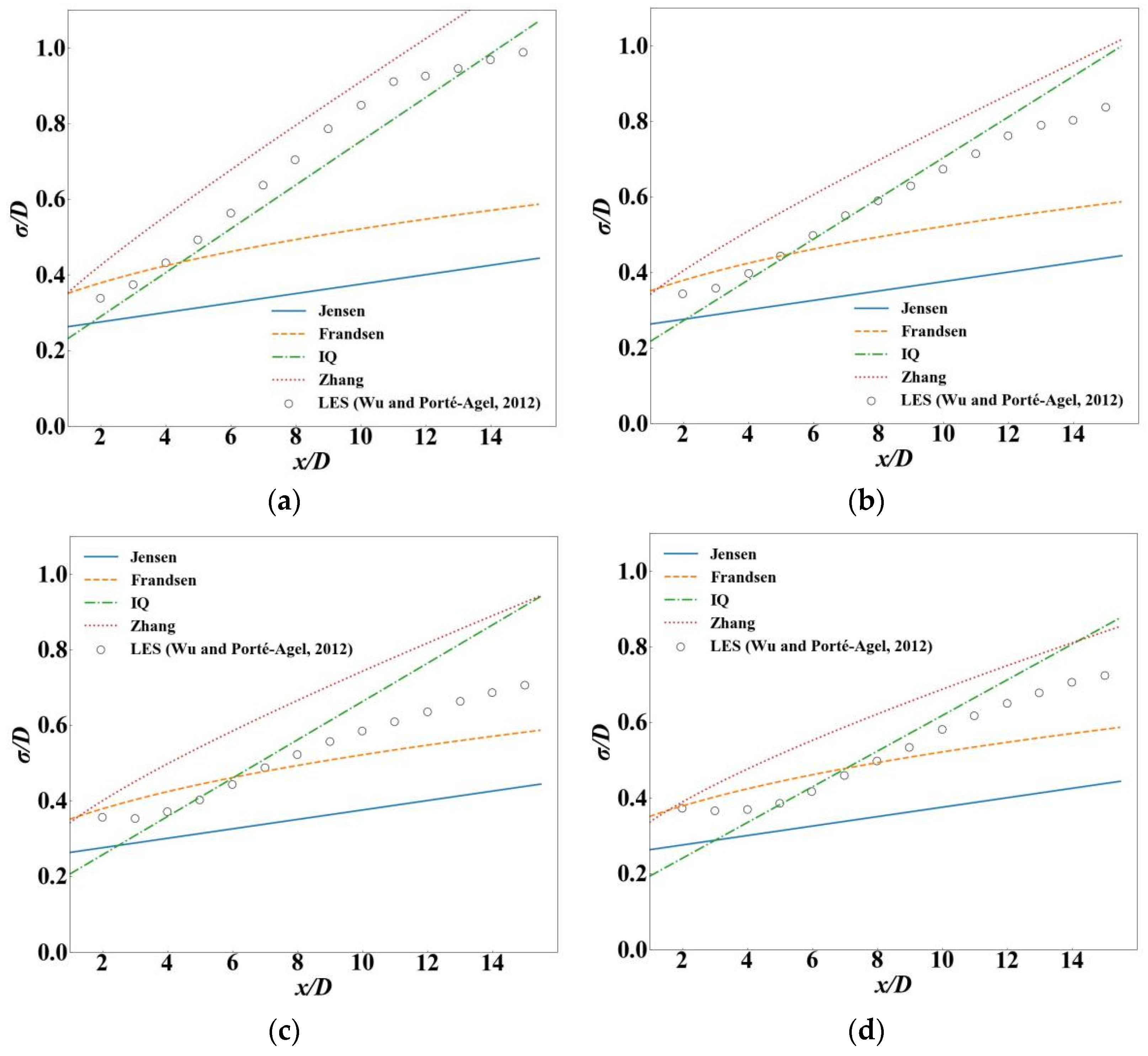
Numerical simulations [29] were carried out to study the effects of ambient turbulence intensity on turbine wake structures and the wake boundary expansions along the downstream distances were calculated. Four cases with different ambient turbulence intensities of 0.134, 0.094, 0.069, and 0.048 were studied. The wake boundary expansions predicted by different models are compared with the numerical simulations [29] in Figure 2. The wake boundary predictions by the Jensen model and the Frandsen model are not influenced by the ambient turbulence intensity, and they maintain the same trend for four cases. It seems that they are parallel with each other when the thrust coefficient is equal to 0.8, although the wake boundary curve predicted by the Frandsen model is non-linear. In addition, the curves predicted that the IQ model shows acceptable agreement with numerical simulations for all the cases, while the results by the Zhang model are always slightly larger than numerical simulations. The Frandsen model provides an acceptable result only if the ambient turbulence intensity is low, while the Jensen model shows the worst result. Therefore, the linear and non-linear wake boundary expansion models proposed by Ishihara and Qian [5], Zhang et al. [7], and Frandsen et al. [3] are considered in the following contents due to their advantages.

2.3. Added Turbulence Intensity

The added turbulence intensity will be generated by the rotating blades of the upcoming turbine and they will affect the wake boundary expansion. The higher added turbulence intensity will accelerate the flow mixing with surrounding air. Table 3 summarizes four empirical wake models to describe the streamwise added turbulence intensity. The more advanced wake models to evaluate the added turbulence intensity considering the spanwise distribution are not considered in this study.
Figure 3 illustrates comparison of the streamwise distribution of added turbulence intensity between numerical simulations [5] and empirical models. It is noted that the results by the Crespo and Hernandez model, by the Larsen model, and by IEC model show good agreement with simulations in Figure 3b, in Figure 3c, and Figure 3d, respectively. Compared with other empirical models, the Larsen mode presents acceptable results for all cases. Furthermore, the streamwise added turbulence intensities predicted by the Crespo and Hernandez model and the Larsen model change more smoothly with the downstream distance and they are close to each other. The other two curves by the Frandsen model and the IEC 61400-1 model have the same trends, while the streamwise added turbulence intensity predicted by the IEC 61400-1 model has a higher value. Predictions of the streamwise added turbulence intensity converge in the far wake region, except in the Frandsen model.
The turbulence intensity in the wake region can be separated into two parts: the ambient turbulence intensity and the added turbulence intensity. Three superposition approaches are used in the previous studies to generate the turbulence intensity in Table 4. The added turbulence intensity should be modified slightly based on different superposition approaches and the detailed explanations can be found in the references [23,33].

2.4. Summary of the Wake Models

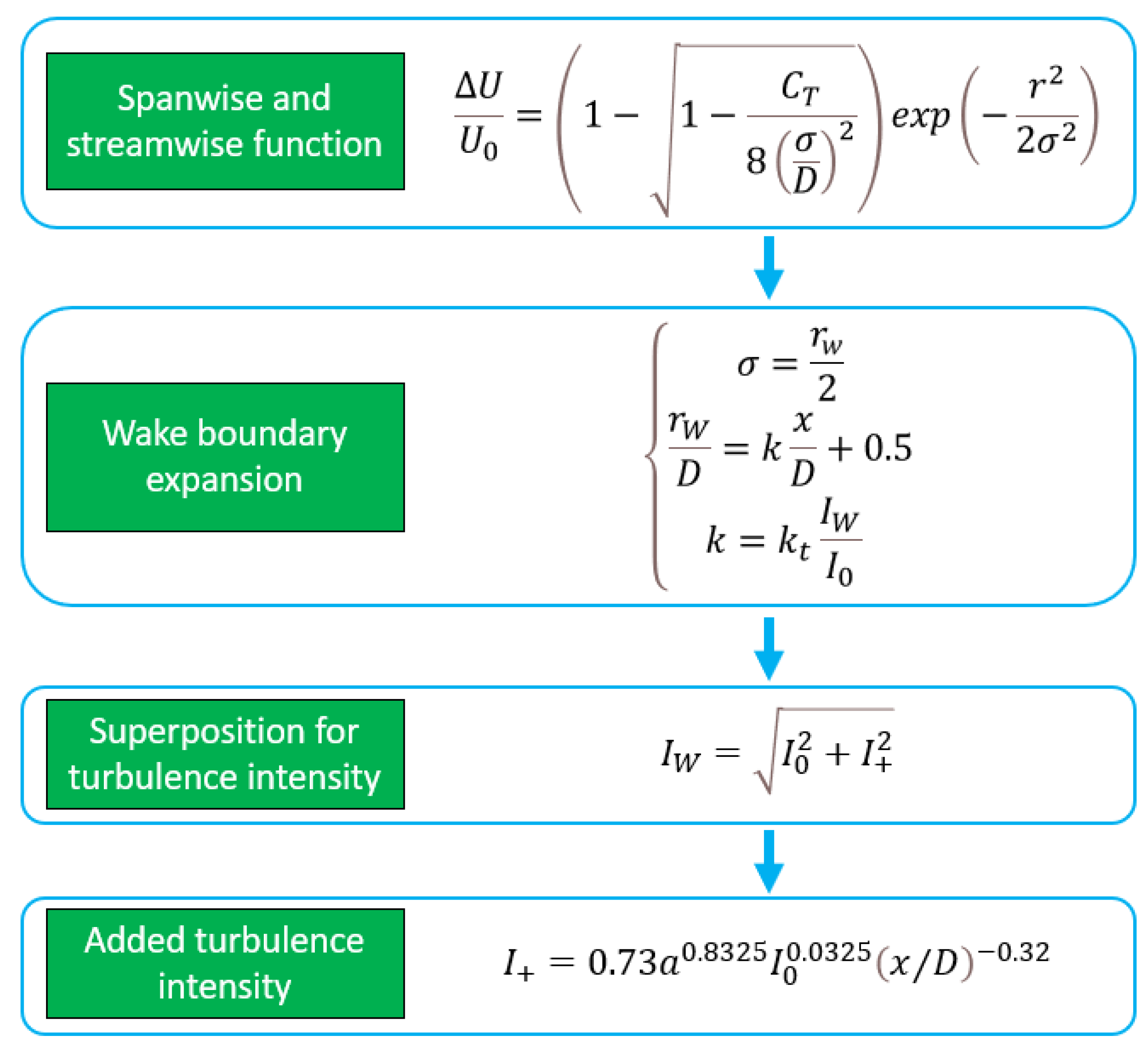
Wake models for the single wind turbine are summarized in this section. As shown in Figure 4, an example of the combined wake model is introduced. The spanwise and streamwise functions are chosen in Table 1. At this moment, it is necessary to calculate wake boundary expansion which cannot derived by the mass and momentum equations. Either the linear or the non-linear empirical models in Table 2 can be used. The added turbulence intensity and the superposition methods for turbulence intensity are selected in Table 3 and in Table 4, respectively, if the non-linear empirical model is adopted. The wake model has been finished if the linear empirical model is chosen. Finally, the combined wake model is proposed. In this study, 70 combined wake models are totally proposed and summarized, including wake models proposed by other researchers, such as the BP model, IQ model, Zhang model, Yang model etc., in Table A1.

3. Wake Models for Multiple Wind Turbines

The superposition approaches to add the wake velocity deficit for multiple wind turbines are presented in Section 3.1 and the Horn Rev 1 offshore wind farm is illustrated in Section 3.2.

3.1. Superposition Approaches

Six superposition approaches are commonly used to add the wake velocity deficit in Table 5. For the ambient-based velocity deficit superposition approach, it is assumed that the space between two wind turbines is large and their interaction between each other can be negligible, so that the inflow velocity of the downstream wind turbine and the whole wind farm are close to each other, i.e., u h , i u 0 . For the rotor-based velocity deficit superposition approach, the velocity deficit over the whole rotor area of the downstream turbine is not uniform, so the averaged inflow velocity over the whole rotor area is calculated by Equation (9). The velocity deficit can be added together by the linear sum method or the root sum square method. For the energy deficit linear sum method, the square of velocity is considered as a scalar and be summed linearly. It should be pointed out that these six superposition approaches are empirical methods without a rigorous theoretical foundation. It is expected that the rotor-based velocity deficit superposition approach is more accurate, especially for the cases with short turbine spacing, since it avoids the error accumulation of inflow wind velocity from upstream to downstream [15,16].
Wake superposition effects of two wind turbines are shown in Figure 5. It is assumed that the wake velocity deficit generated by the upstream wind turbine (red line) will be superposed to the downstream wake velocity deficit (blue line) and the final velocity deficit is illustrated as the black line.
U h , i = A 0 U d A
where U shows the wake velocity at the ith wind turbine in a wind farm.

3.2. Horn Rev 1 Wind Farm

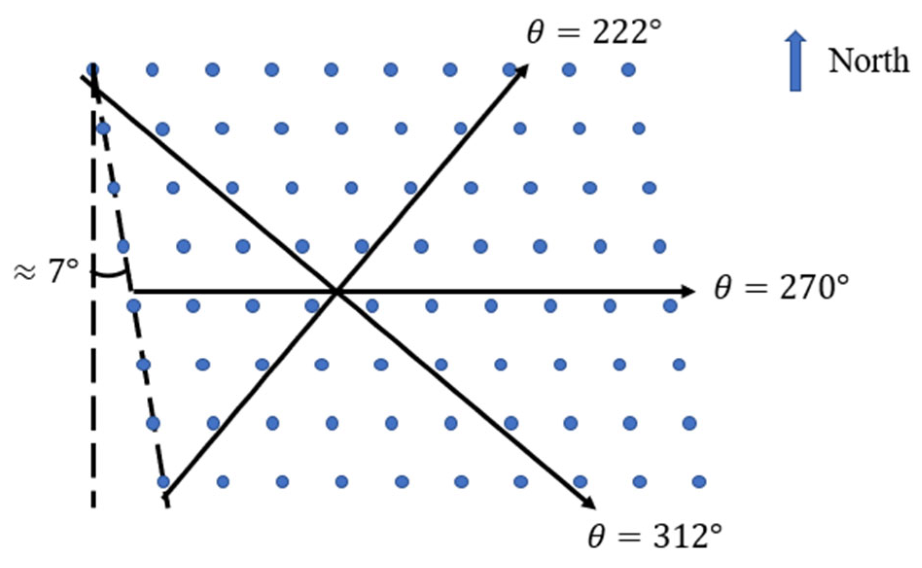
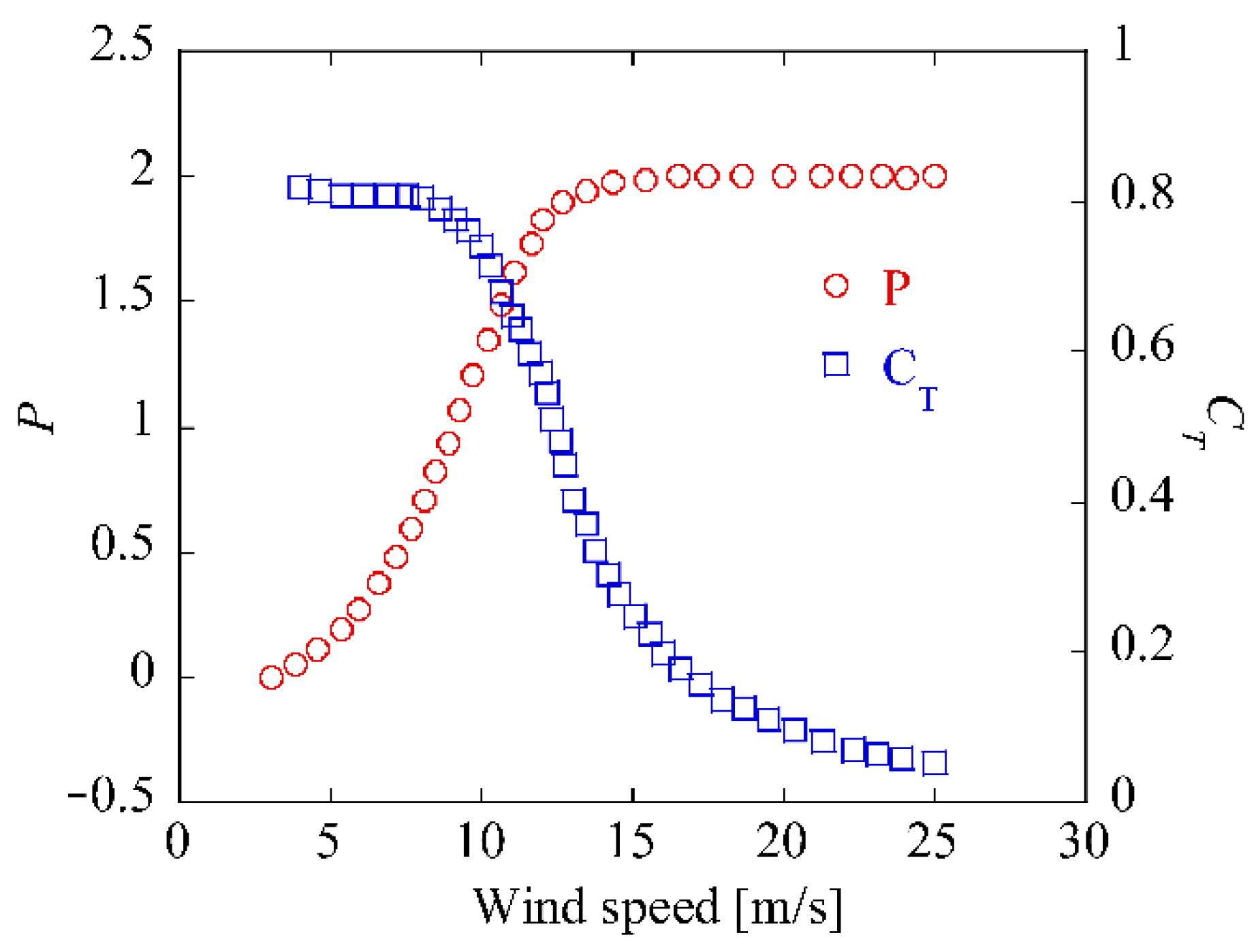
The Horns Rev offshore wind farm is situated in the eastern North Sea in Denmark, and the first phase, consisting of 80 Vestas V-80 2 MW wind turbines (Horns Rev 1), was operated in 2002. The whole wind farm has a rhomboid distribution and the layout of wind turbines is illustrated in Figure 6. Basic parameters of the wind turbine, including the rotor diameter, the hub height, and the cut-in and cut-off velocities are provided by the manufacturer and shown in Table 6. The thrust coefficient C T and power curves P are illustrated in Figure 7 and the specific values at a special inflow wind velocity are calculated by the linear interpolation method. The operational conditions are also shown in Table 6, i.e., the inflow velocity, the ambient turbulence intensity, and the aerodynamic surface roughness.
The wake models for multiple wind turbines are validated by numerical simulations carried out by Wu and Porte-Agel [35] where the turbine wake and power loss of the Horns Rev 1 offshore wind farm are numerically studied.

4. Results and Discussions

The combined wake models for both single and multiple wind turbines are proposed and validated by numerical and experimental results in Section 4.1 and in Section 4.2, respectively. Effects of thrust coefficient and ambient turbulence intensity are studied in Section 4.3 and in Section 4.4, respectively.

4.1. Single Wind Turbine

To propose a wake model for predictions of velocity deficit, the spanwise distributions and wake boundary expansion models should be determined. The added turbulence intensity models and the superposition approaches for turbulence intensity should also be taken into account if the nonlinear wake boundary expansion model is used. In this study, modified wake models combined by different spanwise distributions mentioned in Section 2.1 with different wake boundary expansion models introduced in Section 2.2 are proposed to improve the accuracy and versatility. There are in total 70 combined wake models, and these are shown in the Appendix A in Table A1.
To validate the combined wake models, a series of numerical simulations, wind tunnel tests, and field tests were summarized from the previous studies and the basic parameters of measurements and simulations, including ambient turbulence intensity, thrust coefficient, aerodynamic surface roughness, hub height, rotor diameter, and normalized downstream distances are shown in Table 7. The aerodynamic surface roughness z 0 for simulations carried out by Ishihara and Qian is unknown, and they are defined as the same values with simulations by Wu and Porté-Agel [29] due to the similar ambient turbulence intensity.
In general, to validate the wake model, a specific case with the known thrust coefficient and ambient turbulence intensity is considered, and the measurement and prediction data at a special downstream distance in the spanwise direction are compared. In this study, a comprehensive comparison is conducted to validate every combined wake model where all the measurements in Table 7 are used. To prevent the redundant comparisons between predictions and case-by-case measurements, we put all the prediction and measurement data in one figure and the hit rate q [38] is adopted as index to quantitatively evaluate the accuracy and versatility of combined wake models. It is expressed as follows:
q = 1 N t i = 1 N t n i       w i t h       n i = { 1                             | p i m i m i | D q     o r     | p i m i | W q 0                                                                                                                             e l s e    
where m i and p i refer to measurements and predictions data for a special value i . N t presents the total number of prediction data. The threshold values are followed by the German VDI guideline 3783-9 where D q = 0.25 and W q = 0.07 | m a x | [39].
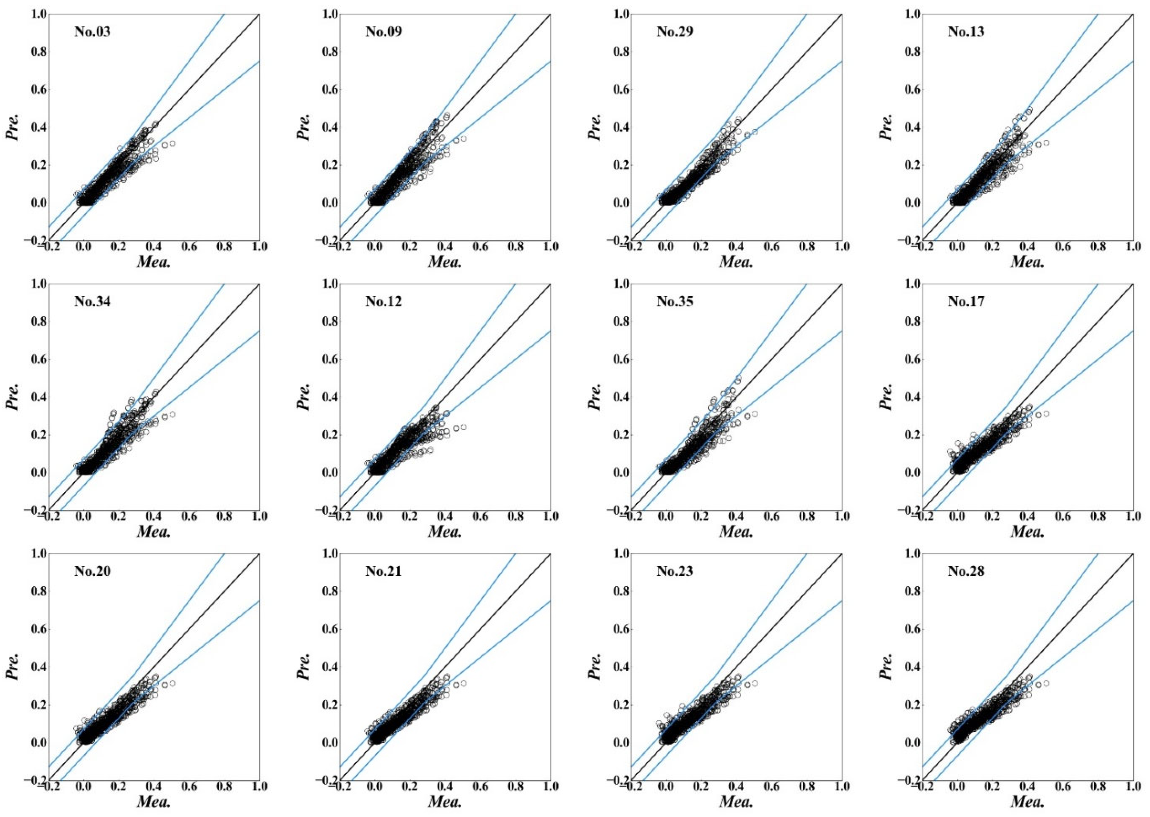
The velocity deficit at the hub height in the spanwise direction at different downstream distances for every case in Table 7 is used to compute the hit rate. The combined wake models with the top 12 highest hit rates are listed in Table 8 and comparisons between predictions by combined wake models and measurements are illustrated in Figure 8. The blue lines show the threshold values followed by the German VDI guideline 3783-9 [39]. It is obvious that most points fall within the threshold range for the No. 3, No. 9, No. 29, and No. 13 combined wake models which means they have the higher hit rate. It was found that the No. 3 [7] and No. 9 wake models have the highest hit rate with q = 0.92, which means that the wake models are more universal than others. It was interesting to find that, compared with the IQ model (No. 15) by Ishihara and Qian [5], the No. 29 wake model combining the streamwise function by Bastankhah and Porté-Agel [4] with the linear wake boundary expansion model by Ishihara and Qian [5] had a higher hit rate.

4.2. Multi Wind Turbines

Wind farms generally consist of tens or hundreds of wind turbines to improve the efficiency of wind power generation. To accurately evaluate turbine wakes and power loss for multiple turbines, it is necessary to properly combine the single wake model and the superposition approach.
In this section, 70 combined wake models for the single wind turbine mentioned above will be checked whether they can be adopted to evaluate turbine wakes in wind farms and the proper superposition approach will also be chosen to combine with the single turbine wake model. Numerical simulations of turbine wakes in a row carried out by Wu and Porté-Agel [35] were used to validate the combination method. To save time and effort, the inflow wind velocity of the second wind turbine was firstly calculated by the single turbine wake model and the process would be stopped if the inflow wind velocity was far different from the numerical results. On the contrary, the single turbine wake model accompanied with different superposition approaches was considered to calculate the wind velocity, turbulence intensity, and power generation of every wind turbine in a row. It was observed that predictions by the following five models for multiple wind turbines match well with simulations, while results predicted by other models are either underestimated or overestimated and they are not shown in this manuscript.
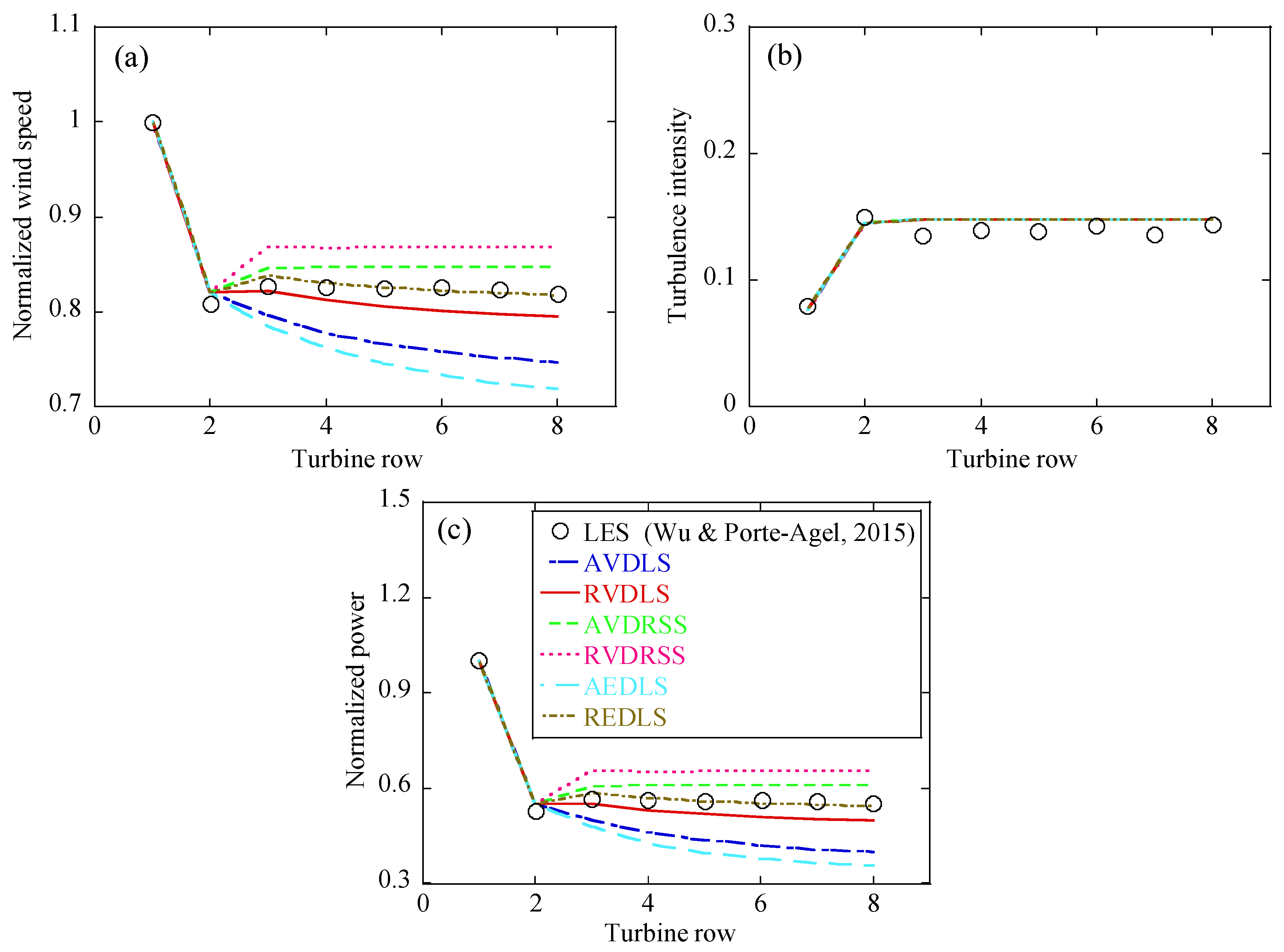
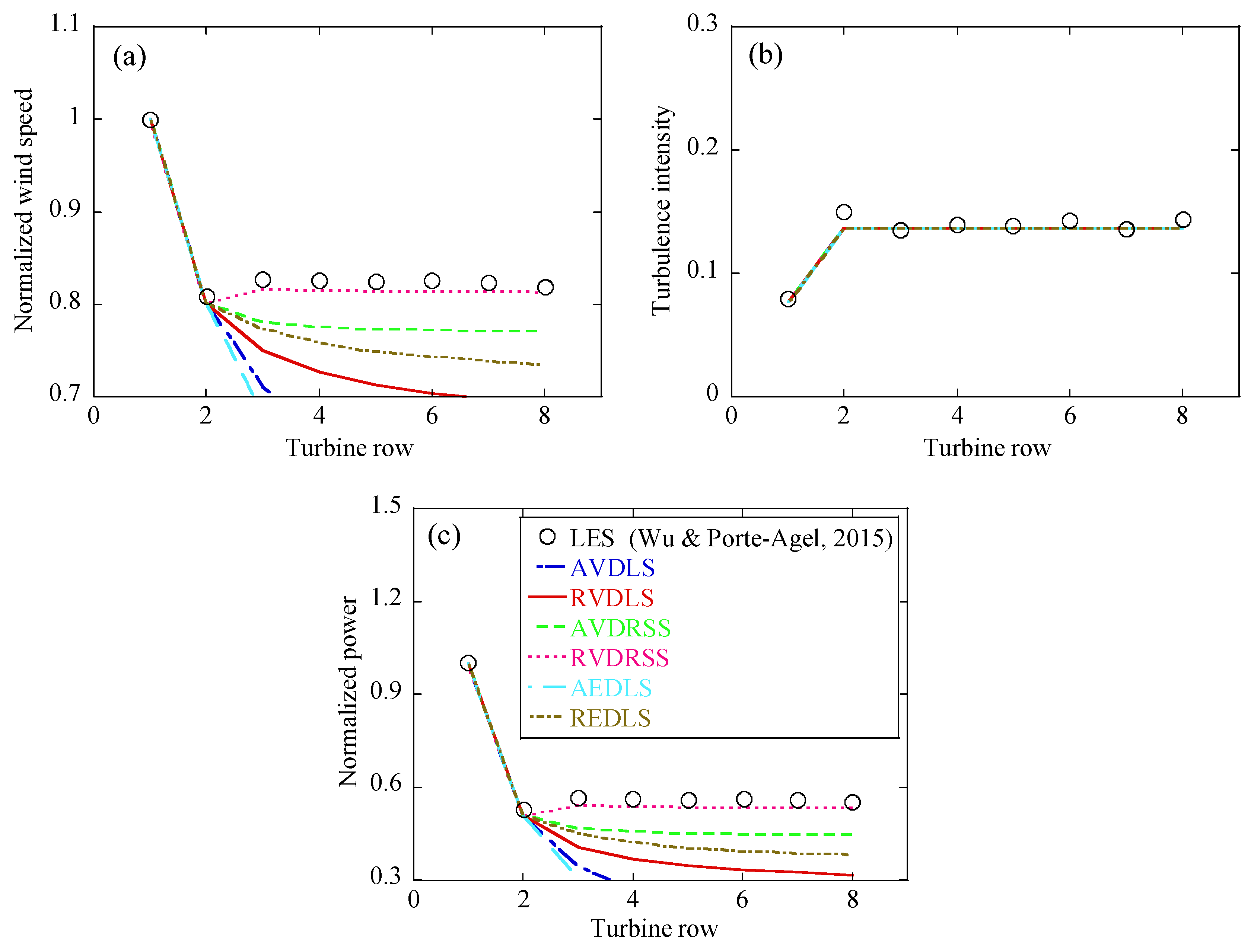
Figure 9 illustrates comparisons of velocity deficit, turbulence intensity, and power generation between simulation and prediction results by the No. 29 combined wake model with different superposition approaches. The wind speed and power generation are normalized by the inflow wind velocity and the wind power generation by the first wind turbine, respectively. It is noted that the rotor-based energy deficit linear superposition approach is more suitable for the No. 29 combined wake model and the predicted results show excellent agreement with simulations. However, the predicted results are either overestimated or underestimated by other superposition approaches. As for the turbulence intensity, the Crespo and Hernandez model is adopted and the added turbulence intensity induced by the closest upwind turbine is considered. As shown in Figure 10, the results by the No. 37 combined wake model with the rotor-based velocity deficit root sum square approach matches well with numerical simulations. In summary, both the No. 29 and the No. 37 combined wake models show their good performance for predictions of turbine-induced velocity deficit, turbulence intensity, and wind power generation in a wind farm.
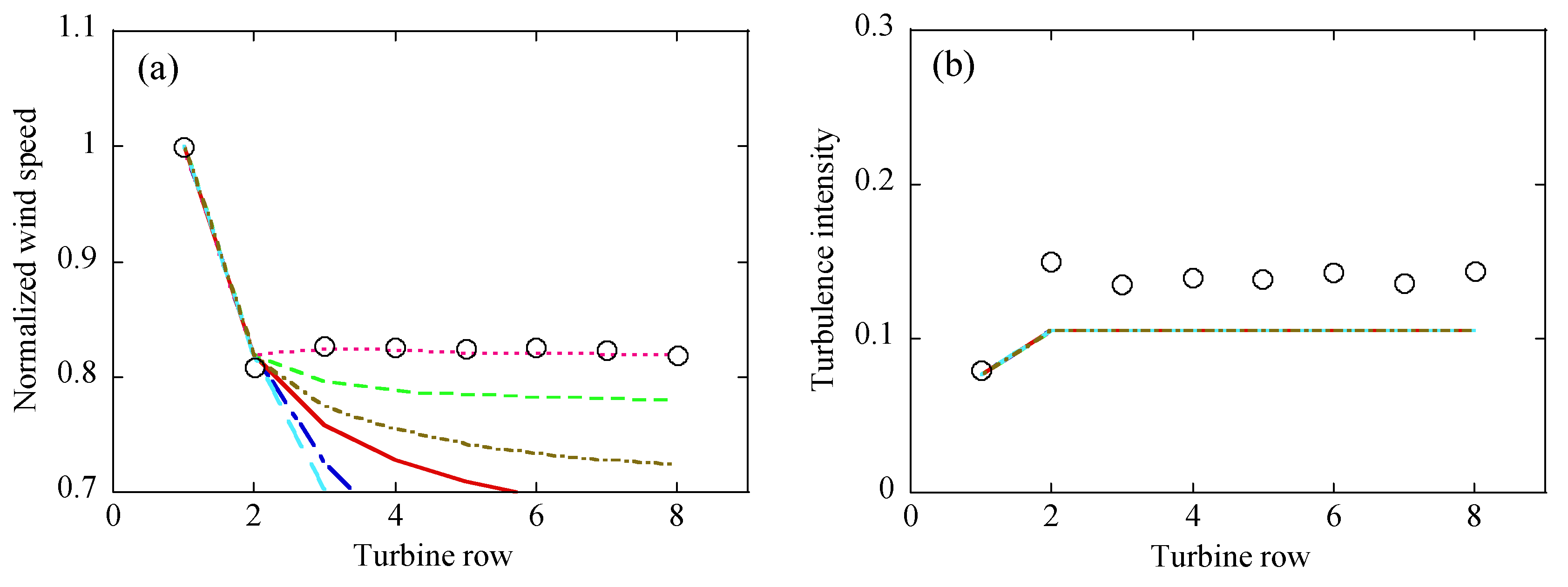
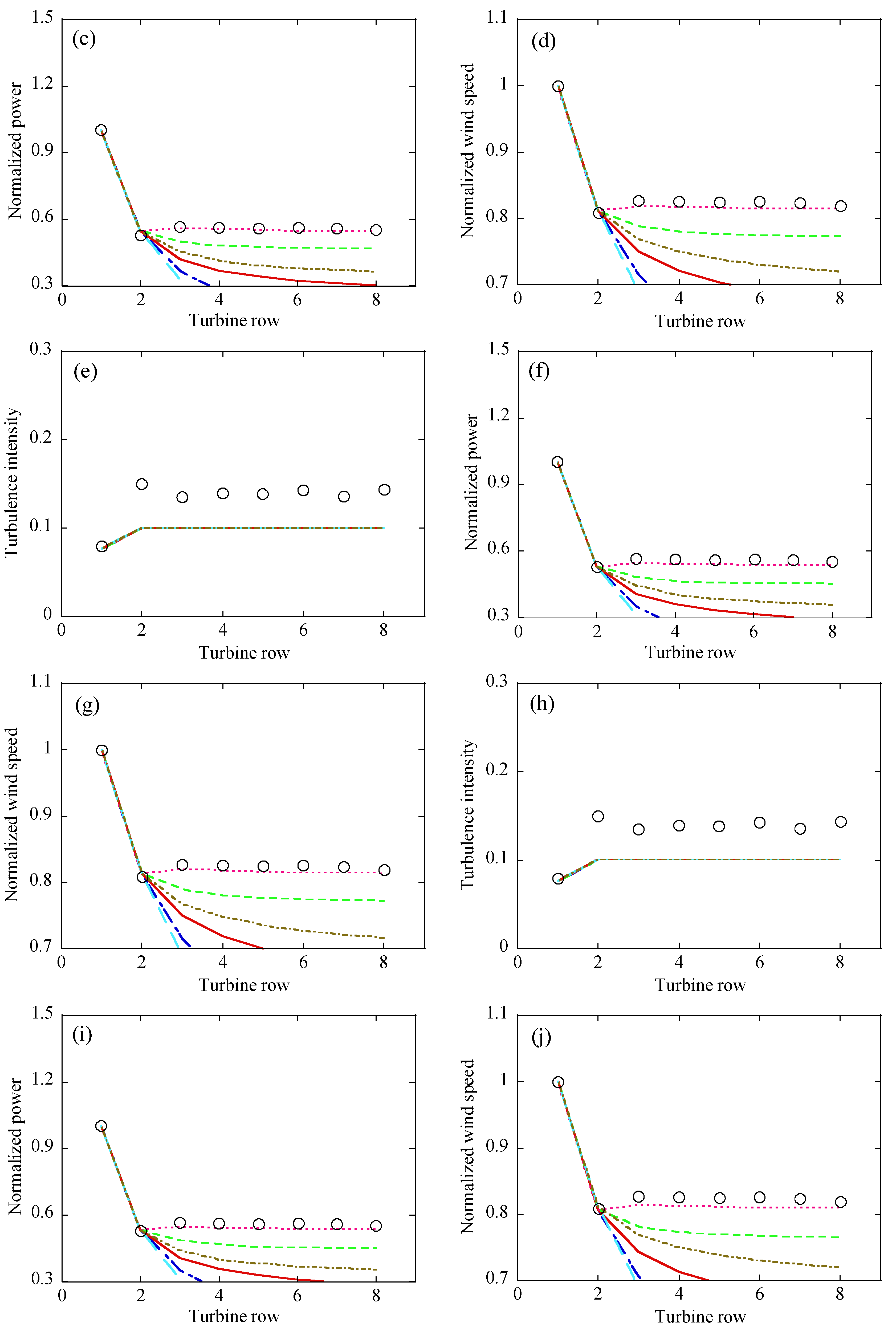
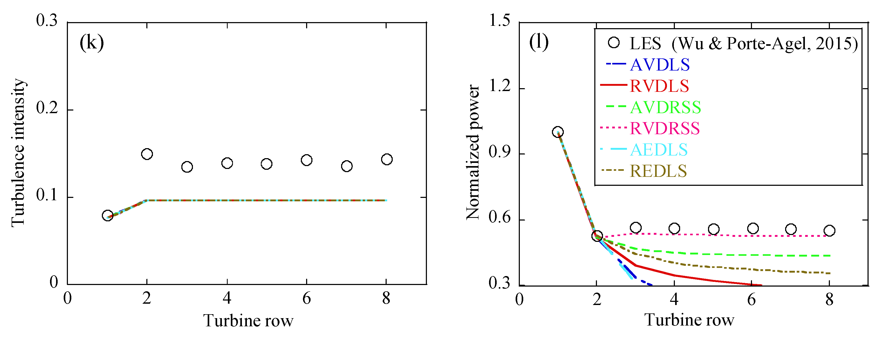
It is also noted that predictions by the ambient-based energy deficit linear sum approach are the smallest, while results by the rotor-based velocity deficit root sum square approach are the largest in Figure 9, Figure 10 and Figure 11. The rotor-based energy deficit linear sum and the rotor-based velocity deficit linear sum approaches are moderate. In fact, prediction errors by wake models always exist and these errors may be accumulated by the superposition approaches. Therefore, it is necessary to choose the wake model and the superposition approach properly. In this study, it is recommended that the No. 29 combined wake model and the rotor-based energy deficit linear sum approach.
In addition, it is interesting to note that turbine-induced velocity deficit and wind power generation for multiple turbines in a row can be accurately predicted by the top-hat type wake models, including the No. 46, No. 47, No. 52, and No. 53 combined wake models while the turbulence intensities are underestimated as illustrated in Figure 11. The top-hat type wake models cannot accurately evaluate the velocity deficit for a single wind turbine since spanwise distributions are different from measured wake data and they maintain the same value over the whole rotor area. However, they neglect the process to calculate the equivalent velocity as shown in Equation (9) which may induce some errors.

4.3. Effect of Thrust Coefficient

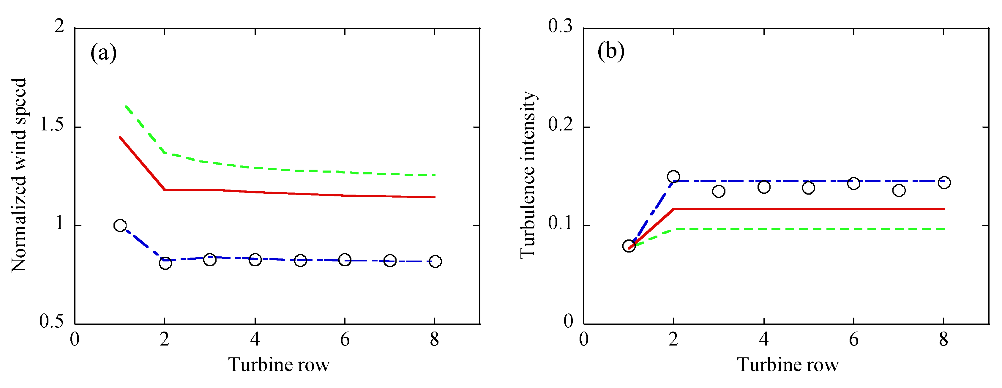
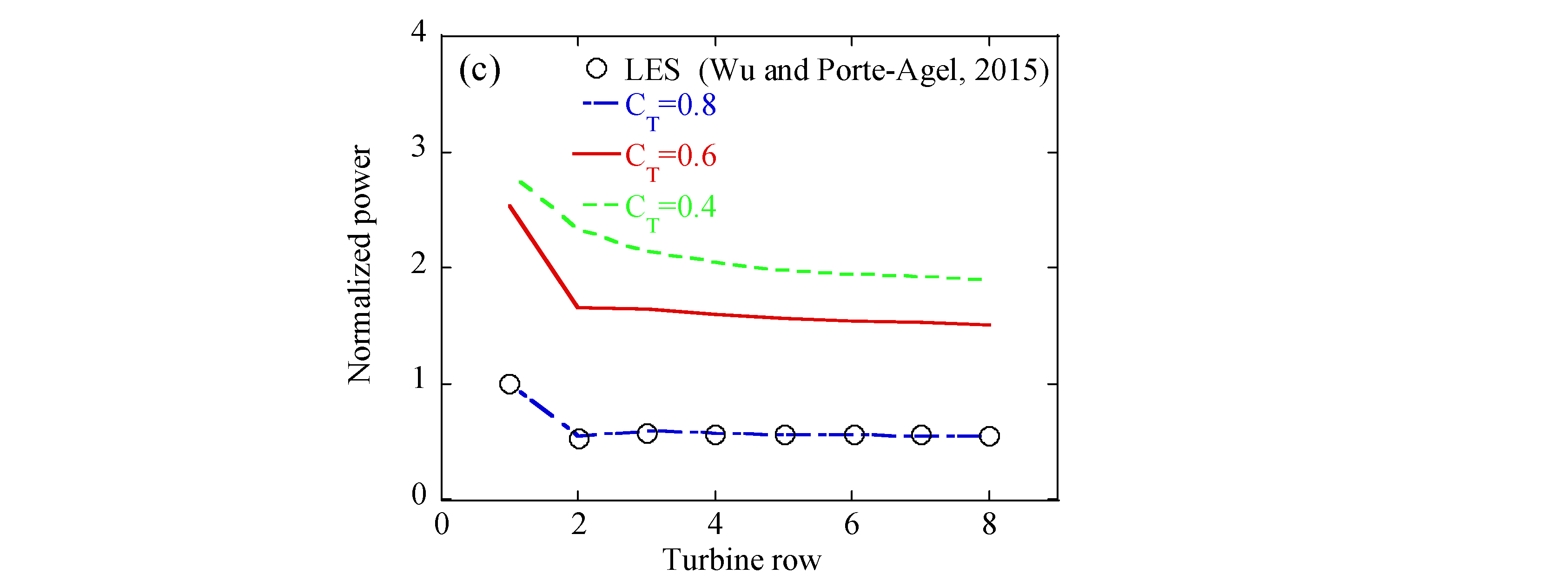
The thrust coefficient has an essential influence on the wake boundary expansion and velocity deficit. Simultaneously, it is determined by the inflow velocity at hub height as shown in Figure 7. In a wind farm, the inflow wind velocity cannot be a constant value, and it always changes in nature. Therefore, it is necessary to discuss the effect of thrust coefficient on the velocity, turbulence intensity, and power generation for multiple turbines in a row.
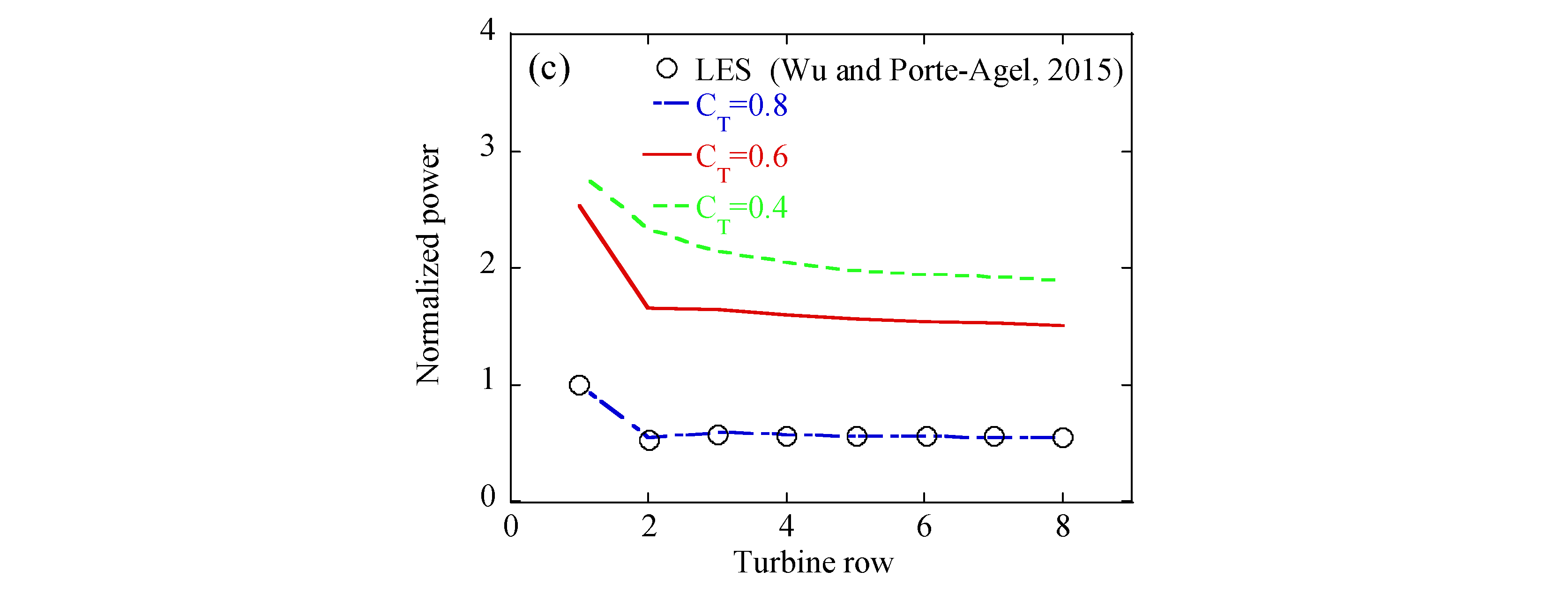
Three different thrust coefficients including C T = 0.8 , C T = 0.6 and C T = 0.4 , are discussed in this study, and the corresponding inflow velocities at the hub height are U 0 = 8   m / s , U 0 = 11.6   m / s and U 0 = 13.1   m / s . The ambient turbulence intensity and aerodynamic surface roughness maintain the same values with the numerical simulations [35].
Figure 12 shows the velocity, turbulence intensity, and power generation of multiple wind turbines in a row by the No. 29 combined wind turbine and the rotor-based energy deficit linear sum approach under different thrust coefficients. It is obvious that the wind velocity and wind power generation will increase as the thrust coefficient decreases mainly because the inflow wind speed rises. The normalized wind velocity and power generation are normalized by the inflow wind speed and the power generation of the first wind turbine when the thrust coefficient is 0.8. They have the same variation trend along the downstream distance as the thrust coefficient changes. As for the turbulence intensity, it decreases as the thrust coefficient decreases. At this moment, the wind speed can pass through the turbine disk easily due to the reduction of thrust coefficient and turbulence generated by blades decreases accordingly. In fact, the thrust coefficient is not an independent parameter and it is determined by the inflow wind velocity at the hub height. Therefore, the effects of inflow wind velocity and thrust coefficient are studied together.

4.4. Effect of Ambient Turbulence Intensity

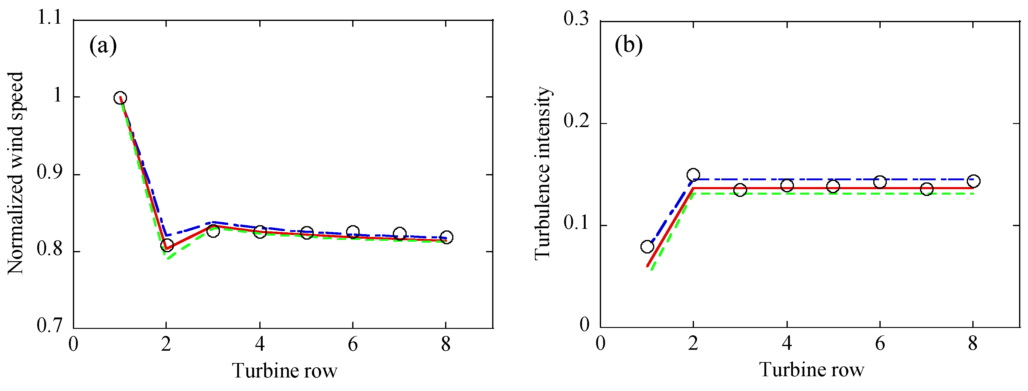
The ambient turbulence intensity affects the flow mixing in the wake region and the wake boundary expansion. For offshore wind farms, the wind speed is stable and the ambient turbulence intensity is generally low, but it will still vary slightly. Therefore, three ambient turbulence intensities, namely I 0 = 0.05 , I 0 = 0.06 , and I 0 = 0.077 , are considered in this section. At this moment, other parameters will not be changed.
The effect of ambient turbulence intensity on velocity, turbulence intensity, and power generation of multiple wind turbines is studied as illustrated in Figure 13. The No. 29 combined wake model and the rotor-based energy deficit linear sum approach are used as well. It is observed that the ambient turbulence intensity has slight effects on the turbine-induced velocity deficit, turbulence intensity, and wind power generation in Figure 13 since its variation is limited. In fact, the downstream wind speed in front of the second wind turbine increases slightly as the ambient turbulence intensity rises due to the acceleration of flow mixing. The ambient turbulence intensity is an independent ambient parameter which will not be affected by the inflow wind velocity and the turbine condition. It is assumed that the ambient turbulence intensity maintains around 5% in the offshore wind farm. At this moment, the wind velocity and power generation will scarcely be affected by the ambient turbulence intensity.

5. Concluding Remarks

This paper investigated the applicability of wake models to predict turbine-induced velocity deficits and wind power generations for both single and multi-wind turbines. The conclusions are summarized as follows:
  • A series of wake models for a single wind rubine are proposed by combining different spanwise distributions and wake boundary expansion models. Compared with measurement data, the top 12 wake models ranked by the hit rate are summarized and they are more universal and accurate than others, especially for the No. 3, No. 9, and No. 29 combined wake models, which are considered as the most suitable wake models for the single wind turbine.
  • The wake models for multiple wind turbines are proposed by considering combined wake models for the single wind turbine and six superposition approaches. It is recommended that the No. 29 wake model combined with the rotor-based energy deficit linear superposition approach and the No. 37 wake model combined with the rotor-based velocity deficit root sum square approach should be used to carry out wind farm layout optimization due to their accurate predictions of velocity, turbulence intensity, and power generation for multiple wind turbines.
  • The effects of thrust coefficient and ambient turbulence intensity on the velocity, turbulence intensity, and wind power generation are investigated. It is found that the wind velocity as well as wind power generation increase, and the turbulence intensity decreases as the thrust coefficient reduces, whilst they almost maintain the same value as the ambient turbulence intensity varies.

Author Contributions

Conceptualization, G.H. and D.Z.; methodology, G.H. and D.Z.; software, D.Z. and Y.L.; validation, D.Z. and Y.L.; formal analysis, D.Z. and Y.L.; investigation, D.Z.; resources, G.H.; data curation, D.Z.; writing—original draft preparation, D.Z. and Y.L.; writing—review and editing, D.Z., G.H. and C.L.; visualization, D.Z. and Y.L.; supervision, G.H., C.L. and Y.X.; project administration, G.H.; funding acquisition, G.H. All authors have read and agreed to the published version of the manuscript.

Funding

This study is supported by National Key R&D Program of China (2021YFC3100702), National Natural Science Foundation of China (52108451), Shenzhen Science and Technology Innovation Commission (SGDX20210823103202018, GXWD20201230155427003-20200823230021001), Shenzhen Key Laboratory Launching Project (ZDSYS20200810113601005), and Guangdong-Hong Kong-Macao Joint Laboratory for Data-Driven Fluid Mechanics and Engineering Applications (2020B1212030001).

Conflicts of Interest

The authors declare no conflict of interest.

Nomenclature

aaxial flow induction factor
a1parameter in IQ model
A0cross-sectional area of rotor
AWcross-sectional area of downwind wake
bparameter in IQ model
cparameter in IQ model
CTthrust coefficient
C(x)streamwise function of outside Gaussian flow for velocity deficit
Drotor diameter
Dqfirst threshold of hit rate
DWwake diameter downwind of the rotor
G(r)spanwise functions of velocity deficit
I+added turbulence intensity
I0ambient turbulence intensity
Iwwake turbulence intensity
kwake expansion rate in the far wake region
Kconstant in Frandsen model
Knempirical constant in Frandsen model
ktthe constant rate of wake expansion
kwmodified wake expansion rate in Zhang model
mimeasured data
nthe total number of wind turbines
Ntthe total number of prediction data
Pwind power
Pipredicted data
qhit rate
rradial distance from rotor center
r0rotor radius
r1/2half width of the wake
r w wake boundary at one special streamwise distance
Uwake velocity
Uh,ithe inflow velocity for ith wind turbine at hub height
Uithe wake velocity of the ith wind turbine
U0inflow wind velocity
UWstreamwise velocity downwind of the rotor
Wqsecond threshold of hit rate
xstreamwise distance downstream wind turbine
yspanwise distance downstream wind turbine
z 0 surface roughness length
zhthe turbine hub height
Greek Symbols
α empirical constant in Frandsen model
β wake expansion parameter in Frandsen model
ε intercept in IQ model
I streamwise function of the added turbulence intensity
U i wake velocity deficit of the ith wind turbine
U wake velocity deficit
U m a x wake velocity deficit at hub height
θ wind angle
ρ air density
σ standard deviation of Gaussian wake velocity deficit

Appendix A

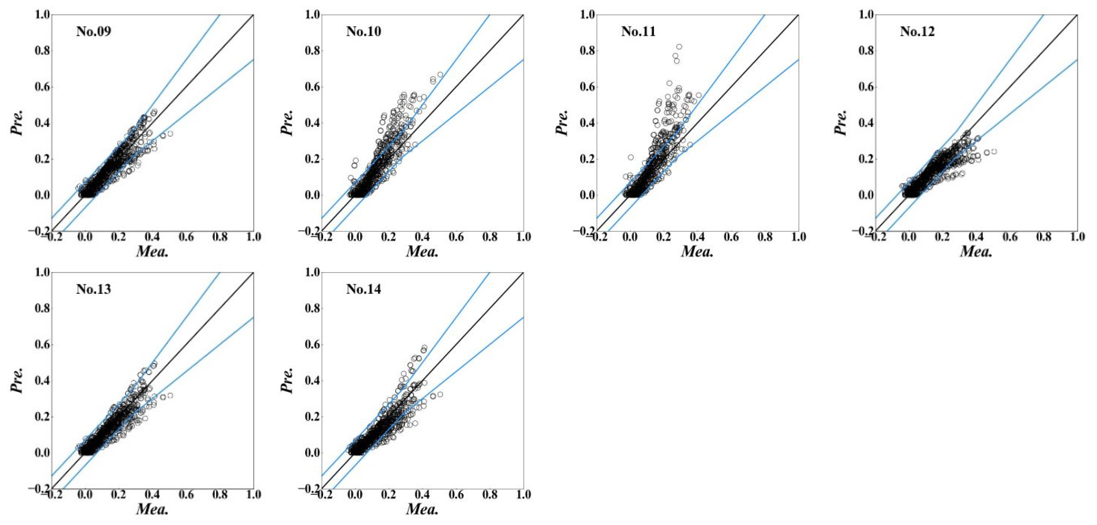
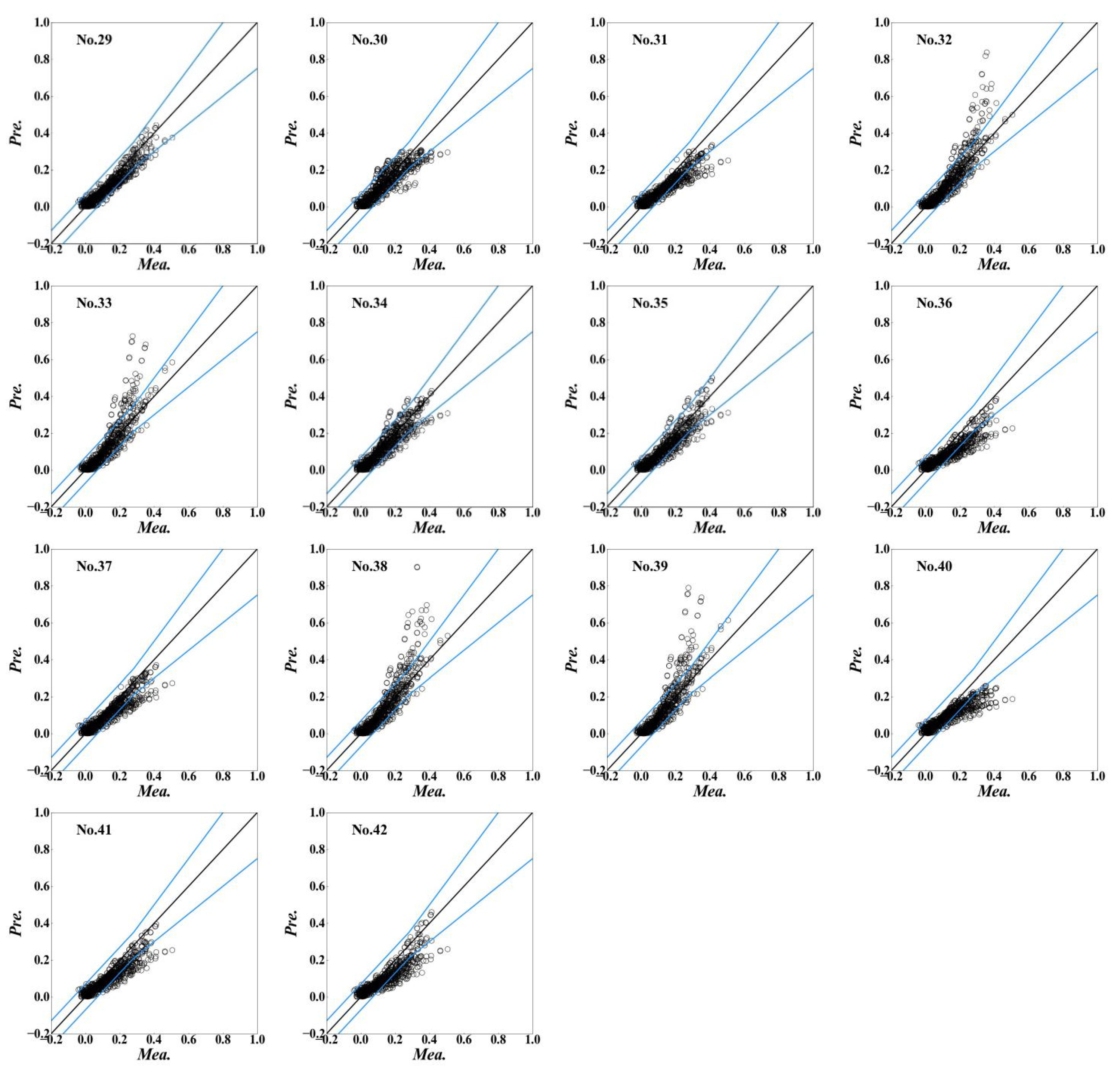
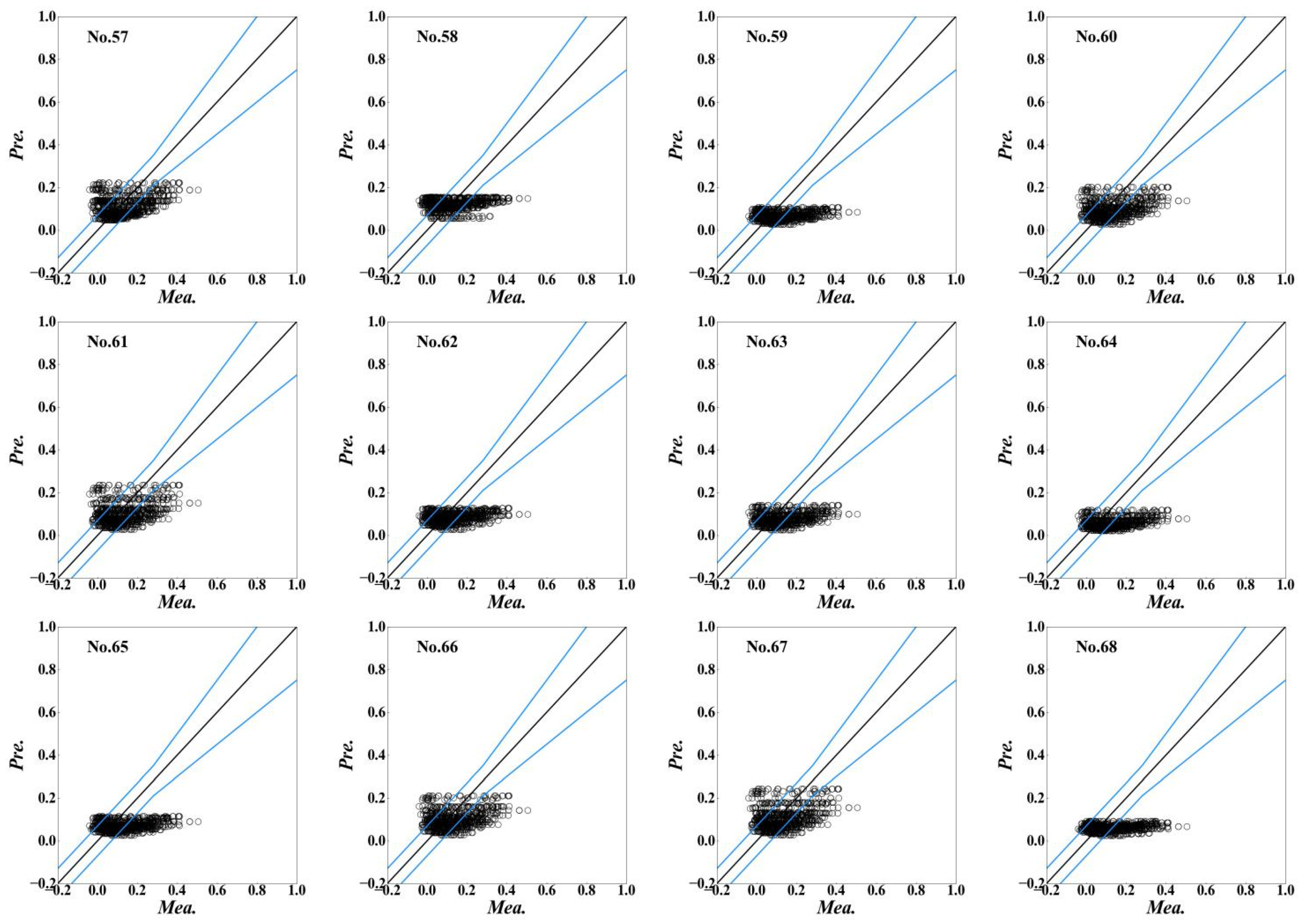
All the combined wake models are shown in Table A1 considering different spanwise distributions, streamwise functions, wake boundary expansion models, added turbulence intensity models, and the superposition approaches for turbulence intensity. The hit rate q for every combined wake model is calculated by comparing prediction and measurement data. To provide a comprehensive comparison, the wake models proposed by previous studies have also been added in Table A1, such as the No. 3 [7], No. 15 [5], No. 34 [13], and No. 58 [3] wake models. The comparisons of the combined wake models are shown in Figure A1, Figure A2, Figure A3, Figure A4 and Figure A5. For the single wind turbine, it is obviously noted that combined wake models with Gaussian and cosine-shaped distributions have high hit rates, which mean they can be used to accurately predict the turbine-induced velocity deficit while the models with the top-hat distribution have low hit rates since the spanwise distributions are different from measurement data.
Table A1. Descriptions of the combined wake models.
CaseSpanwise DistributionStreamwise FunctionWake Boundary ExpansionAdded Turbulence IntensityTurbulence IntensityHit Rate
1CosineZhang modelLinear (IQ)--0.55
2CosineZhang modelNon-linear (F)--0.48
3CosineZhang modelNon-linear (Z)Crespo and Hernandez modelSquare and root0.92
4CosineZhang modelNon-linear (Z)Crespo and Hernandez modelLinear sum0.68
5CosineZhang modelNon-linear (Z)Crespo and Hernandez modelRoot and square0.64
6CosineZhang modelNon-linear (Z)Frandsen modelSquare and root0.82
7CosineZhang modelNon-linear (Z)Frandsen modelLinear sum0.87
8CosineZhang modelNon-linear (Z)Frandsen modelRoot and square0.87
9CosineZhang modelNon-linear (Z)Larsen modelSquare and root0.92
10CosineZhang modelNon-linear (Z)Larsen modelLinear sum0.64
11CosineZhang modelNon-linear (Z)Larsen modelRoot and square0.61
12CosineZhang modelNon-linear (Z)IEC modelSquare and root0.89
13CosineZhang modelNon-linear (Z)IEC modelLinear sum0.9
14CosineZhang modelNon-linear (Z)IEC modelRoot and square0.87
15GaussianIQ modelLinear (IQ)--0.85
16GaussianIQ modelNon-linear (F)--0.85
17GaussianIQ modelNon-linear (Z)Crespo and Hernandez modelSquare and root0.88
18GaussianIQ modelNon-linear (Z)Crespo and Hernandez modelLinear sum0.87
19GaussianIQ modelNon-linear (Z)Crespo and Hernandez modelRoot and square0.86
20GaussianIQ modelNon-linear (Z)Frandsen modelSquare and root0.88
21GaussianIQ modelNon-linear (Z)Frandsen modelLinear sum0.88
22GaussianIQ modelNon-linear (Z)Frandsen modelRoot and square0.87
23GaussianIQ modelNon-linear (Z)Larsen modelSquare and root0.88
24GaussianIQ modelNon-linear (Z)Larsen modelLinear sum0.87
25GaussianIQ modelNon-linear (Z)Larsen modelRoot and square0.86
26GaussianIQ modelNon-linear (Z)IEC modelSquare and root0.86
27GaussianIQ modelNon-linear (Z)IEC modelLinear sum0.87
28GaussianIQ modelNon-linear (Z)IEC modelRoot and square0.88
29GaussianBP modelLinear (IQ)--0.91
30GaussianBP modelNon-linear (F)--0.87
31GaussianBP modelNon-linear (Z)Crespo and Hernandez modelSquare and root0.84
32GaussianBP modelNon-linear (Z)Crespo and Hernandez modelLinear sum0.84
33GaussianBP modelNon-linear (Z)Crespo and Hernandez modelRoot and square0.76
34GaussianBP modelNon-linear (Z)Frandsen modelSquare and root0.9
35GaussianBP modelNon-linear (Z)Frandsen modelLinear sum0.89
36GaussianBP modelNon-linear (Z)Frandsen modelRoot and square0.76
37GaussianBP modelNon-linear (Z)Larsen modelSquare and root0.85
38GaussianBP modelNon-linear (Z)Larsen modelLinear sum0.81
39GaussianBP modelNon-linear (Z)Larsen modelRoot and square0.75
40GaussianBP modelNon-linear (Z)IEC modelSquare and root0.76
41GaussianBP modelNon-linear (Z)IEC modelLinear sum0.82
42GaussianBP modelNon-linear (Z)IEC modelRoot and square0.79
43Top-hatJensen modelLinear (IQ)--0.47
44Top-hatJensen modelNon-linear (F)--0.45
45Top-hatJensen modelNon-linear (Z)Crespo and Hernandez modelSquare and root0.46
46Top-hatJensen modelNon-linear (Z)Crespo and Hernandez modelLinear sum0.48
47Top-hatJensen modelNon-linear (Z)Crespo and Hernandez modelRoot and square0.47
48Top-hatJensen modelNon-linear (Z)Frandsen modelSquare and root0.48
49Top-hatJensen modelNon-linear (Z)Frandsen modelLinear sum0.48
50Top-hatJensen modelNon-linear (Z)Frandsen modelRoot and square0.46
51Top-hatJensen modelNon-linear (Z)Larsen modelSquare and root0.47
52Top-hatJensen modelNon-linear (Z)Larsen modelLinear sum0.47
53Top-hatJensen modelNon-linear (Z)Larsen modelRoot and square0.47
54Top-hatJensen modelNon-linear (Z)IEC modelSquare and root0.47
55Top-hatJensen modelNon-linear (Z)IEC modelLinear sum0.47
56Top-hatJensen modelNon-linear (Z)IEC modelRoot and square0.45
57Top-hatFrandsen modelLinear (IQ)--0.45
58Top-hatFrandsen modelNon-linear (F)--0.48
59Top-hatFrandsen modelNon-linear (Z)Crespo and Hernandez modelSquare and root0.46
60Top-hatFrandsen modelNon-linear (Z)Crespo and Hernandez modelLinear sum0.46
61Top-hatFrandsen modelNon-linear (Z)Crespo and Hernandez modelRoot and square0.47
62Top-hatFrandsen modelNon-linear (Z)Frandsen modelSquare and root0.48
63Top-hatFrandsen modelNon-linear (Z)Frandsen modelLinear sum0.47
64Top-hatFrandsen modelNon-linear (Z)Frandsen modelRoot and square0.46
65Top-hatFrandsen modelNon-linear (Z)Larsen modelSquare and root0.46
66Top-hatFrandsen modelNon-linear (Z)Larsen modelLinear sum0.47
67Top-hatFrandsen modelNon-linear (Z)Larsen modelRoot and square0.47
68Top-hatFrandsen modelNon-linear (Z)IEC modelSquare and root0.48
69Top-hatFrandsen modelNon-linear (Z)IEC modelLinear sum0.46
70Top-hatFrandsen modelNon-linear (Z)IEC modelRoot and square0.44
Linear (IQ), Non-linear (F) and Non-linear (Z): the linear or nonlinear wake boundary expansion models proposed by Ishihara and Qian [5]; by Frandsen et al. [3]; by Zhang et al. [7].
Figure A1. Comparisons of the combined wake models with the cosine-shaped distribution.
Energies 15 07431 g0a1aEnergies 15 07431 g0a1b
Figure A2. Comparisons of the combined wake models with the Gaussian distribution and the streamwise distribution of IQ model.
Energies 15 07431 g0a2
Figure A3. Comparisons of the combined wake models with the Gaussian distribution and the streamwise distribution of BP model.
Energies 15 07431 g0a3
Figure A4. Comparisons of the combined wake models with the top-hat distribution and the streamwise distribution of Jensen model.
Energies 15 07431 g0a4aEnergies 15 07431 g0a4b
Figure A5. Comparisons of the combined wake models with the top-hat distribution and the streamwise distribution of Frandsen model.
Energies 15 07431 g0a5aEnergies 15 07431 g0a5b

References

  1. GWEC. Global Wind Report 2021; Global Wind Energy Council: Brussels, Belgium, 2021. [Google Scholar]
  2. Jensen, N.O. A Note on Wind Generator Interaction; Risø National Laboratory: Roskilde, Denmark, 1983. [Google Scholar]
  3. Frandsen, S.; Barthelmie, R.; Pryor, S.; Rathmann, O.; Larsen, S.; Højstrup, J.; Thøgersen, M. Analytical Modelling of Wind Speed Deficit in Large Offshore Wind Farms. Wind Energ. 2006, 9, 39–53. [Google Scholar] [CrossRef]
  4. Bastankhah, M.; Porté-Agel, F. A New Analytical Model for Wind-Turbine Wakes. Renew. Energy 2014, 70, 116–123. [Google Scholar] [CrossRef]
  5. Ishihara, T.; Qian, G.-W. A New Gaussian-Based Analytical Wake Model for Wind Turbines Considering Ambient Turbulence Intensities and Thrust Coefficient Effects. J. Wind Eng. Ind. Aerodyn. 2018, 177, 275–292. [Google Scholar] [CrossRef]
  6. Tian, L.; Zhu, W.; Shen, W.; Zhao, N.; Shen, Z. Development and Validation of a New Two-Dimensional Wake Model for Wind Turbine Wakes. J. Wind Eng. Ind. Aerodyn. 2015, 137, 90–99. [Google Scholar] [CrossRef] [Green Version]
  7. Zhang, Z.; Huang, P.; Sun, H. A Novel Analytical Wake Model with a Cosine-Shaped Velocity Deficit. Energies 2020, 13, 3353. [Google Scholar] [CrossRef]
  8. Gao, X.; Li, B.; Wang, T.; Sun, H.; Yang, H.; Li, Y.; Wang, Y.; Zhao, F. Investigation and Validation of 3D Wake Model for Horizontal-Axis Wind Turbines Based on Filed Measurements. Appl. Energy 2020, 260, 114272. [Google Scholar] [CrossRef]
  9. Sun, H.; Yang, H. Study on an Innovative Three-Dimensional Wind Turbine Wake Model. Appl. Energy 2018, 226, 483–493. [Google Scholar] [CrossRef]
  10. Ge, M.; Wu, Y.; Liu, Y.; Yang, X.I.A. A Two-Dimensional Jensen Model with a Gaussian-Shaped Velocity Deficit. Renew. Energy 2019, 141, 46–56. [Google Scholar] [CrossRef]
  11. Keane, A. Advancement of an Analytical Double-Gaussian Full Wind Turbine Wake Model. Renew. Energy 2021, 171, 687–708. [Google Scholar] [CrossRef]
  12. Wang, Y.; Lin, J.; Zhang, J. Investigation of a New Analytical Wake Prediction Method for Offshore Floating Wind Turbines Considering an Accurate Incoming Wind Flow. Renew. Energy 2022, 185, 827–849. [Google Scholar] [CrossRef]
  13. Yang, Q.; Li, H.; Li, T.; Zhou, X. Wind Farm Layout Optimization for Levelized Cost of Energy Minimization with Combined Analytical Wake Model and Hybrid Optimization Strategy. Energy Convers. Manag. 2021, 248, 114778. [Google Scholar] [CrossRef]
  14. Pillai, A.C.; Chick, J.; Khorasanchi, M.; Barbouchi, S.; Johanning, L. Application of an Offshore Wind Farm Layout Optimization Methodology at Middelgrunden Wind Farm. Ocean Eng. 2017, 139, 287–297. [Google Scholar] [CrossRef] [Green Version]
  15. Kirchner-Bossi, N.; Porté-Agel, F. Realistic Wind Farm Layout Optimization through Genetic Algorithms Using a Gaussian Wake Model. Energies 2018, 11, 3268. [Google Scholar] [CrossRef] [Green Version]
  16. Qian, G.-W.; Ishihara, T. Wind Farm Power Maximization through Wake Steering with a New Multiple Wake Model for Prediction of Turbulence Intensity. Energy 2021, 220, 119680. [Google Scholar] [CrossRef]
  17. Lissaman, P.B.S. Energy Effectiveness of Arbitrary Arrays of Wind Turbines. J. Energy 1979, 3, 323–328. [Google Scholar] [CrossRef]
  18. Niayifar, A.; Porté-Agel, F. Analytical Modeling of Wind Farms: A New Approach for Power Prediction. Energies 2016, 9, 741. [Google Scholar] [CrossRef] [Green Version]
  19. Katic, I.; Højstrup, J.; Jensen, N.O. A Simple Model for Cluster Efficiency. In EWEC’86. Proceedings; European Wind Energy Association: Rome, Italy, 1987; pp. 407–410. [Google Scholar]
  20. Voutsinas, S. On the Analysis of Wake Effects in Wind Parks. Wind Eng. 1990, 14, 204–219. [Google Scholar]
  21. Göçmen, T.; van der Laan, P.; Réthoré, P.-E.; Diaz, A.P.; Larsen, G.C.; Ott, S. Wind Turbine Wake Models Developed at the Technical University of Denmark: A Review. Renew. Sustain. Energy Rev. 2016, 60, 752–769. [Google Scholar] [CrossRef] [Green Version]
  22. Shao, Z.; Wu, Y.; Li, L.; Han, S.; Liu, Y. Multiple Wind Turbine Wakes Modeling Considering the Faster Wake Recovery in Overlapped Wakes. Energies 2019, 12, 680. [Google Scholar] [CrossRef] [Green Version]
  23. Tian, L.; Zhu, W.; Shen, W.; Song, Y.; Zhao, N. Prediction of Multi-Wake Problems Using an Improved Jensen Wake Model. Renew. Energy 2017, 102, 457–469. [Google Scholar] [CrossRef]
  24. Barthelmie, R.J.; Larsen, G.C.; Frandsen, S.T.; Folkerts, L.; Rados, K.; Pryor, S.C.; Lange, B.; Schepers, G. Comparison of Wake Model Simulations with Offshore Wind Turbine Wake Profiles Measured by Sodar. J. Atmos. Ocean. Technol. 2006, 23, 888–901. [Google Scholar] [CrossRef]
  25. Barthelmie, R.J.; Jensen, L.E. Evaluation of Wind Farm Efficiency and Wind Turbine Wakes at the Nysted Offshore Wind Farm. Wind Energy 2010, 13, 573–586. [Google Scholar] [CrossRef]
  26. Cleve, J.; Greiner, M.; Enevoldsen, P.; Birkemose, B.; Jensen, L. Model-Based Analysis of Wake-Flow Data in the Nysted Offshore Wind Farm. Wind Energy 2009, 12, 125–135. [Google Scholar] [CrossRef]
  27. Barthelmie, R.J.; Frandsen, S.T.; Nielsen, M.N.; Pryor, S.C.; Rethore, P.-E.; Jørgensen, H.E. Modelling and Measurements of Power Losses and Turbulence Intensity in Wind Turbine Wakes at Middelgrunden Offshore Wind Farm. Wind Energy 2007, 10, 517–528. [Google Scholar] [CrossRef]
  28. Ge, M.; Wu, Y.; Liu, Y.; Li, Q. A Two-Dimensional Model Based on the Expansion of Physical Wake Boundary for Wind-Turbine Wakes. Appl. Energy 2019, 233–234, 975–984. [Google Scholar] [CrossRef]
  29. Wu, Y.-T.; Porté-Agel, F. Atmospheric Turbulence Effects on Wind-Turbine Wakes: An LES Study. Energies 2012, 5, 5340–5362. [Google Scholar] [CrossRef] [Green Version]
  30. Crespo, A.; Hernández, J. Turbulence Characteristics in Wind-Turbine Wakes. J. Wind Eng. Ind. Aerodyn. 1996, 61, 71–85. [Google Scholar] [CrossRef]
  31. Larsen, G.C.; Højstrup, J.; Madsen, H.A. Wind Fields in Wakes. In Proceedings of the 1996 European Wind Energy Conference and Exhibition, Göteborg, Sweden, 20–24 May 1996. [Google Scholar]
  32. IEC 61400-1; Wind Turbine Generator Systems Part 1: Safety Requirements. International Electrotechnical Commission: Geneva, Switzerland, 2019.
  33. Gao, X.; Yang, H.; Lu, L. Optimization of Wind Turbine Layout Position in a Wind Farm Using a Newly-Developed Two-Dimensional Wake Model. Appl. Energy 2016, 174, 192–200. [Google Scholar] [CrossRef]
  34. Renkema, D.J. Validation of Wind Turbine Wake Models. Master’s Thesis, TU Delft, Delft, The Netherlands, 2007. [Google Scholar]
  35. Wu, Y.-T.; Porté-Agel, F. Modeling Turbine Wakes and Power Losses within a Wind Farm Using LES: An Application to the Horns Rev Offshore Wind Farm. Renew. Energy 2015, 75, 945–955. [Google Scholar] [CrossRef]
  36. Schreiber, J.; Balbaa, A.; Bottasso, C.L. Brief Communication: A Double-Gaussian Wake Model. Wind Energ. Sci. 2020, 5, 237–244. [Google Scholar] [CrossRef] [Green Version]
  37. Bastankhah, M.; Porté-Agel, F. A New Miniature Wind Turbine for Wind Tunnel Experiments. Part II: Wake Structure and Flow Dynamics. Energies 2017, 10, 923. [Google Scholar] [CrossRef]
  38. Oettl, D. Quality Assurance of the Prognostic, Microscale Wind-Field Model GRAL 14.8 Using Wind-Tunnel Data Provided by the German VDI Guideline 3783-9. J. Wind Eng. Ind. Aerodyn. 2015, 142, 104–110. [Google Scholar] [CrossRef]
  39. VDI. Environmental Meteorology—Prognostic Microscale Windfield Models—Evaluation for Flow around Buildings and Obstacles; Tech. Rep., VDI guideline 3783, Part 9; Beuth Verlag: Berlin, Germany, 2005. [Google Scholar]
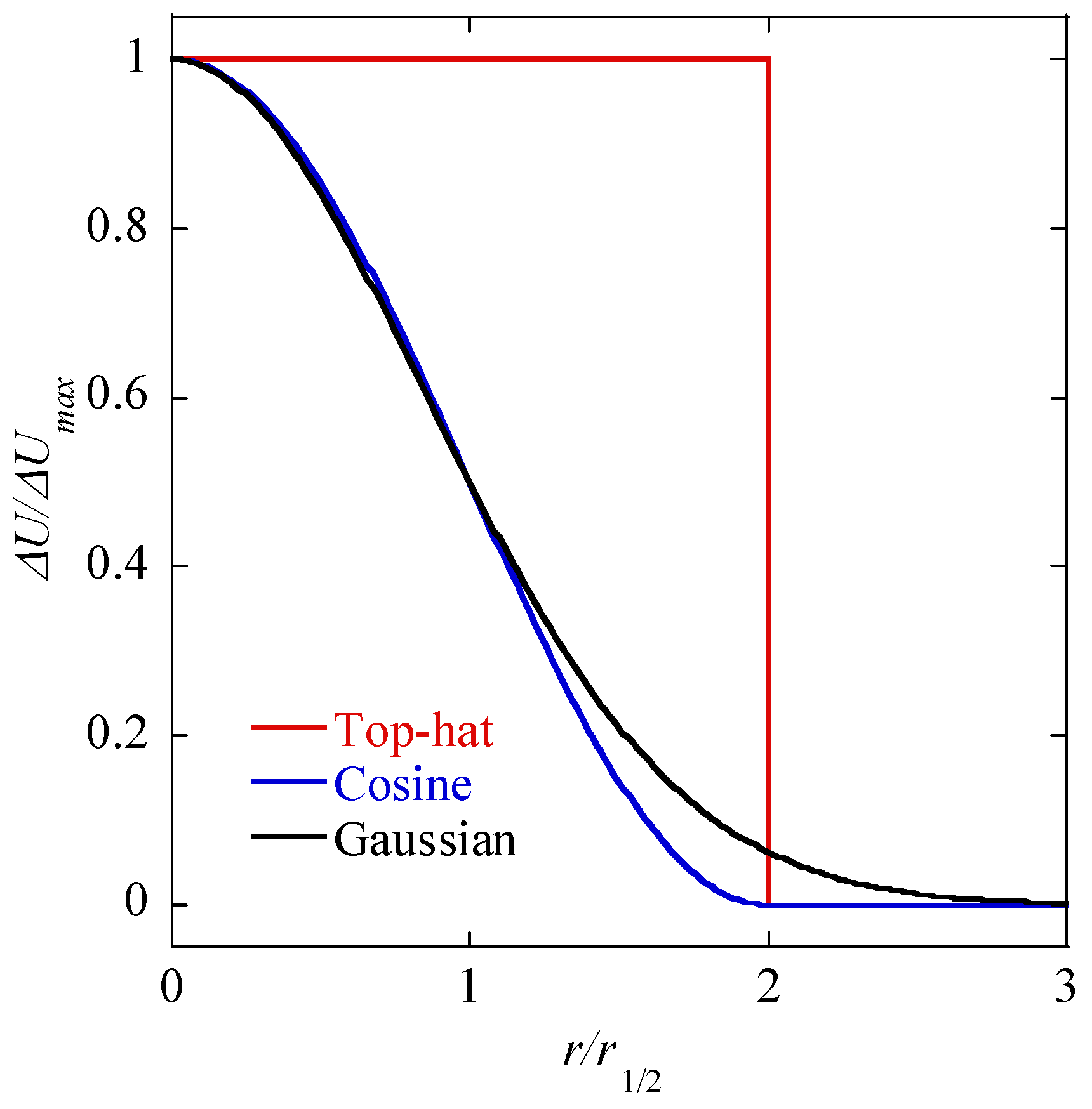
Figure 1. Spanwise distribution of velocity deficit.
Energies 15 07431 g001
Figure 2. Comparisons of the wake boundary expansion between numerical simulations ( C T = 0.8 ,   z h = 70   m ) [4] and the empirical models: (a) I 0 = 0.134 ,   z 0 = 0.5   m ; (b) I 0 = 0.094 ,   z 0 = 0.05   m ; (c) I 0 = 0.069 ,   z 0 = 0.005   m ; (d) I 0 = 0.048 ,   z 0 = 0.00005   m .
Energies 15 07431 g002
Figure 3. Comparison of the streamwise distributions of added turbulence intensity between numerical simulations [5] and empirical models: (a) I 0 = 0.035 ,   C T = 0.36 ; (b) I 0 = 0.035 ,   C T = 0.84 ; (c) I 0 = 0.137 ,   C T = 0.36 ; (d) I 0 = 0.137 ,   C T = 0.84 .
Energies 15 07431 g003
Figure 4. An example of the combined wake model.
Energies 15 07431 g004
Figure 5. Wake superposition effect of two wind turbines.
Energies 15 07431 g005
Figure 6. Wind turbine layout of the Horn Rev 1 wind farm.
Energies 15 07431 g006
Figure 7. Thrust coefficient C T and power curves P of the wind turbine [35].
Energies 15 07431 g007
Figure 8. Comparison between predictions by combined wake models and measurements (blue line: threshold values; black line: Mea. = Pre; dot: velocity deficit).
Energies 15 07431 g008
Figure 9. Comparisons of: (a) velocity deficit; (b) turbulence intensity; (c) power generations between simulations and predictions by the No. 29 combined wake model with different superposition approaches.
Energies 15 07431 g009
Figure 10. Comparisons of: (a) velocity deficit; (b) turbulence intensity; (c) power generations between simulations and predictions by the No. 37 combined wake model with different superposition approaches.
Energies 15 07431 g010
Figure 11. Comparisons of velocity deficit, turbulence intensity and power generations between simulations and predictions by: (ac) the No. 46 combined wake model; (df) the No. 47 combined wake model; (gi) the No. 52 combined wake model; (jl) the No. 53 combined wake model; with different superposition approaches.
Energies 15 07431 g011aEnergies 15 07431 g011bEnergies 15 07431 g011c
Figure 12. Effect of thrust coefficient on: (a) wind velocity; (b) turbulence intensity; (c) wind power generation of wind turbines in a row.
Energies 15 07431 g012aEnergies 15 07431 g012b
Figure 13. Effect of ambient turbulence intensity on: (a) wind velocity; (b) turbulence intensity; (c) wind power generation of wind turbines in a row.
Energies 15 07431 g013aEnergies 15 07431 g013b
Table 1. Analytical and empirical wake models in the far wake region.
ModelExpressionWake Boundary ExpansionApplication
Jensen [2] U U 0 = ( 1 1 C T ) ( D D w ) 2 LinearWFLO [23]
Frandsen et al. [3] U U 0 = 1 2 ( 1 1 2 A A w C T ) Non-linearN/A
Bastankhah and Porté-Agel [4] U U 0 = ( 1 1 C T 8 ( σ D ) 2 ) e x p ( r 2 2 σ 2 ) LinearWFLO [22]
Ishihara and Qian [5] U U 0 = C T [ a 1 + b x D + c ( 1 + x D ) 2 ] 2 e x p ( r 2 2 σ 2 ) LinearWind farm power generation [20]
Zhang et al. [7] U U 0 = [ π 2 4 3 π 2 16 ( π 2 4 3 π 2 16 ) 2 π 2 C T 3 π 2 16 ( r 0 r w ) 2 ] × [ c o s ( r r w π ) + 1 ] Non-linearN/A
Table 2. Empirical models for wake boundary expansion.
RefPrincipleExpressionParameters
Jensen [2]Linear D W D = k x D + 1 k = 0.05
Frandsen et al. [3]Non-linear D W D = ( β K 2 + α x D ) 1 K α = 0.7
K = 3
β = 1 + 1 C T 2 1 C T
Ishihara and Qian [5]Linear σ D = k x D + ε k = 0.11 C T 1.07 I 0 0.2
ε = 0.23 C T 0.25 I 0 0.17
Zhang et al. [7]Non-linear r W D = k x D + 0.5 k = k t I W I 0
k t = 0.5 l n ( z h / z 0 )
Table 3. Wake models for added turbulence intensity.
RefExpressionParameters
Crespo and Hernandez [30] I + = 0.73 a 0.8325 I 0 0.0325 ( x / D ) 0.32 a = 1 1 C T 2
Frandsen et al. [3] I + = K n C T / ( x / D ) K n = 0.4
Larsen et al. [31] I + = 0.29 ( x / D ) 1 / 3 1 1 C T N/A
IEC 61400-1 [32] I + = 1 1.5 + 0.8 ( x / D ) / C T N/A
Table 4. Summation of superposition approaches for added turbulence intensity.
RefPrincipleExpression
Frandsen et al. [3]Square and root I W = I 0 2 + I + 2
Tian et al. [21]Linear I W = I + + I 0
Gao et al. [33]Root and square I W = ( I + 0.5 + I 0 0.5 ) 2
Table 5. Superposition approaches of multiple wind turbines.
Wake Superposition PrincipleMultiple WakeSingle Wake
Ambient-based velocity deficit linear sum (AVDLS) [14] U = U 0 i = 1 n ( U 0 U i ) U i = U 0 U i
Rotor-based velocity deficit linear sum (RVDLS) [15] U = U 0 i = 1 n ( U h , i U i ) U i = U h , i U i
Ambient-based velocity deficit root sum square (AVDRSS) [16] U = U 0 i = 1 n ( U 0 U i ) 2 U i = U 0 U i
Rotor-based velocity deficit root sum square (RVDRSS) [17] U = U 0 i = 1 n ( U h , i u i ) 2 U i = U h , i U i
Ambient-based energy deficit linear sum (AEDLS) [34] U = U 0 2 i = 1 n ( U 0 2 U i 2 ) U i = U 0 U i
Rotor-based energy deficit linear sum (REDLS) [13] U = U 0 2 i = 1 n ( U h , i 2 U i 2 ) U i = U h , i U i
Table 6. Basic parameters of the wind turbine and operational conditions of the wind farm.
Basic ParametersValues
The Vestas V-80 2 MW wind turbineRotor diameter D = 80   m
Hub height z h u b = 70   m
Cut-in wind velocity4 m/s
Cut-off wind velocity25 m/s
The Horn Rev 1 wind farmInflow wind velocity8 m/s
Ambient turbulence intensity0.077
Aerodynamic surface roughness0.0002 m
Minimum turbine spacing7D
Table 7. Descriptions of basic parameters of measurements and simulations.
Ref I 0 C T z 0 z h D x / D
[-][-][m][m][m][-]
Wu and Porté-Agel [29]0.1340.80.570805/7/10
0.0940.80.0570805/7/10
0.0690.80.00570805/7/10
0.0480.80.0000570805/7/10
Ishihara and Qian [5]0.0350.360.000058076.56/8
0.0350.840.000058076.56/8
0.1370.360.58076.56/8
0.1370.840.58076.56/8
Keane [11]0.050.8280.000291.51165.03/5.3
Schreiber et al. [36]0.050.750.00020.81.16/9
Gao et al. [33]0.140.70.565-5/6
Zhang et al. [7]0.130.620.0755043.25/7.5/10
0.130.850.0755043.25/7.5
Tian et al. [6]0.10.850.0745407.5
0.10.750.0745405.5/8
Bastankhah and Porté-Agel [37]0.0670.780.0000190.1250.155/6/7/8
Table 8. Combined wake models with top 12 hit rates.
No.Spanwise DistributionStreamwise FunctionWake Boundary ExpansionAdded Turbulence IntensityTurbulence IntensityHit Rate
3CosineZhang modelNon-linear (Z)Crespo and Hernandez modelSquare and root0.92
9CosineZhang modelNon-linear (Z)Larsen modelSquare and root0.92
29GaussianBP modelLinear (IQ)N/AN/A0.91
13CosineZhang modelNon-linear (Z)IEC modelLinear sum0.9
34GaussianBP modelNon-linear (Z)Frandsen modelSquare and root0.9
12CosineZhang modelNon-linear (Z)IEC modelSquare and root0.89
35GaussianBP modelNon-linear (Z)Frandsen modelLinear sum0.89
17GaussianIQ modelNon-linear (Z)Crespo and Hernandez modelSquare and root0.88
20GaussianIQ modelNon-linear (Z)Frandsen modelSquare and root0.88
21GaussianIQ modelNon-linear (Z)Frandsen modelLinear sum0.88
23GaussianIQ modelNon-linear (Z)Larsen modelSquare and root0.88
28GaussianIQ modelNon-linear (Z)IEC modelRoot and square0.88
Publisher’s Note: MDPI stays neutral with regard to jurisdictional claims in published maps and institutional affiliations.