VSG Control Applied to Seven-Level PV Inverter for Partial Shading Impact Abatement

Abstract

This paper describes the use of a Cascaded H-Bridge Multilevel Inverter to deal with the problem of partial shading in a photovoltaic system connected to the grid. Combined with the topology, it proposes the use of a virtual synchronous generator for power sharing between photovoltaic arrays and to ensure the connection to the power grid even in extreme shading situations with no power buffer. The experimental results demonstrate the feasibility of the strategy adopted and the limitations to overcome.

1. Introduction

Traditional MPPT techniques have a reliable performance in applications using only one PV module or in regions that operate with uniform irradiation conditions most of the time [1,2,3,4,5]. However, there are several causes which may generate a non-uniform irradiation condition in a PV module or PV array, such as dust, aging of the PV array, and partial shade (PS). The PS is an event that occurs when cells in a PV module or a photovoltaic arrangement suffers from obstruction of solar irradiance. Passing clouds, buildings, trees, and birds are examples of PS causes.

The PS of PV cells causes operation with reverse voltage in the shaded cells. If the reverse voltage rises too high, an avalanche breakdown may occur. With reverse polarity, these cells begin to consume energy, causing overheating and decreasing the maximum power that the group could generate. Such heating can lead to thermal rupture of the shaded cell, which is called the hot-spot effect and in some cases, this effect can lead to burning of the cell [6,7,8,9].

One solution to diminish the effects of reverse bias voltage is the use of bypass diodes in parallel with the cells and PV modules. The major drawback of this solution is that by using the bypass diode, it becomes the alternative path to the current if the respective PV panel or arrangement is shaded and, consequently, it results in multiple maximum power points in the PV curve. It is worth mentioning that recent studies indicate that the bypass diode, although attenuate, not fully prevent the damage caused by hot-spot [7,8,9].

2. Alternatives to Reduce PS Effects

2.1. Maximum Power Point Tracking—MPPT

With the use of bypass diodes, conventional MPPT algorithms are not able to track the global maximum point of operation [4,10,11]. In the search for a solution, or at least the reduction of the effects of PS, many alternatives have been proposed, ranging from the way in which the arrangement of PV modules is carried out, to the use of artificial intelligence techniques to find the global MPPT. However, even if the optimum point is tracked in operations under the effects of PS, or if the reconfiguration is performed in the arrangement of the PV modules, the performance achieved cannot be compared with the situation in which each PV module is capable of operating in its specific MPP [10,12].

2.2. Photovoltaic Arrangements

The best-known photovoltaic arrangements to mitigate the effects of PS are Series-parallel, Total-cross-tied, Honeycomb and Bridge-linked. Among the techniques mentioned, the interconnection through Total-cross-tied is pointed out as the best way to reduce losses by PS, however, it also does not guarantee the operation at maximum power [12,13]. Schemes for PV modules reconfiguration are extensively presented in literature; however, the main disadvantages of these techniques reside in the increased number of power switches and the need for a complex intelligent algorithm that, besides the challenge in implementation, may require high computational cost and, in some cases, an additional battery bank [11,13,14].

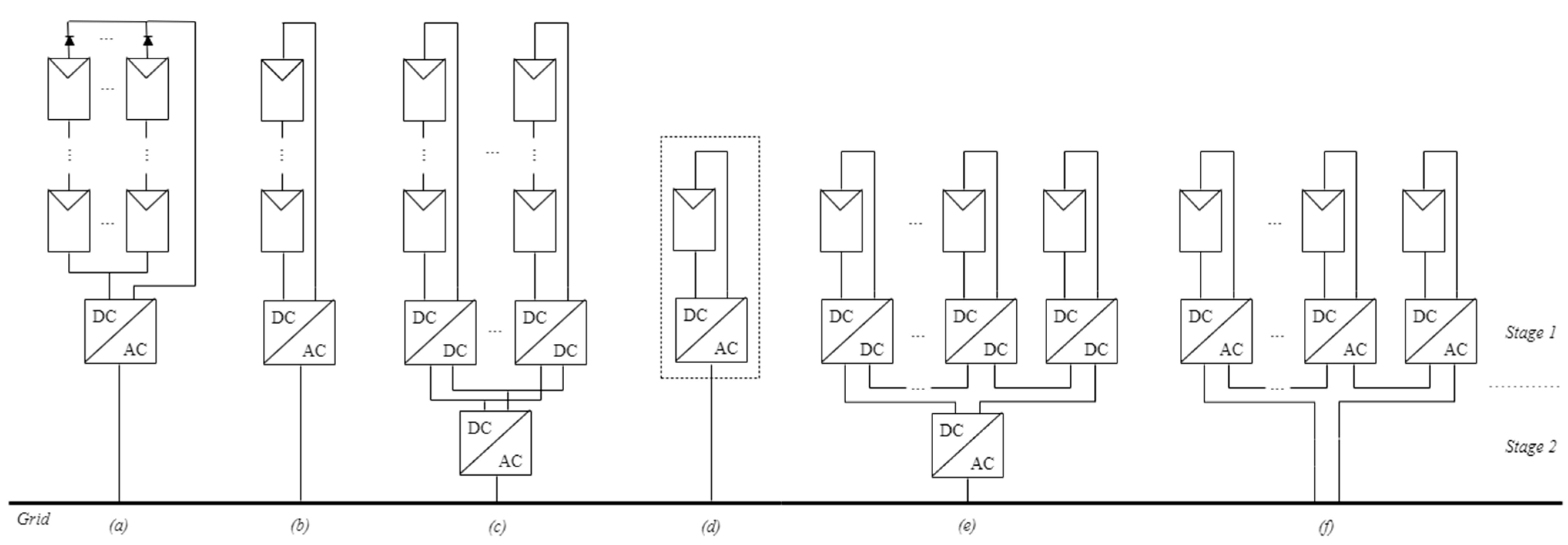
2.3. Arrangements for Power Transfer

The centralized converters (Figure 1a) are characterized by the interconnection of all photovoltaic modules into a single inverter. In this configuration, the photovoltaic panels are interconnected in series, resulting in a voltage high enough that no further power conversion stage is needed. To increase the electric power generated, more branches of panels can be inserted in parallel, provided that due care be taken against reverse currents that may arise if one of the strings is shaded. Common ways to protect shaded strings from reverse currents are fuses or diodes in series. Centralized converters were the first to be used, however, disadvantages such as high DC voltage, difficulty in tracking maximum power in shading situations and losses in series diodes motivated the search for alternatives to overcome such difficulties [12,15].

A way to improve the efficiency in applications with centralized converters is the use of only one string of PV modules. This configuration is known as a string converter (Figure 1b) and it allows a better use of electrical energy supplied by the set of panels. In this case, there are no conduction losses from the series diodes since they become unnecessary. Thus, likewise the case with centralized inverters, power switches are needed to support the open circuit voltage of the entire string.

In order to increase the power generation without losing the string converter benefits and minimizing the PS effects, the multi-strings converter emerges as a good alternative (Figure 1c). In this topology, each branch has a DC-DC converter to carry out its respective MPPT. Such a strategy considerably improves the efficiency of tracking the global MPP. There is a common DC bus to parallel the DC-DC converters output, followed by the inverter module that controls the current transferred to the power grid.

Figure 1d shows a representation of the AC module. This setting, commonly known as a microinverter, allows a panel (or an arrangement with few panels) to be connected to the grid. In this case, each panel will have its own MPPT algorithm, which guarantees the optimized operation in terms of power tracking. Since it is a topology that needs to be replicated to increase the injected power, it becomes more costly as compared to the centralized structures. On the other hand, it is a versatile proposal, which allows planned expansion of the system, greater reliability, maintenance without interruption of operation, and optimized adjustment of the injected power. Its cost has been reduced with the manufacture in scale [16].

Another possibility is the use of cascade DC-DC converters, as seen in Figure 1e. In this configuration, each DC-DC converter controls the MPPT of a panel (or a small PV arrangement) and associates them in series. A controlled DC bus, with voltage enough to supply the DC-AC inverter, is created. This configuration becomes less expensive when compared to the AC module (Figure 1d), since it uses a single DC-AC stage. However, it does not have the same versatility to increase or reduce the injected power.

A second possibility of using cascade converters is presented in Figure 1f. In contrast with the previous ones, the DC-AC cascade inverter uses only one stage of power conversion. Each PV module is connected to a DC-AC converter whose output is in series with the output of the other converters. Such a configuration has the good feature of being similar to the AC module converter, bringing a better use per PV module due to the individual MPPT, however, with lower cost and greater efficiency [12].

From the knowledge of the main advantages and disadvantages of each grid connection architecture, it is observed that multilevel topologies can be better explored mainly because they are a good option in PS situations. They are also interesting for operating with lower switching frequencies, for having better performance when dispensing the DC-DC boost stage, and for not having high voltage DC buses [12,15].

In view of good stability during grid-tied operation, many control techniques are presented throughout literature review. An attractive solution with relative simplicity of implementation is the virtual synchronous generator (VSG), including for a cascaded H-bridge multilevel PV converter [17]. However, facing PS situations, its poor dynamic response results in sudden voltage oscillations and imposes the use of battery banks or reserve PV modules to operate as a power buffer.

Among the topologies used for PS solution, this work chose the cascaded multilevel converter as the stage of energy conversion. It allowed for the performance of the MPPT individually or with a small PV array, making it possible to use a classic MPPT algorithm. The control philosophy for power transfer were based on the fundamentals of a VSG, however, without using any power buffer. Compared to [12], the VSG is simpler since there is no need to tune controllers. The droop dynamics is slow, which suggests the need for a power buffer as in [17]. However, this work proposes a differentiated control to regulate the output voltage of the converter. The idea is to use two control loops that update both the power reference to be transmitted and the energy distribution delivered by each PV array.

3. System Overview

3.1. Multilevel Topology

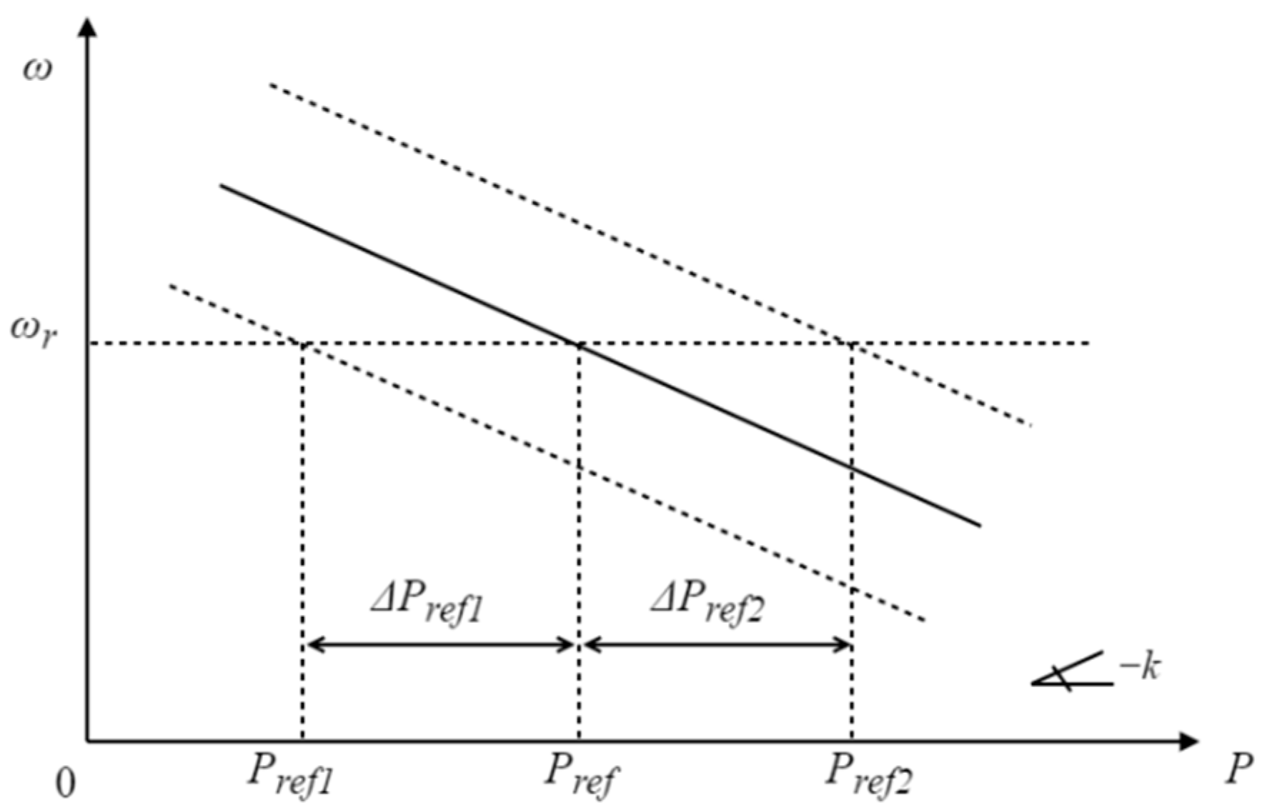
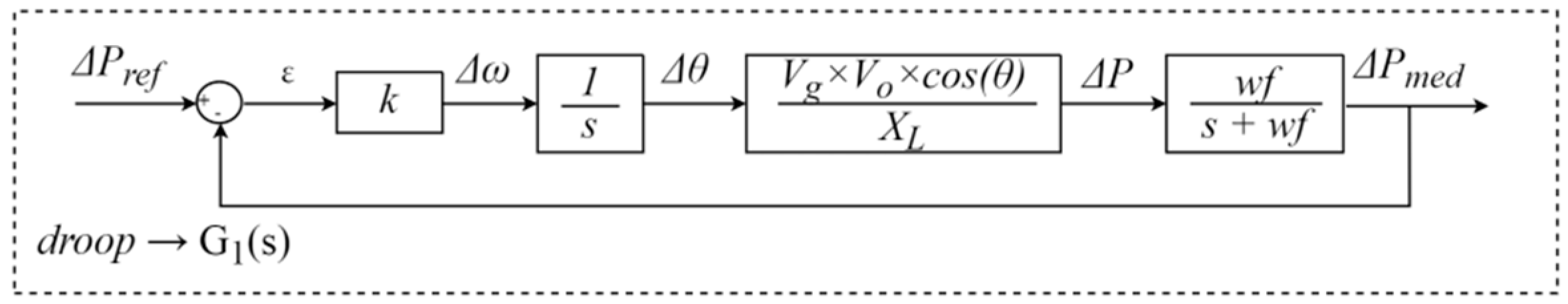
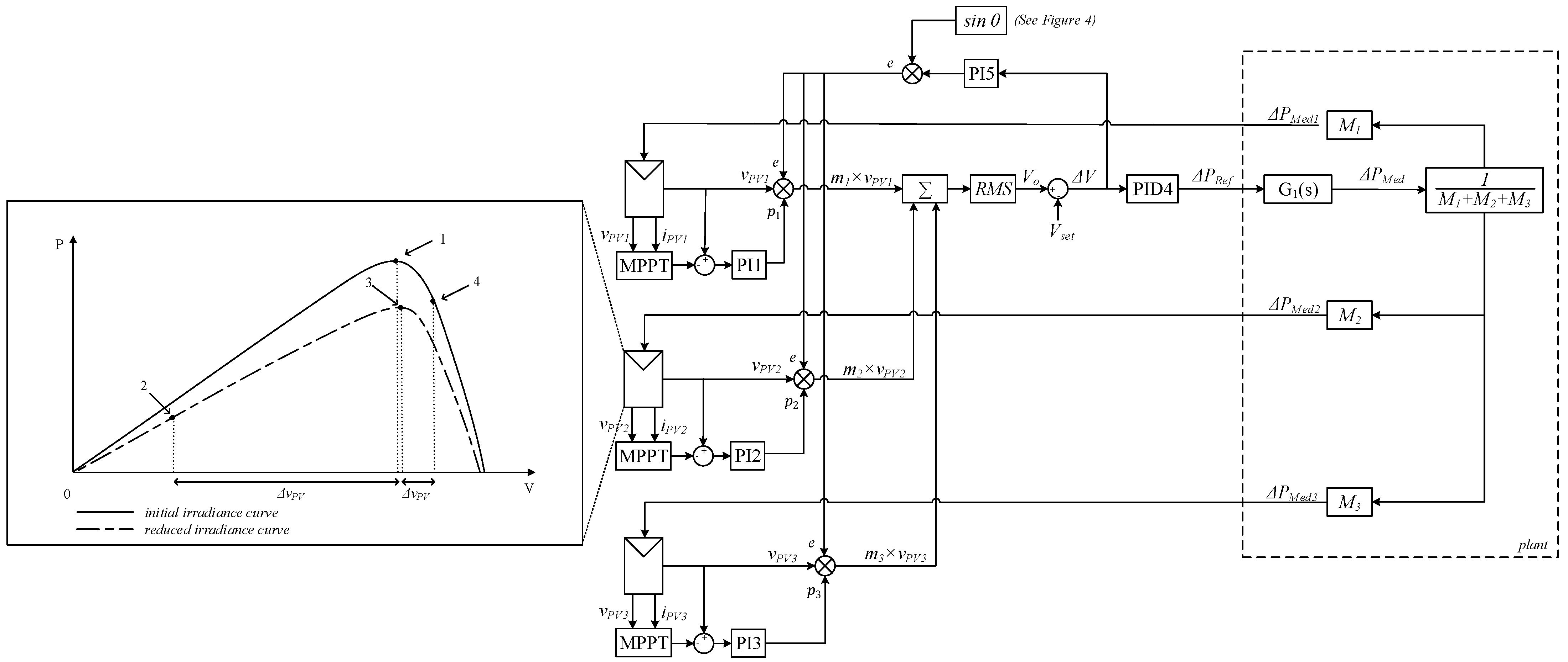
To achieve the maximum power transfer in PS situations, it is assumed that the MPPT is carried out in each PV module or in a set of a few modules, which allows the use of classical MPPT techniques. The MPPT used in this work was the perturb and observe (P&O) [2,18], however, it could be any other classic technique. Therefore, in order to deal with PS conditions and providing other advantages such as low complexity and high performance, a seven-level Cascaded H-Bridge Inverter (CHB-ML) was chosen, as shown in Figure 2.

Regarding the use of multilevel inverters, there are always additional concern with the modulation techniques, as each level must respect a switching logic to obtain the desired output voltage. For this purpose, to facilitate the distribution of power to the different levels, phase shifted pulse width modulation (PS-PWM) was used. PS-PWM is the most popular carrier-based modulation technique due to its advantages in power balancing, good output harmonics and simplicity of implementation [19,20]. Much has been studied to improve its performance, especially to reduce the switching frequency, however, increasing the complexity [21,22].

With the proposed multilevel topology, the increase in the number of levels depends on the increase in cascade inverter modules (n). Consequently, aiming to guarantee an output voltage based on the modulation signal waveform, each new inverter module will have its switching logic from pulses generated by a new carrier signal. As shown in (1), for the PS-PWM the carrier signals must respect a uniform phase shift (δ) between them:

$$\delta =180°/n.$$

(1)

3.2. VSG Control

In an electric power system, the active power flow $\left(P\right)$ can be calculated using (2), where $V_o$ and $V_g$ are the inverter output voltage and the mains voltage, respectively. In (2), $\theta$ corresponds to the power angle obtained from the angular difference between such voltages, and the resistance $\left(R\right)$ and inductive reactance $(X_L)$ make up the connection impedance.

$$P=\frac{R\times V_o{}^2-R\times V_g\times V_o\times \cos \left(\theta \right)+X_L\times V_g\times V_o\times \sin \left(\theta \right)}{R^2+X_L{}^2}$$

(2)

For situations in which the connection impedance is predominantly inductive, the variation in the transmitted power in relation to the power angle $\left(\frac{\delta P}{\delta \theta }\right)$ can be linearized to an operating point as seen in (3).

$$\Delta P=\frac{V_g\times V_o\times \cos \left(\theta \right)}{X_L}\times \Delta \theta$$

(3)

As noted in (3), $\theta$ was chosen to control the transmitted power. The practical and robust way to change $\theta$ is to act in the converter angular frequency $\left({\omega }_r\right)$. A very useful technique to update ${\omega }_o$ mimics the synchronous generator and it is called droop-control. In addition to the simplicity of its implementation, this controller guarantees intrinsic stability for on-grid operation and eliminates the necessity of intercommunication loops between generators. In (4), the rule that governs the droop-control is presented. In addition to ${\omega }_o$, the variables present in (4) are the grid angular frequency $({\omega }_r$), the power to be transmitted $\left(P_{ref}\right)$, the power delivered by the converter $(P_{med})$, and the coefficient $k$ which defines the slope of the droop-control curve [23].

$${\omega }_o={\omega }_r+k\left(P_{ref}-P_{med}\right)$$

(4)

Assuming a generator set already connected to the power grid, from the change of $P_{ref}$ the $P-\omega$ curve will be adjusted to change the transmitted power. In this way, a new equilibrium point will be reached since the system will balance in ${\omega }_r$. According to Figure 3, dashed lines represent slope curves for situations whose reference power has changed.

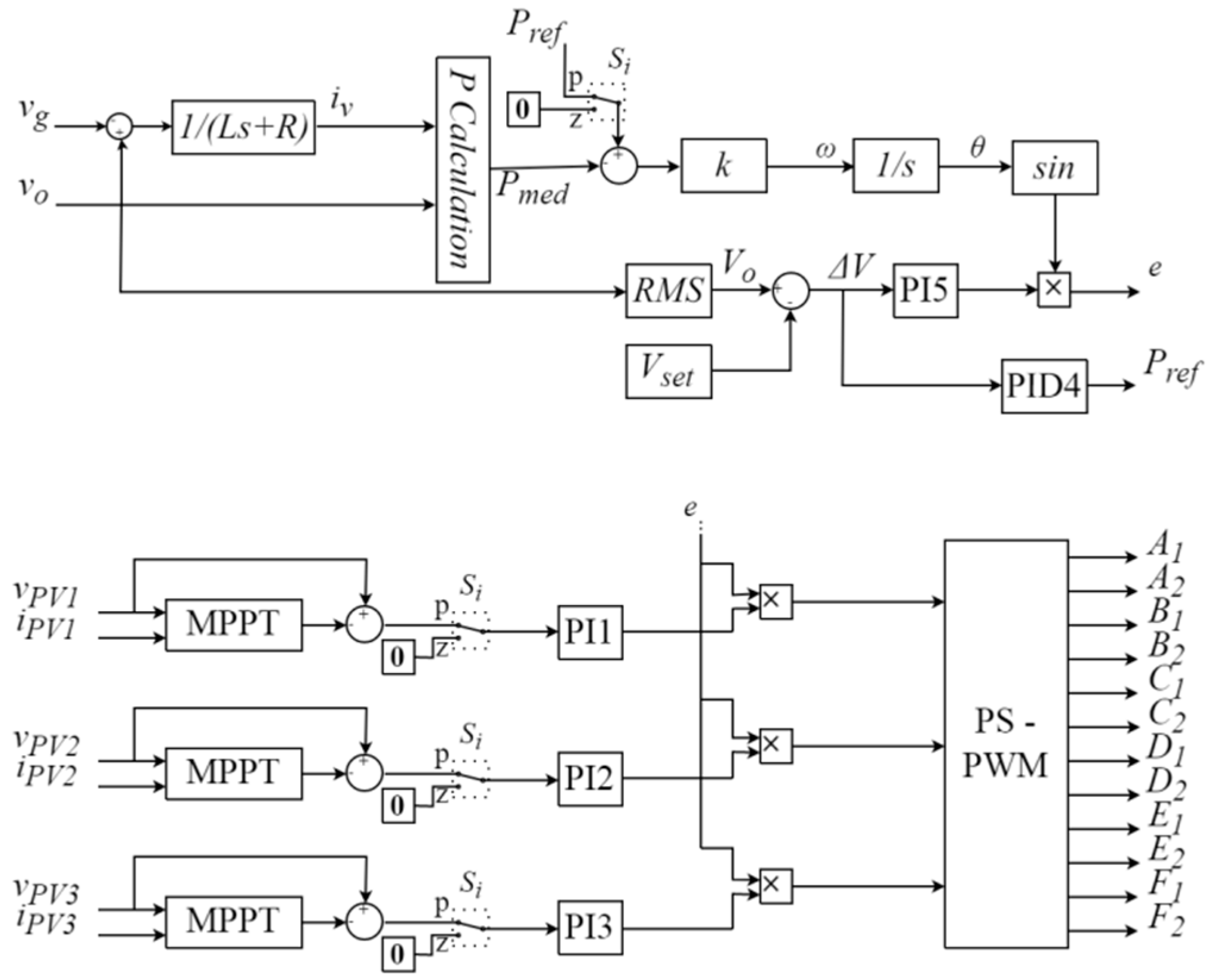
3.3. Control Philosophy

The block diagram that describes the dynamic behavior of a droop-controller is represented in Figure 4. The control action occurs from perturbations in $P_{med}$ and $P_{ref}$. According to the droop-control slope (k), the power error (ε) results in variations in the system frequency $\left(\Delta \omega \right)$. Consequently, the power angle $\left(\theta \right)$ is perturbed and the output power is also modified. The power calculation is processed through the instantaneous product between the real output voltage $(v_o)$ and the virtual current $(i_v)$. The presence of the low-pass filter is necessary to obtain the average value of the instantaneous output power [24]. In Figure 5, the low-pass filter is inserted in the block called PCalculation.

As noted, the droop-control imposes a slow dynamic by acting on average power values. Furthermore, the system plant cannot collaborate for fast controller actions due to the connection reactance. Such characteristics impose an additional challenge to the transfer of power in situations of PS or sudden variations in irradiation. The controller needs to be tuned so that the power transferred to the grid occurs with a relatively quick response as the irradiation variations occur. If this dynamic response is not appropriate, the voltages in the panels can suffer sudden variations and consequently impact the connection voltage. An intermediate stage, between panels and the H-bridge inverter, could facilitate the dynamics, for it would serve as a supplier or accumulator of energy in the respective situations from a transient to a low or high irradiance. However, aiming to lower cost and better performance, this paper proposes the use of a single-stage converter.

The solution found to minimize the effects of rapid variations in irradiance was to use the output voltage as the main power transfer control variable. To this end, it is necessary to have a controller fast enough to sustain the connection without the PV sets suffering irreversible voltage sags due to the sudden reductions in irradiation. Another challenge is to have a controller with proper tuning to ensure the connection without overloading the system when there is a rapid rise of irradiation. To solve such adversities, the controller presented in Figure 5 is proposed.

According to diagrams in Figure 5, the control system uses the reading of eight variables, being: PV arrays voltages (v_PV1, v_PV2 e v_PV3), PV arrays currents (i_PV1, i_PV2 e i_PV3), grid voltage (v_g), and multilevel inverter output voltage (v_o). In accordance with (5), the converter output current (i_v) is calculated through a virtual impedance, where R and L correspond to the approximated values of the connection resistance and inductance, respectively.

$$i_v\left(s\right)=\frac{v_r\left(s\right)-v_o\left(s\right)}{Ls+R}$$

(5)

In Figure 5 are presented the blocks that make up the droop controller. When the switch S is in the “z” position, the controller causes $P_{med}$ to be zero, resulting in synchronism with the grid. When the switch S is in the position “p”, the converter tracks the power $P_{ref}$. To preserve the connection stability, before the action of the power tracking algorithms (PI1, PI2 and PI3), the PID4 controller acts based on the error between the inverter RMS output voltage ($V_o$) and the reference voltage ($V_{set})$. Thus, before any tracking, the droop control acts on the power angle to reduce or increase power transfer and to preserve both PV and output inverter voltages. In parallel to PID4, the controller called PI5, also in anticipation of the tracking controllers, acts to regulate the amplitude of the signal (e) that modulates the output voltage and that ends up controlling the reactive power flow. However, mainly for low irradiation situations, some content of reactive power may be present in the system, after all these situations are more complex to regulate $V_o$. Although in this work the reactive power control was not addressed, an effective way to overcome this drawback depends on an additional controller and measurements or estimations of the reactive power. Thus, $V_{set}$ and $\theta$ could be updated to minimize or cease the reactive power. Another point to be highlighted refers to the limit of voltage regulation imposed by the PV arrays. There is no link DC for voltage regulation, which means that, depending on the level of solar irradiation, the presence of reactive power becomes unavoidable, forcing the system disconnection if any amount of reactive power can be tolerated.

Now, by observing the diagram in Figure 5, from a new irradiation condition, controllers PI1, PI2 and PI3 act in the power tracking through the duty cycle of each inverter block. In this way, the indexes m_i are adjusted in proportion to the amount of power that each inverter module will process. Since the MPPT acts on the modulation indexes, this action results in the variation of the output voltage, instructing the PID4 controller to vary $P_{ref}$ for the new power situation while PI5 adjusts the amplitude $\left(e\right)$ to prevent reactive flow.

The controller gains are shown in

Table 1. Controllers’ gains.

	kp	ki	kd
PI 1, 2, 3, 5	0.001	0.01	0
PID 4	15	20	0.1

. Due to the non-linear characteristic of the photovoltaic panels, there was some difficulty in modeling the plant response, leading, a priori, to select the gains based on simulations.

3.4. Effects of Irradiation Variations

Figure 6 presents the complete view of the system. An important point to observe in this representation refers to the PV arrays voltages. These voltages depend on the solar irradiation, and they are also affected by the delivered power variation. Consequently, PV voltage variations strongly interfere in the inverter output voltage, which makes its regulation a challenging task. It is also important to mention that the part surrounded by the dashed lines concerns the droop-control and the physical plant operation $\left(G_1\right)$. $\Delta P_{medi}$ represent the powers delivered by each inverter bridge. Note that these powers are the result of the tracked power weighted by the modulation indexes $(M_i)$, in this case represented by the RMS values of $m_i$. Looking at Figure 5 and Figure 6, it is noteworthy that $m_i$ are obtained from the product between two signals, which means, they depend on both the MPP tracking $\left(p\right)$ and the modulating $\left(e\right)$ updating.

Analyzing the curve zoomed in Figure 6, it is concluded that the main dynamic difficulty occurs with the sudden reduction of irradiation. Suppose that a given PV set is at the point of operation identified on the curve as “1”. With the reduction of irradiation, the power transferred to the grid does not change instantly, requiring more power than that available on the panels at that time. As shown at point “2”, this situation causes the collapse of the panel voltage and, consequently, the converter output voltage. From the PID4 controller action, the power transfer is reduced, and the voltage of the panels is restored until the plant is driven to the new MPP, represented by the point “3”. If there is a return to the original irradiation, there will be an instantaneous increase in the PV voltages and available power, which will cause the system to operate momentarily at point 4. Finally, with the action of the MPPT algorithm and the other controllers, the system will be taken to the original operating point, identified in the curve by “1”.

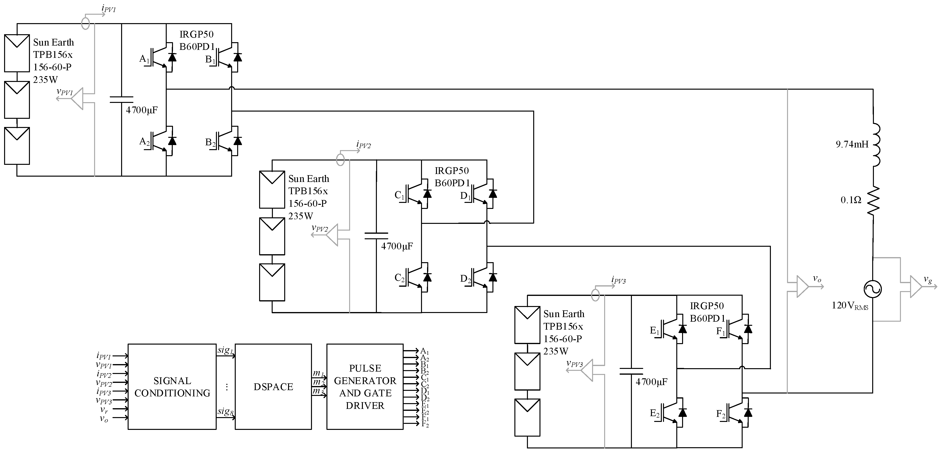
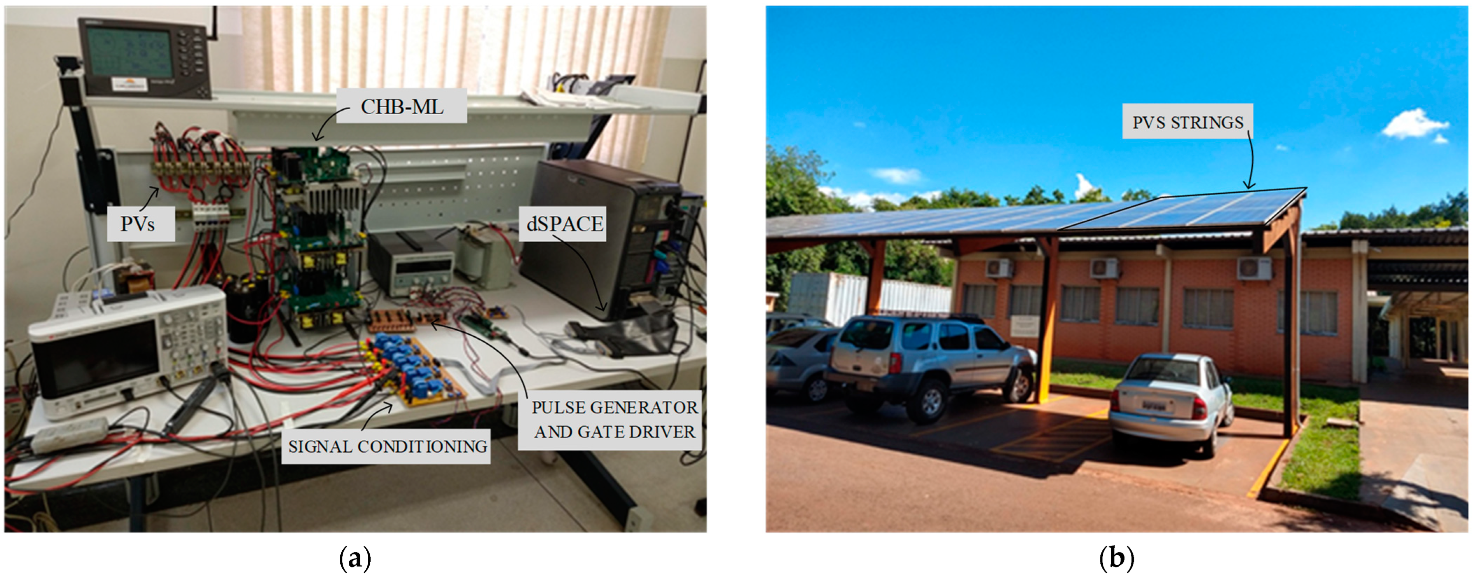
4. Experimental Evaluation

4.1. System Overview

Figure 7 contains a general schematic and

Table 2. System and PV panel electrical parameters.

Parameters	Values
DC-link capacitor	4700 µF
Connection inductance	9.74 mH
Connection resistance	0.1 Ω
Switching frequency	2.5 kHz
Mains frequency	60 Hz
Rated grid voltage	120 VRMS
Maximum power PV	235 Wp
Voltage at MPP	29.2 V
Current at MPP	7.6 A
Open circuit voltage	32.9 V
Short circuit current	7.6 A

summarizes the electric parameters for the circuits used for grid connection. As noted, each inverter bridge works from a PV array formed by three photovoltaic panels in series. For the experiments, a real plant was used, composed of Sun Earth^® panels, model TBP156 × 156-60P, with rated power of 235 W. In the input of each inverter bridge, an electrolytic capacitor of 4700 µF was used to minimize the inductive effect of connection cables between panels and inverters. To compose the H-bridge, since it is a prototype whose controllers would need experimental adjustments, it was decided to use power switches with over-rated characteristics, ensuring robustness even in adverse operating conditions. The switch model adopted was the IRGP50B60PD1, with blocking voltage of 600 V and continuous operating current of 33 A. For connection to the mains, a 9.74 mH connection inductor with an intrinsic resistance of about 100 mΩ was used.

The control system consists essentially of the three blocks shown in Figure 7. At first, the sampled signals go through the conditioning hardware to adjust amplitudes and filter noise. The conditioned signals (sig₁, ..., sig₈) go to the control system embedded in the DSPACE^® processor. As a result of the control actions, the modulating signals (m₁, m₂ and m₃) go to an external hardware where they are compared to the triangular carriers to generate the switching pulses. Figure 8a,b show, respectively, the implemented prototype and the set of photovoltaic panels used during the experiments.

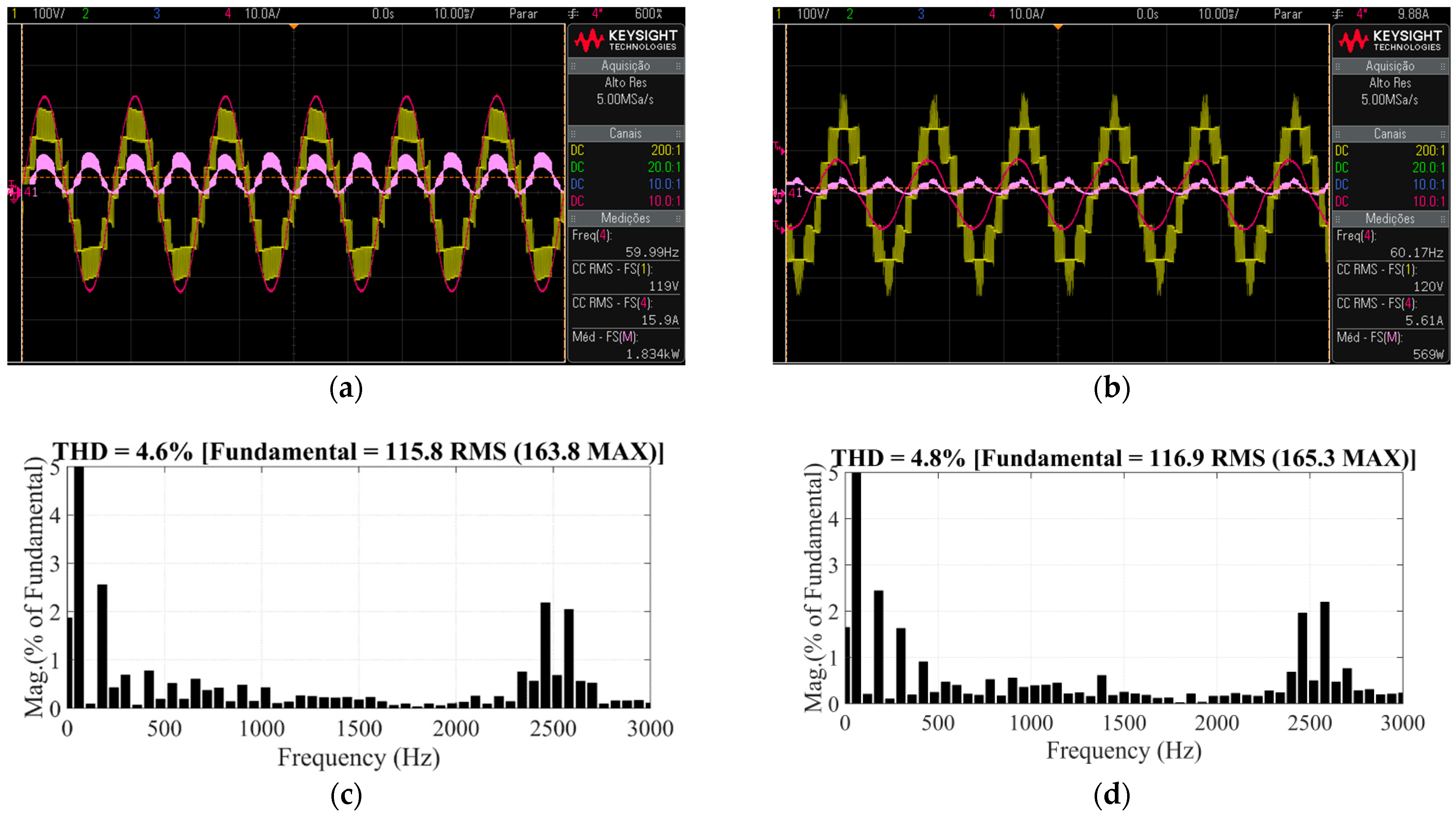
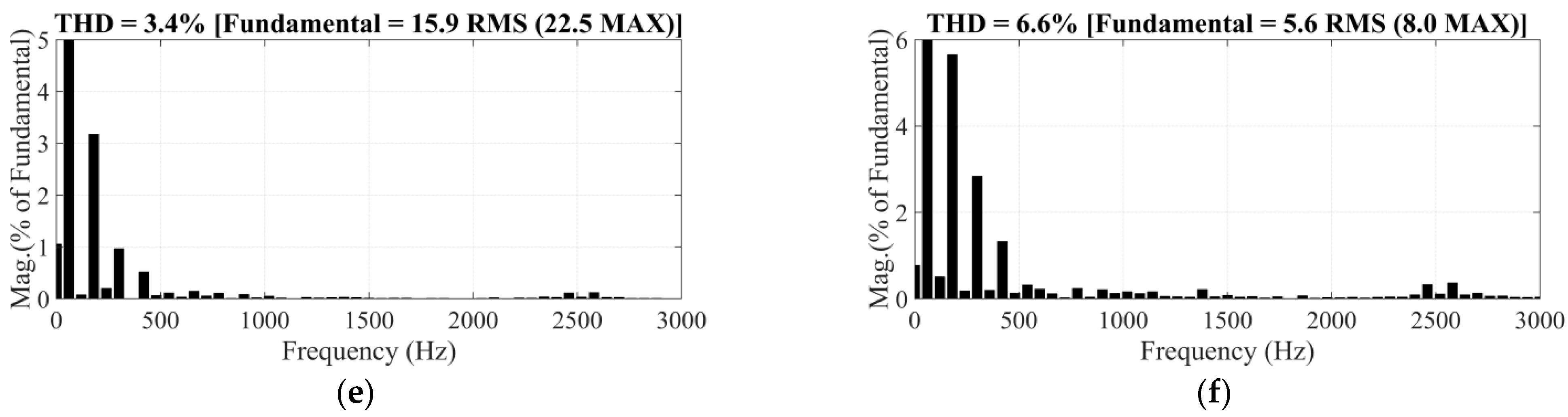
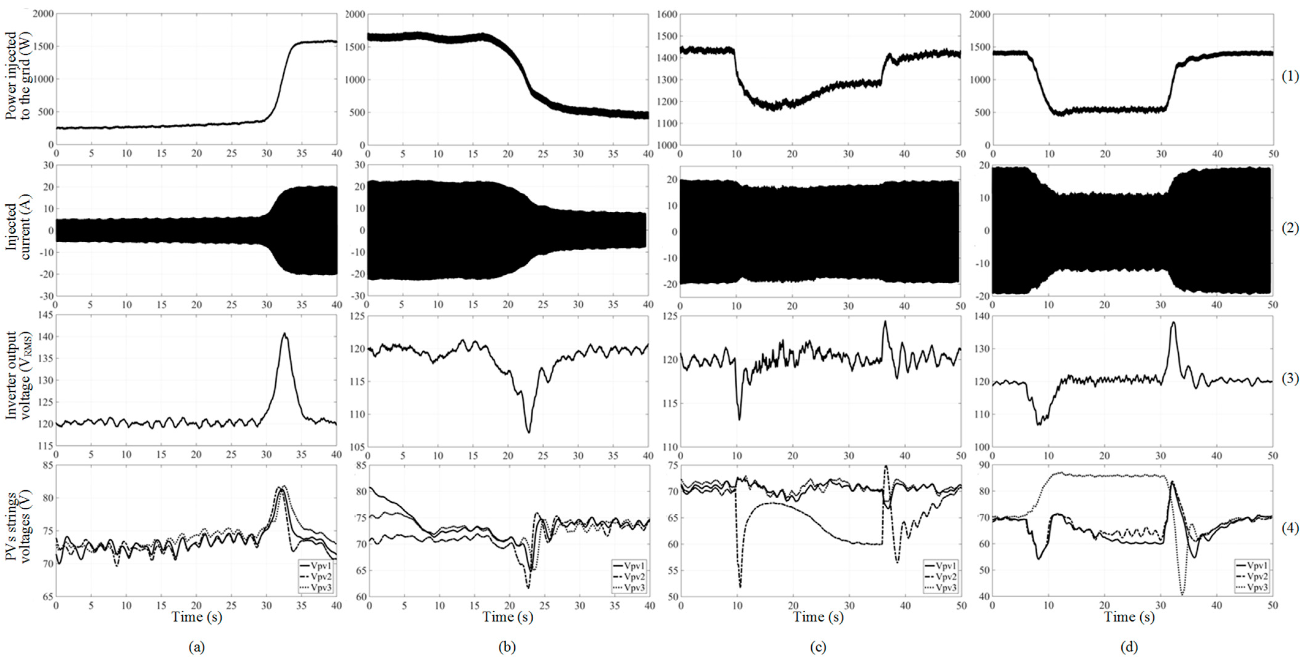
4.2. Experimental Results

Figure 9a contains the waveforms for the CHB-ML output voltage (yellow), current (red) and power (magenta) injected into the electrical grid during irradiation of 1250 W/m². Still for this situation, the inverter voltage and current harmonic spectra are shown in Figure 9c,e, respectively. Figure 9b contains the waveforms for the voltage (yellow), current (red) and power (magenta) during irradiation of 300 W/m². The harmonic spectra for both the inverter voltage and output current are shown in Figure 9d,f, respectively. For all situations, THD was calculated considering harmonics up to 3 kHz. The electrical parameters for the situations of high and low irradiance are summarized in

Table 3. Comparison between steady-state parameters for high and low irradiance.

	1250 W/m2	300 W/m2
PVs Temp	~60 °C	~45 °C
VPV1	71.5 V	82.5 V
VPV2	71.0 V	82.8 V
VPV3	70.9 V	83.3 V
IPV1	9.4 A	2.6 A
IPV2	9.7 A	2.6 A
IPV3	9.5 A	2.4 A
VO	119 VRMS	120 VRMS
IO	15.9 ARMS	5.6 ARMS
PO	1834 W	569 W
m1	0.79	0.68
m2	0.86	0.72
m3	0.84	0.68

. It is interesting to observe the equilibrium reached by the indexes $m_i$ denoting the small differences in the power contribution of each PV array for both situations. Another point to be considered is the superiority of the indexes for high irradiation, confirming the more significant contribution of the PV arrays for this condition.

An important characteristic of PS-PWM is the capability of dealing with different indexes m_i in each inverter while maintaining an output voltage waveform with low THD. However, in situations where the contribution of one (or more) of the PV arrays is very low, the controller can lead its respective modulation index m_i to smaller values, reducing the respective inverter contribution. For these situations, if the output voltage cannot be reached or if the current THD becomes poor, the system must be disconnected.

Aiming to evaluate the currents THD for the results presented in Figure 9, some considerations are noteworthy. First, this application consists of a reduced number of levels, which harden the current and voltage quality in some situations. The presence of DC level and third harmonic in the currents are slightly superior to the limits recommended by the IEEE Standard 1547-2018. Another important point refers to the absence of any high-frequency filter, resulting in the converter output voltage with significant high-order content. Based on the preliminary results, although some efforts must be concentrated to improve the quality of the voltage and current waveforms, it is reasonable to conclude that the ML-CHB and PS-PWM are a promising choice for PS conditions, especially for situations with a greater number of levels, where voltage regulation and THD will be appreciably improved.

Figure 10 shows the behavior of the system under different situations of irradiation and PS. In the scenario presented in Figure 10a, graphic 1 represents the power transferred to the electrical grid. According to the voltage curves of the photovoltaic arrays, shown in graphic 4, the increase in irradiance raises the voltage in the PV sets. As a matter of consequence, there is an increase in the output voltage of the inverter (graphic 3), which determines the essential need for increasing power transfer. Therefore, the output voltage stabilizes as the new MPPT is reached. Both in graphic 1, referring to the power transferred to the power grid, and in graphic 2, referring to the current injected into the power grid, it is evident that the system stabilizes at a new point of operation after the increase in irradiance.

Figure 10b contains the curves corresponding to the situation of sudden irradiance reduction. Similar to the previous case, the PV sets voltage variation is reflected to the output voltage (graphic 3). Since the available power has been reduced and the transferred power is still the same, the tendency is to bring the panels to extremely low voltage levels that can be irreversible and can cause the power transfer to be definitively interrupted. Therefore, it is necessary for the control system to act from the output voltage sag, reducing the transferred power as quickly as possible until the tracking of the new MPP is achieved.

The situation presented by the graphs in Figure 10c corresponds to the shading of one PV array. As shown in graphic 1, referring to the power injected to the mains, shading occurs from the time of 10 s to the time of 36 s. According to the PV sets voltage curves (graph 4), promptly after shading, the control acts to reduce the transferred power to relieve the drained power and to recover the voltage of the shaded array. Still with a view at the curves referring to the behavior of the PV array voltages, it is noted that the tracking of the new MPP is established around the instant of 30 s. After the shading being removed, around 36 s, the control system acts to stabilize the rise in the output voltage and to track the new MPP.

Figure 10d presents a very peculiar operation scenario. In this condition, from the instant of 7 s, two PV arrangements were completely shaded, leaving only one arrangement exposed to sunlight. The shading lasted until approximately 31 s. It is worth mentioning that this condition did not allow the system to operate in its new MPP. If the new MPP were tracked, there would not be enough voltage on the panels to guarantee the regulation of the inverter output voltage at 120 V_RMS. Therefore, due to the reduction in the voltage of the PV arrays (graphic 4), there is an abrupt reduction in the inverter output voltage (graphic 3), which leads to the immediate need of decreasing the power transferred to the grid. As the transferred power decreases, the voltage of the arrays is restored and, consequently, the output voltage of the inverter is regulated again. However, based on the curves shown in graphic 4, once the output voltage regulation has been prioritized (graphic 3), the arrangement without shading is prevented from operating at its maximum power point. After the shading is removed, the output voltage is momentarily increased, and the maximum power point tracking is achieved. The curves corresponding to the transferred power (graphic 1) and the current injected into the grid (graphic 2) make the operating points noticeably clear before, during and after the two PV sets are shaded.

5. Conclusions

In accordance with the results achieved, the ML-CHB topology is presented as a good solution for dealing with the problem PS. Current research as well as market demands make evident the need for structures with better performance and addition of MPPT algorithms for a PV plant. In addition to ensuring a low THD output voltage, the CHB-ML is a single stage structure which allows the use of an MPPT algorithm for each power module. The number of levels can be set based on the need for the project, considering the output voltage and the number of tracking algorithms intended to be implemented. Simplification of control strategies becomes a relevant approach for the use of CHB-ML topology, and the use of the VSG control demonstrated robustness, ease of implementation and possibility of operation for islanding situations. Of course, the results show that the dynamic response of the droop control is truly slow. However, it is emphasized that in practical situations an extremely fast dynamic response is not required, since the irradiance variations during PS are not as sudden as those assessed in this paper. An important feature of the proposed control is the possibility of power tracking in two stages. Firstly, there is the prompt action of PID4 controller to adjust the power transfer based on the oscillations of the converter output voltage. Subsequently, the remaining controllers act to ensure the fine adjustment for tracking the MPP and to regulate the output voltage. It is reasonable to mention that, from plant adaptations, i.e., the reduction of the current connection impedance, the controllers can be tuned for a better dynamic response. Currently, the authors have studied the alternative of replacing the PID4 controller with a fuzzy-logic controller. This approach intends to improve the system stability and to ensure specific responses for situations of PS with sudden irradiance variations. Furthermore, it must be mentioned that the individual or global tracking factors were not evaluated, for infrastructure limitations made it difficult the achievement of V-I curves of the real PV arrays. Although the development was focused on keeping the system stability in sudden PS transitions, it was confirmed significant coherence among the delivered power for different irradiations. For future works, the authors intend not only to evaluate the PVs tracking factors but also to increase the number of levels, which will result in better output voltage quality and regulation, in addition to one MPPT per panel.

References

1. Zhang, P.; Sui, H. Maximum Power Point Tracking Technology of Photovoltaic Array under Partial Shading Based On Adaptive Improved Differential Evolution Algorithm. Energies 2020, 13, 1254. [Google Scholar] [CrossRef]
2. De Brito, M.A.G.; Galotto, L.; Sampaio, L.P.; Melo, G.D.A.E.; Canesin, C.A. Evaluation of the Main MPPT Techniques for Photovoltaic Applications. IEEE Trans. Ind. Electron. 2013, 60, 1156–1167. [Google Scholar] [CrossRef]
3. Villalva, M.G.; Gazoli, J.R.; Filho, E.R. Comprehensive Approach to Modeling and Simulation of Photovoltaic Arrays. IEEE Trans. Power Electron. 2009, 24, 1198–1208. [Google Scholar] [CrossRef]
4. Bollipo, R.B.; Mikkili, S.; Bonthagorla, P.K. Hybrid, optimal, intelligent and classical PV MPPT techniques: A review. CSEE J. Power Energy Syst. 2021, 7, 9–33. [Google Scholar] [CrossRef]
5. Eltamaly, A.M. An Improved Cuckoo Search Algorithm for Maximum Power Point Tracking of Photovoltaic Systems under Partial Shading Conditions. Energies 2021, 14, 953. [Google Scholar] [CrossRef]
6. Barcellona, S.; Barresi, M.; Piegari, L. MMC-Based PV Single-Phase System with Distributed MPPT. Energies 2020, 13, 3964. [Google Scholar] [CrossRef]
7. Alves, T.; Torres, J.P.N.; Marques Lameirinhas, R.A.; Fernandes, C.A.F. Different Techniques to Mitigate Partial Shading in Photovoltaic Panels. Energies 2021, 14, 3863. [Google Scholar] [CrossRef]
8. Kim, K.A.; Seo, G.-S.; Cho, B.-H.; Krein, P.T. Photovoltaic Hot-Spot Detection for Solar Panel Substrings Using AC Parameter Characterization. IEEE Trans. Power Electron. 2016, 31, 1121–1130. [Google Scholar] [CrossRef]
9. Rossi, D.; Omaña, M.; Giaffreda, D.; Metra, C. Modeling and Detection of Hotspot in Shaded Photovoltaic Cells. IEEE Trans. Very Large Scale Integr. Syst. 2015, 23, 1031–1039. [Google Scholar] [CrossRef]
10. Batzelis, E.I.; Georgilakis, P.S.; Papathanassiou, S.A. Energy models for photovoltaic systems under partial shading conditions: A comprehensive review. IET Renew. Power Gener. 2015, 9, 340–349. [Google Scholar] [CrossRef]
11. Engel, E.; Kovalev, I.; Testoyedov, N.; Engel, N.E. Intelligent Reconfigurable Photovoltaic System. Energies 2021, 14, 7969. [Google Scholar] [CrossRef]
12. Xiao, B.; Hang, L.; Mei, J.; Riley, C.; Tolbert, L.M.; Ozpineci, B. Modular Cascaded H-Bridge Multilevel PV Inverter with Distributed MPPT for Grid-Connected Applications. IEEE Trans. Ind. Appl. 2015, 51, 1722–1731. [Google Scholar] [CrossRef]
13. Chavan, V.C.; Mikkili, S.; Senjyu, T. Hardware Implementation of Novel Shade Dispersion PV Reconfiguration Technique to Enhance Maximum Power under Partial Shading Conditions. Energies 2022, 15, 3515. [Google Scholar] [CrossRef]
14. Vadivel, S.; Boopthi, C.S.; Ramasamy, S.; Ahsan, M.; Haider, J.; Rodrigues, E.M.G. Performance Enhancement of a Partially Shaded Photovoltaic Array by Optimal Reconfiguration and Current Injection Schemes. Energies 2021, 14, 6332. [Google Scholar] [CrossRef]
15. Kjaer, S.B.; Pedersen, J.K.; Blaabjerg, F. A review of single-phase grid-connected inverters for photovoltaic modules. IEEE Trans. Ind. Appl. 2005, 41, 1292–1306. [Google Scholar] [CrossRef]
16. Alluhaybi, K.; Batarseh, I.; Hu, H. Comprehensive Review and Comparison of Single-Phase Grid-Tied Photovoltaic Microinverters. IEEE J. Emerg. Sel. Top. Power Electron. 2020, 8, 1310–1329. [Google Scholar] [CrossRef]
17. Zhang, X.; Hu, Y.; Mao, W.; Zhao, T.; Wang, M.; Liu, F.; Cao, R. A Grid-Supporting Strategy for Cascaded H-Bridge PV Converter Using VSG Algorithm with Modular Active Power Reserve. IEEE Trans. Ind. Electron. 2021, 68, 186–197. [Google Scholar] [CrossRef]
18. Mohamed Hariri, M.H.; Mat Desa, M.K.; Masri, S.; Mohd Zainuri, M.A.A. Grid-Connected PV Generation System—Components and Challenges: A Review. Energies 2020, 13, 4279. [Google Scholar] [CrossRef]
19. Sochor, P.; Akagi, H. Theoretical and Experimental Comparison between PhaseShifted PWM and Level-Shifted PWM in a Modular Multilevel SDBC Inverter for Utility-Scale Photovoltaic Applications. IEEE Trans. Ind. Appl. 2017, 53, 4695–4707. [Google Scholar] [CrossRef]
20. Akhmetov, Z.; Hammami, M.; Grandi, G.; Ruderman, A. On PWM Strategies and Current THD for Single- and Three-Phase Cascade H-Bridge Inverters with Non-Equal DC Sources. Energies 2019, 12, 441. [Google Scholar] [CrossRef] [Green Version]
21. Kim, S.-M.; Lee, E.-J.; Lee, J.-S.; Lee, K.-B. An Improved Phase-Shifted DPWM Method for Reducing Switching Loss and Thermal Balancing in Cascaded H-Bridge Multilevel Inverter. IEEE Access 2020, 8, 187072–187083. [Google Scholar] [CrossRef]
22. Guo, X.; Wang, X.; Wang, C.; Lu, Z.; Hua, C.; Blaabjerg, F. Improved Modulation Strategy for Singe-Phase Cascaded H-Bridge Multilevel Inverter. IEEE Trans. Power Electron. 2022, 37, 2470–2474. [Google Scholar] [CrossRef]
23. Godoy, R.B.; Bizarro, D.; De Andrade, E.T.; Soares, J.D.O.; Ribeiro, P.E.M.J.; Carniato, L.A.; Kimpara, M.L.M.; Pinto, J.O.P.; Al-Haddad, K.; Canesin, C.A. Procedure to Match the Dynamic Response of MPPT and Droop-Controlled Microinverters. IEEE Trans. Ind. Appl. 2017, 53, 2358–2368. [Google Scholar] [CrossRef]
24. Godoy, R.B.; Pinto, J.O.P.; Canesin, C.A.; Coelho, E.A.A.; Pinto, A.M.A.C. Differential-Evolution-Based Optimization of the Dynamic Response for Parallel Operation of Inverters with No Controller Interconnection. IEEE Trans. Ind. Electron. 2012, 59, 2859–2866. [Google Scholar] [CrossRef]
Figure 1. Power plants for grid connection: (a) central inverter; (b) string inverter; (c) multistring inverter; (d) ac-module inverter; (e) cascaded dc/dc converter; (f) cascaded dc/ac inverter.
Energies 15 06409 g001
Figure 2. General schematic of a PV system grid connection using a seven levels CHB-ML inverter.
Energies 15 06409 g002
Figure 3. Droop-control curves.
Energies 15 06409 g003
Figure 4. Block diagram of the droop controller.
Energies 15 06409 g004
Figure 5. Proposed controller for grid-tied 7 levels CHB-ML inverter.
Energies 15 06409 g005
Figure 6. Complete control scheme and hypothetical points of operation upon abrupt irradiance variation.
Energies 15 06409 g006
Figure 7. General schematic for the implemented prototype.
Energies 15 06409 g007
Figure 8. (a) Experimental setup for the seven levels cascaded H-bridge inverter; (b) Photovoltaic panels: Sun Earth PV-Module 235 W.
Energies 15 06409 g008
Figure 9. (a) Inverter output voltage and current injected to the grid for the high irradiation; (b) low irradiation; (c) Harmonic spectrum for the inverter output voltage for the high irradiation; (d) low irradiation; (e) Harmonic spectrum for the inverter output current for the high irradiation; (f) low irradiation.
Energies 15 06409 g009aEnergies 15 06409 g009b
Figure 10. Evaluated scenarios: (a) with no PS and with transition from low irradiance (297 W/m2) to high irradiance (1067 W/m2); (b) with no PS and with transition from high irradiance (1250 W/m2) to low irradiance (487 W/m2); (c) high irradiance (1027 W/m2) with PS of one PV set; (d) high irradiance (1027 W/m2) with PS of two PV sets.
Energies 15 06409 g010