Large Eddy Simulation of Yawed Wind Turbine Wake Deformation

Abstract

Wind turbine wake redirection drawn by a yaw control has been proposed as a strategy to improve the performance of wind farms. However, the characteristics and the development of the curled wake structure deformed by the yaw action of the rotor are not well understood. In the present study, the structure of the wake behind a wind turbine imparted with various yaw angles subjected to uniform inflow was investigated using large-eddy simulation. The NREL 5MW reference wind turbine was modeled with an actuator disk with rotation to study the deformation process of the curled wake. The source of the vertical asymmetry in the wake deformation was found to be based on the interaction of global wake rotation and a counter-rotating vortex pair induced by the yaw angle. The yaw angle had a profound influence on the distortion of the wake and its trajectory, whose effect was naturally mitigated with downstream distance.

1. Introduction

The rotor wake generated from wind turbines is one of the major issues in wind farms in terms of expected power delivery and operation management. Velocity deficits and complex turbulence in the wake result in reduced power generation and irregular loading on downstream wind turbines [1]. The yaw control has been proposed as a strategy to reduce the effect of the wake. The wake behind a yawed wind turbine steers in the direction of the yaw angle and reduces into a curved kidney shape before dissipating with the ambient flow. This steering mechanism can be used to reduce the wake impact on downstream turbines [2]. Numerous field studies have been performed to investigate the effect of wake redirection using yaw control [3,4,5]. Wake redirection can improve power production in wind farms, but it can also reduce the power production of the yaw-controlled turbine due to the misalignment with wind direction. Therefore, yaw control should be applied while considering the collective power generation of a wind farm, which requires an accurate prediction of the curled wake behind a yawed wind turbine. Unfortunately, the deflection of the wake does not increase linearly with the yaw angle, and the resulting wake structure due to the yaw angle deforms into a complex shape in comparison to the wake generated without the yaw control engaged, making it difficult to predict the wake behavior behind a yawed wind turbine. In order to maximize the benefits of the yaw control, a better physical understanding of the turbine wake trajectory and its breakdown process must be achieved.

Numerous studies have performed simulations and experiments to analyze the curled wake structure behind a yawed wind turbine. In a study by Howland et al. [6], experiments were performed using a non-rotating porous disk with various yaw angles, and the formation of the curled wake structures was attributed to a counter-rotating vortex pair (CVP). The existence of the CVP was also revealed in the experiments of Bastankhah and Porté-Agel [7] using a miniature wind turbine, in which the occurrence of the CVP was analyzed using the continuity equation. The existence of the CVP led other studies to use the CVP concept to develop wake models [8,9,10].

In addition, the effect of global wake rotation induced by the rotation of the rotor on the deformation of the wake has been reported in various studies. Howland et al. [6] studied the wake behind a yawed turbine represented in the form of the actuator disk model (ADM) and the actuator line model (ALM), which revealed the top-down asymmetry of the wake as a result of wake rotation. Bastankhah et al. [7] reproduced the vertical movement of the wake center by modeling the global wake rotation with the CVP and showed that the displacement was related to the direction of the yaw angle with wake rotation. In a study by Schottler et al. [11], experiments were conducted using two wind turbine models with opposite rotations, and the vertical displacements of minimum streamwise velocity point moved in the opposite direction given the same yaw angle. As such, it can be seen that not only CVP but also wake rotation have a deep impact on the transition to the curled wake structure. Furthermore, Kleusberg et al. [12] performed a large-eddy simulation (LES) using different tip-speed ratios (TSR) with yaw angles and showed that the CVP became weaker at large TSR.

The turbulent mixing in the wakefield plays an important role in the distortion of the wake and its recovery process in the far wake region [13]. Lin and Porté-Agel [14] calculated the turbulent intensity (TI) in the wake region via LES. They showed that the distribution of the TI was asymmetric and biased towards the direction of wake deflection, which was consistent with their previous numerical study of the atmospheric boundary layer flow [7] using the actuator disk model with wake rotation. Bartl et al. [15] performed experiments with a yawed wind turbine exposed to various inflow conditions, in which high levels of turbulent kinetic energy were found along the wake edge. When Hulsman et al. [16] measured the wake field behind a yawed wind turbine in the uniform inflow, the high turbulent energy dissipation rate was observed as a skewed ring-shaped structure in the wake, and the size of the ring increased along the downstream direction. Despite these previous studies, there are yet numerous questions on the evolution of the curled wake generated by yawed turbines.

In the present study, the development of the wind turbine wake downstream of yawed wind turbines was analyzed using an LES approach combined with an actuator disk model augmented with rotation (ADM-R). The simulations were performed under various yaw angles with a uniform inflow condition. In Section 2, the methods used in the simulation, including the governing equations, are introduced, and the configuration of the simulations is described. In Section 3, the deformation processes of the wake in accordance with the imposed yaw angles of the rotor are discussed by examining the streamwise velocity field and the turbulent kinetic energy in Section 3.1. Furthermore, trajectories of the wake centerlines and the skew angles as a function of various yaw angle inputs are studied to analyze the resulting effect on the wake redirection in Section 3.2. Finally, the conclusion is summarized in Section 4.

2. Numerical Methods

2.1. Governing Equations

A set of large-eddy simulations were performed using the Parallelized LES Model (PALM) code developed by the Institute of Meteorology and Climatology (IMUK) [17]. In the present study, the gravity, Coriolis force, and buoyancy force were excluded in order to focus only on the impact of the yawed turbine on wake formation. The filtered incompressible Navier–Stokes equations were used to solve for the atmospheric boundary layer (ABL):

$$\frac{\partial u_i}{\partial x_i}=0,$$

(1)

$$\frac{\partial u_i}{\partial t}=-\frac{\partial \left(u_i{u}_j\right)}{\partial x_j}-\frac{1}{{\rho }_0}\frac{\partial {\pi }^{*}}{\partial x_i}-\frac{\partial }{\partial x_j}\left(\overline{u_i^{\prime }{u}_j^{\prime }}-\frac{2}{3}e{\delta }_{ij}\right).$$

(2)

where the cartesian coordinates are $x_i=\left(x, y, z\right)$. The velocity components $u_i=\left(u, v, w\right)$ are spatially filtered at the grid scale, $\Delta$. The bar (${}^{¯}$) represents the time-averaging, and the prime (${}^{\prime }$) represents the fluctuations of the velocity components ($u^{\prime }=u-\overline{u}$). ${\rho }_0$ is the density of air, and $e$ is the subgrid-scale (SGS) turbulent kinetic energy ($e=\overline{u_i^{\prime }{u}_i^{\prime }}/2$). ${\pi }^{*}$ is the modified pressure (${\pi }^{*}=p+\left(2/3\right){\rho }_{0}e$), which is calculated using the pressure, $p$. In the code, a predictor–corrector method is used for solving the modified pressure term, and the velocity of the next step was updated using the solution of the Poisson equations [18].

The dynamic SGS model implemented in PALM was used as the turbulence closure model, which is a revised version of the Deardorff scheme [19]:

$$\overline{u_i^{\prime }{u}_j^{\prime }}-\frac{2}{3}e{\delta }_{ij}=-K_m\left(\frac{\partial u_i}{\partial x_j}+\frac{\partial u_j}{\partial x_i}\right),$$

(3)

$$K_m=c_s{\Delta }_{max}\sqrt{e}.$$

(4)

where ${\Delta }_{max}$ is the maximum of $\Delta x, \Delta y,\mathrm{and} \Delta z$, and $c_s$ is the coefficient of the dynamic SGS model. The coefficient is calculated by the method of Heinz [20] and Mokhtarpoor et al. [21] using a test filter introduced by Germano et al. [22]. The molecular viscous term was neglected to reflect the high Reynolds number ABL flow.

A staggered grid configuration with uniform spacing was used in PALM [17]. The 5th-order upwind finite-difference [23] and the 3rd-order Runge–Kutta time-stepping schemes were used for the spatial and temporal discretization of the governing equations.

2.2. Wind Turbine Model

The ADM-R was used for modeling the wind turbine in this study. The model implemented in PALM calculates the axial and tangential forces over the rotor disk considering the rotation of the rotor, which is based on the actuator disk model proposed by Wu and Porté-Agel [17,24]. The forces are calculated using the geometric data of the blades and airfoils based on the blade element momentum theory, which were distributed on the grid points using a 3-dimensional Gaussian kernel function [24]. The tabular data of the chord length, drag, and lift coefficients at the center of the blade elements were used.

The wind turbine model used in this study was the NREL 5 MW Reference Wind Turbine model developed by National Renewable Energy Laboratory (NREL) [25]. The NREL 5 MW reference model has been extensively used in numerous studies, and the study of this utility-scale turbine would be practical and beneficial to the wind industry.

Table 1. The specification of the NREL 5 MW baseline wind turbine [25].

Specification	Value
Rated power	5 MW
Rotor orientation, configuration	Upwind, 3 blades
Rotor diameter	126 m
Hub height	90 m
Rated wind speed	11.4 m/s
Rated rotor speed	12.1 rpm

shows the specification of the wind turbine model. The control of the blade’s rotational speed in response to the inflow wind speed followed the NREL 5-MW control algorithm [25].

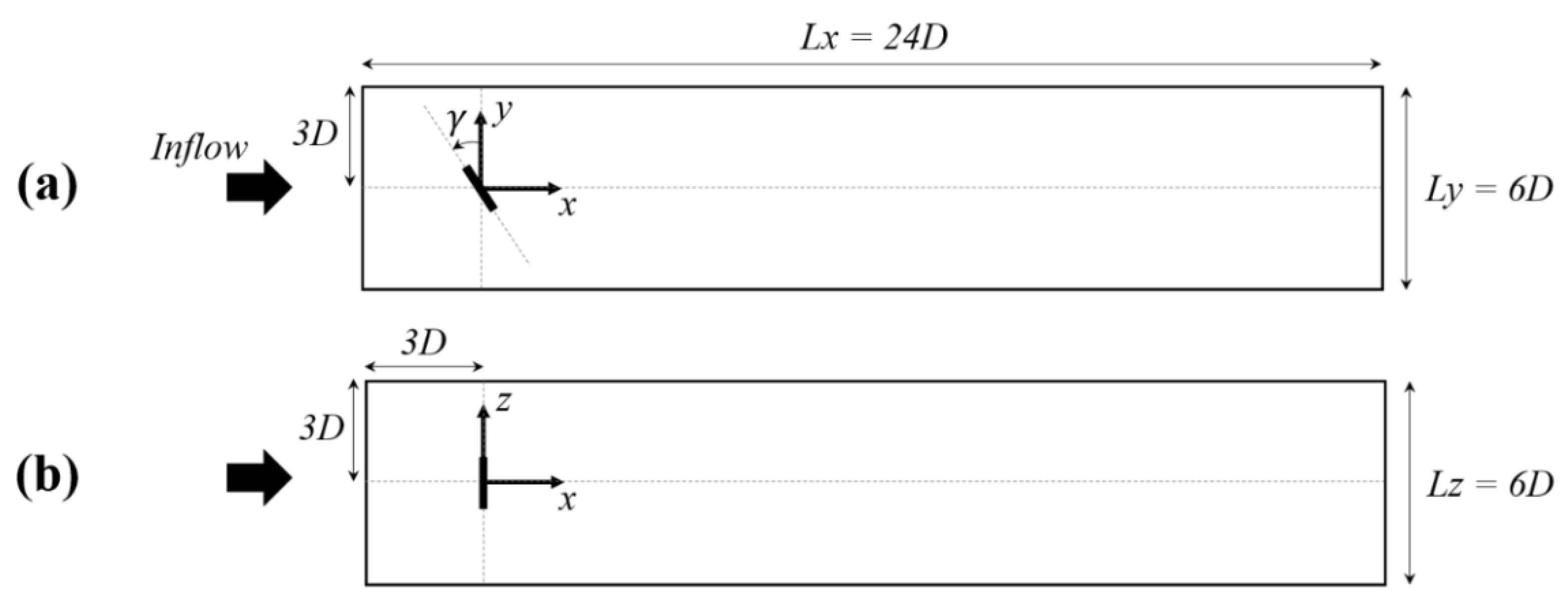
2.3. Simulation Set-Up

The domain used in the LES study is shown in Figure 1. $D$ denotes the diameter of the rotor, equal to 126 m. The size of the domain is $\left(L_x, L_y, L_z\right)=\left(24D, 6D, 6D\right)$, where x is the streamwise direction, y is the spanwise direction, and z is the vertical direction. The grid cell sizes were uniform and equal in all directions ($∆x=∆y=∆z=∆$, $∆/D=0.03125$). The numbers of the grid points were $\left(n_x, n_y, n_z\right)=\left(768, 192, 192\right)$, and the number of the total grid points was 28,311,552. The grid resolution used in the present study was sufficient to capture the curled wake structure, and the result mentioned in Section 3 was in close agreement with the previous studies in terms of the wake deformation, trajectories, and skewed angles [7,14].

The origin was located at a position $3D$ away from the boundaries where the actuator disk (AD) is positioned. The yaw angle ($\mathsf{\gamma }$) was defined as positive in the counterclockwise direction, as shown in Figure 1a. In the downstream view, the direction of the rotor rotation is clockwise. In order to focus on the wake generated by yawed rotor blades, the presence of the hub was neglected, allowing the flow to freely pass through the center of the AD. Likewise, the nacelle and tower were also excluded from the simulations. In a previous study, improved results were obtained when the nacelle and tower were included in the simulations [26]. However, the improvements, such as the wake profiles, were marginal and delivered no significant difference compared to simulations without the nacelle and the tower. In addition, these hardware components were noncritical in the formation of the curled wake structure. As such, the turbine model excluded the nacelle and tower in order to focus on the curled wake structure formed by the yawed rotor.

In the streamwise direction, the Dirichlet condition and the outflow condition were imposed on the inlet and outlet, respectively. In the spanwise and vertical directions, the cyclic condition was used. In this study, simulations were performed with various yaw angles with a uniform inflow condition. Numerous studies have included the ground with a targeted surface roughness to generate the sheared wind profile, which yielded visible differences in the wake field compared with a uniform inflow [15,16]. However, the wind shear was not a critical factor that contributes to the formation of the curled wake. Therefore, the wind shear was excluded in the present study to better understand the curled wake formation induced by the yaw angle in an isolated environment. The simulation cases are summarized in

Table 2. The cases of the simulation.

Inflow Wind Speed, ${\mathit{U}}_{\infty }$ [$\mathbf{m}{\mathbf{s}}^{-1}$]	Yaw Angle, $\mathsf{\gamma }$ [$°$]
9	−30, −20, −10, 0, 10, 20, 30

. The inflow wind speed, $U_{\infty }$, was set at 9 m/s. The yaw angles ranged from −30° to 30° with 10° increments.

3. Results and Discussion

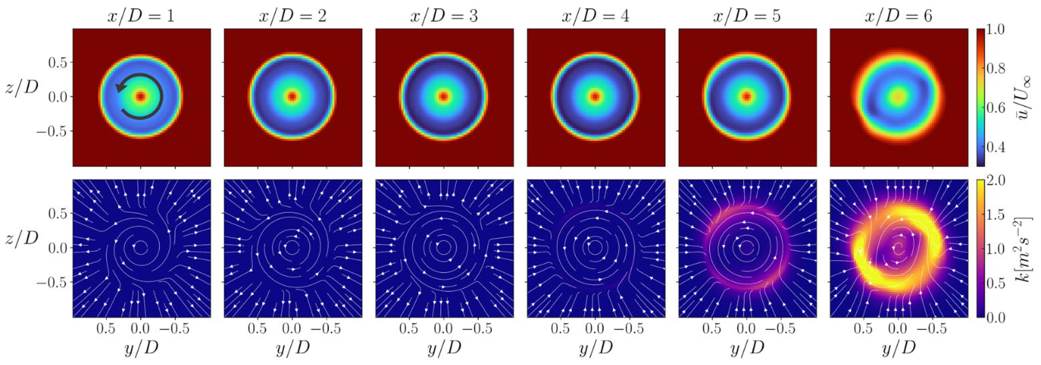
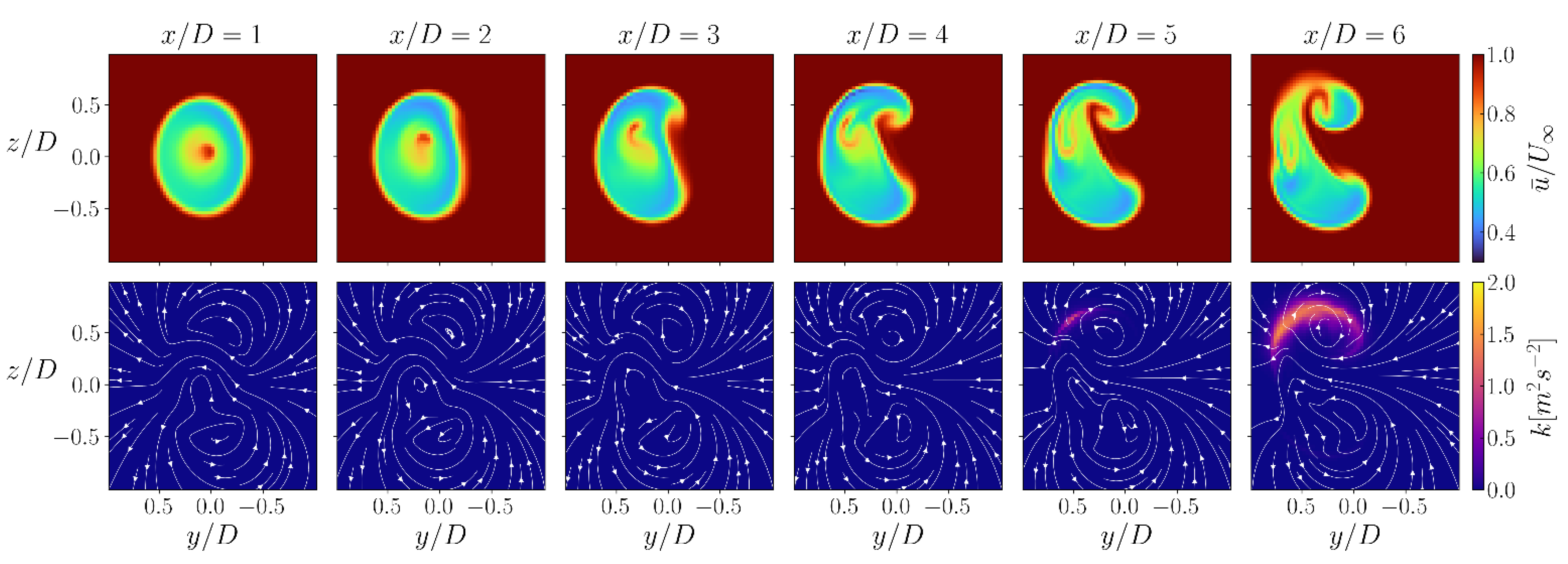
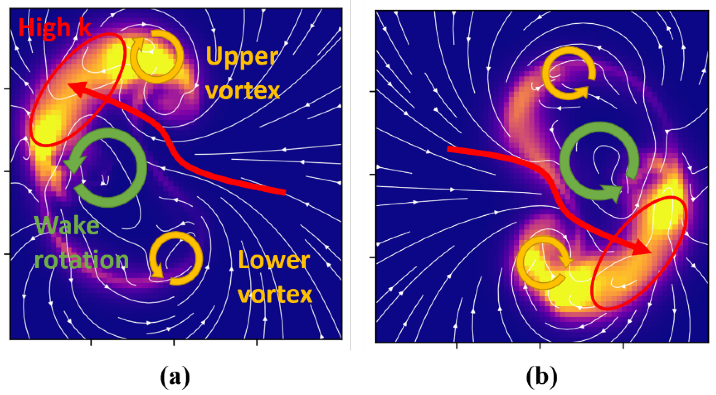
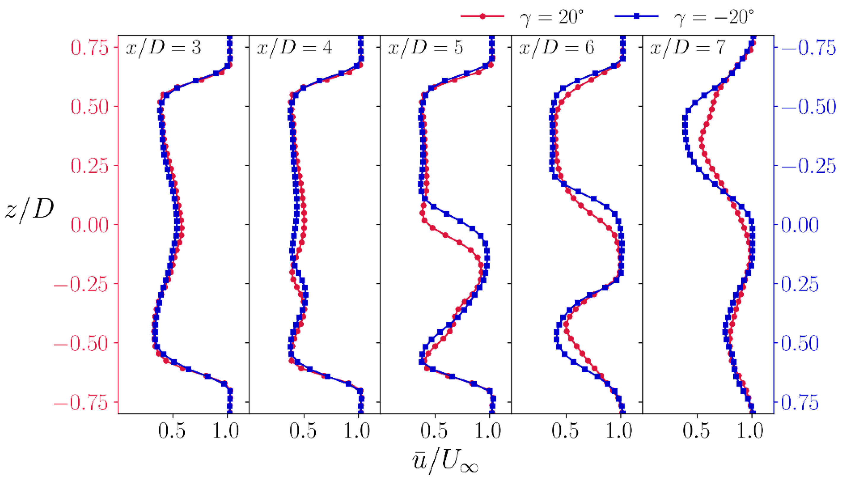
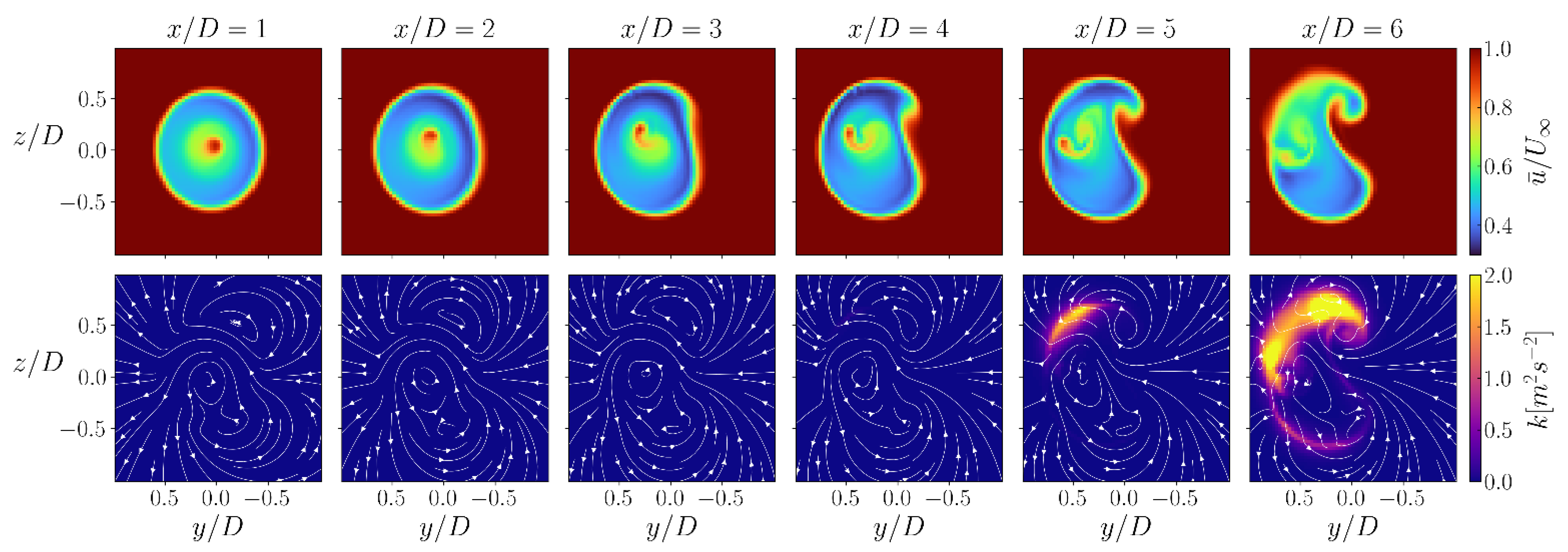
3.1. Streamwise Velocity Fields and Turbulent Kinetic Energy

In this section, the results for the streamwise velocity, the streamlines based on the time-averaged spanwise and vertical velocities, and the turbulent kinetic energy with various yaw angles are discussed. The turbulent kinetic energy, $k,$ is calculated according to Equation (5):

$$k=\frac{1}{2}\overline{\left(u^{\prime }{}^2+v^{\prime }{}^2+w^{\prime }{}^2\right)}$$

(5)

Figure 2 shows the cross-section contours of the flow fields looking in the downstream direction at the various locations $\left(x/D=1,2,3,4,5,\mathrm{and}6\right)$ without yaw ($\mathsf{\gamma }=0°$). For the mean streamwise velocity, $\overline{u}$, the velocity deficit occurred except for the rotor center region as the hub model was not included. Up to $x/D=5$, the turbine wake maintained a circular shape. The rotating flow in the counterclockwise direction can be seen in the streamlines, which is consistent with the turbine wake rotating in the opposite direction of the rotor. In addition, the high values of the turbulent kinetic energy were concentrated at the edge of the wake, which was attributed to the mixing layer between the wake and the free stream.

When the yaw angle was $\mathsf{\gamma }=-20°$, the initiation of the breakdown of the circular wake can be seen in Figure 3. Up to $x/D=2$, the wake shape retained a stable elliptical structure as shown in the time-averaged streamwise velocity contour, although the counter-rotating vortex pair (CVP) had already emerged even at $x/D=1$. Further downstream, the wake gradually transformed into a kidney-shaped structure consistent with previous experimental studies [6,7]. As shown in Figure 3, the upper region of the wake experienced severe distortion in comparison to that of the lower region, which is similar to the previous ALM study [6]. The asymmetric deformation of the wake can be attributed to the interaction of the global wake rotation and the CVP. The lateral flow entered approximately at the midpoint between the CVP and curved upwards due to the global wake rotation, further mixing with the upper CVP, which intensified the turbulent kinetic energy in the upper wake region, as shown when $x/D=5$. In addition, turbulent mixing further intensified in the upper wake region as the lateral flow curving upward interacted with the free stream at the edge of the wake. At $x/D=6$, the concentrated turbulent mixing further intensified at the upper edge of the wake. When the yaw angle was set to $\mathsf{\gamma }=-30°$, the transition from the elliptical wake to the kidney shape accelerated, as shown in Figure 4, where the curled wake can be seen even when $x/D=3$. The concentrated turbulent kinetic energy also appeared on the upper wing of the wake structure, consistent with the previous study performed in the ABL condition [14].

Figure 5 shows the cross-section contours for the time-averaged streamwise velocity $\overline{u}$, the instantaneous streamwise velocity, $u,$ and the turbulent kinetic energy (TKE), $k,$ at the distance of $x/D=6$ with yaw angles of $\mathsf{\gamma }=0°,-10°,-20°,\mathrm{and}-30°$. The deformation speed of the initially elliptical wake can be clearly seen as the lateral flow entering the wake region (shown by the streamlines) from the right side became stronger. On the other hand, the reduction in the wake deficit can be observed with higher yaw angles. The increase in the misalignment with the wind direction reduced the rotor’s thrust force, which weakened the velocity deficit, and this may have contributed to the reduced mixing within the wake region, causing the TKE to decrease.

The conjugate pairs of wakes resulting from the opposite yaw angles ($\mathsf{\gamma }=-20°\mathrm{and}20°$) are shown in Figure 6. The shape of the turbine wake was symmetrical about the original wake center. The high TKE at the lower wake edge ($\mathsf{\gamma }=20°$) was symmetrically consistent with the result from the opposite yaw angle. As shown in Figure 7, the asymmetry in the upper and the lower wake structures seems to be enhanced by the lateral flow (see streamlines) being entrained by the CVP and the global rotation of the wake structure, which contributed to the TKE concentrations in the upper and the lower parts of the wake region for each respective yaw angle.

Figure 8 shows the vertical profiles of the mean streamwise velocity, $\overline{u,}$ at $y=0$ at the various downstream distances ($\frac{x}{D}=3, 4, 5, 6, \mathrm{and} 7$) for the two yaw angles: $\mathsf{\gamma }=20°\mathrm{and}-20°$. When the velocity profile from the negative yaw angle case was inverted along the z-axis (in the vertical direction) for comparison, good agreement in terms of the overall shape was observed, and the wake rotation (same rotational direction regardless of the signs of the yaw angle) had a small impact on altering the wake development which is consistent with the findings of Kleusberg et al. [12]. Similar results were observed for the yaw angle pairs of $\mathsf{\gamma }=30°\mathrm{and}-30°$, as shown in Figure 9.

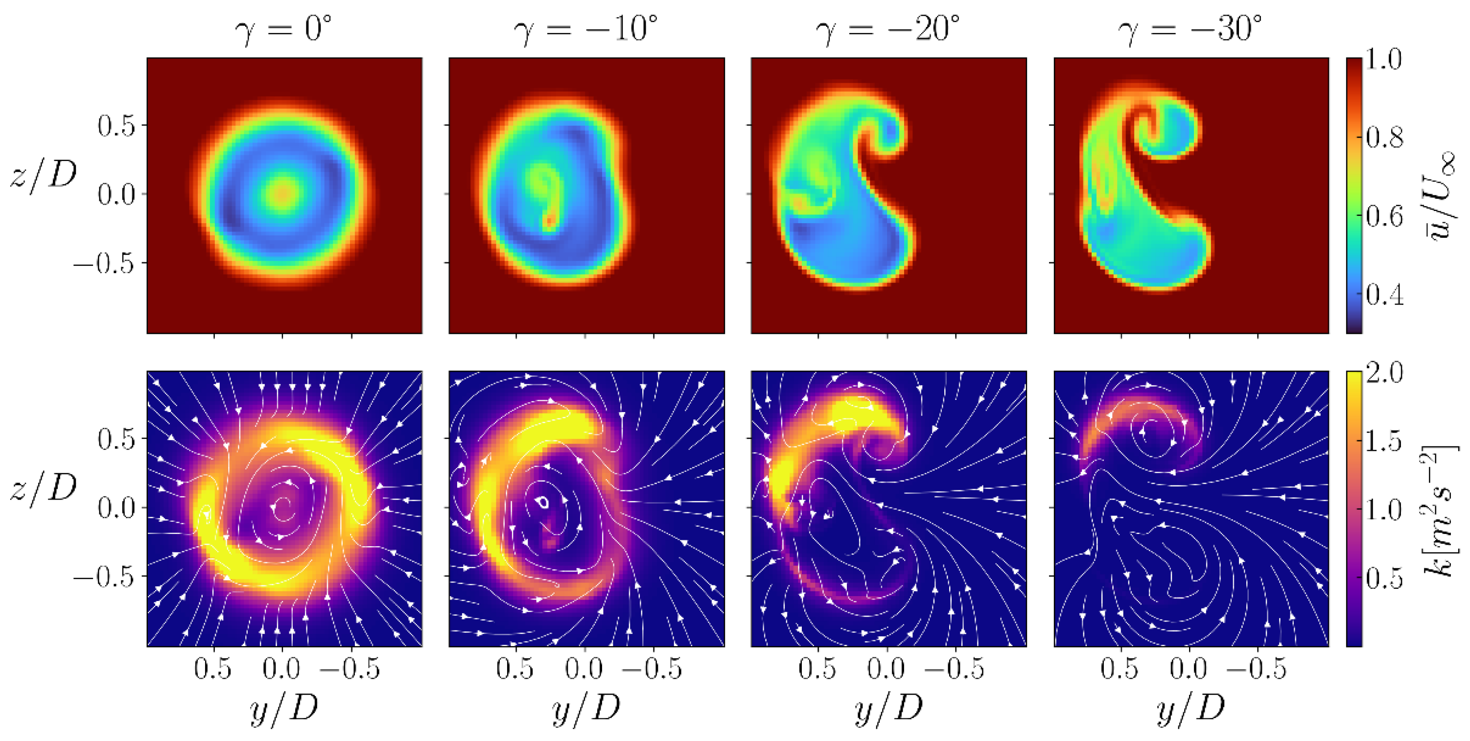
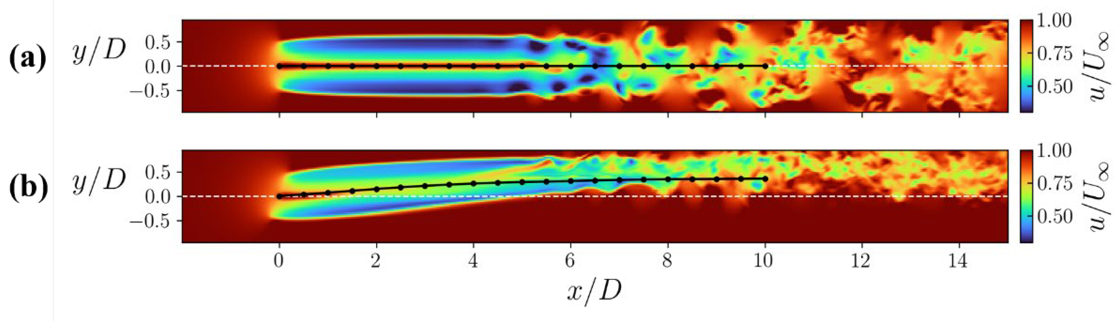
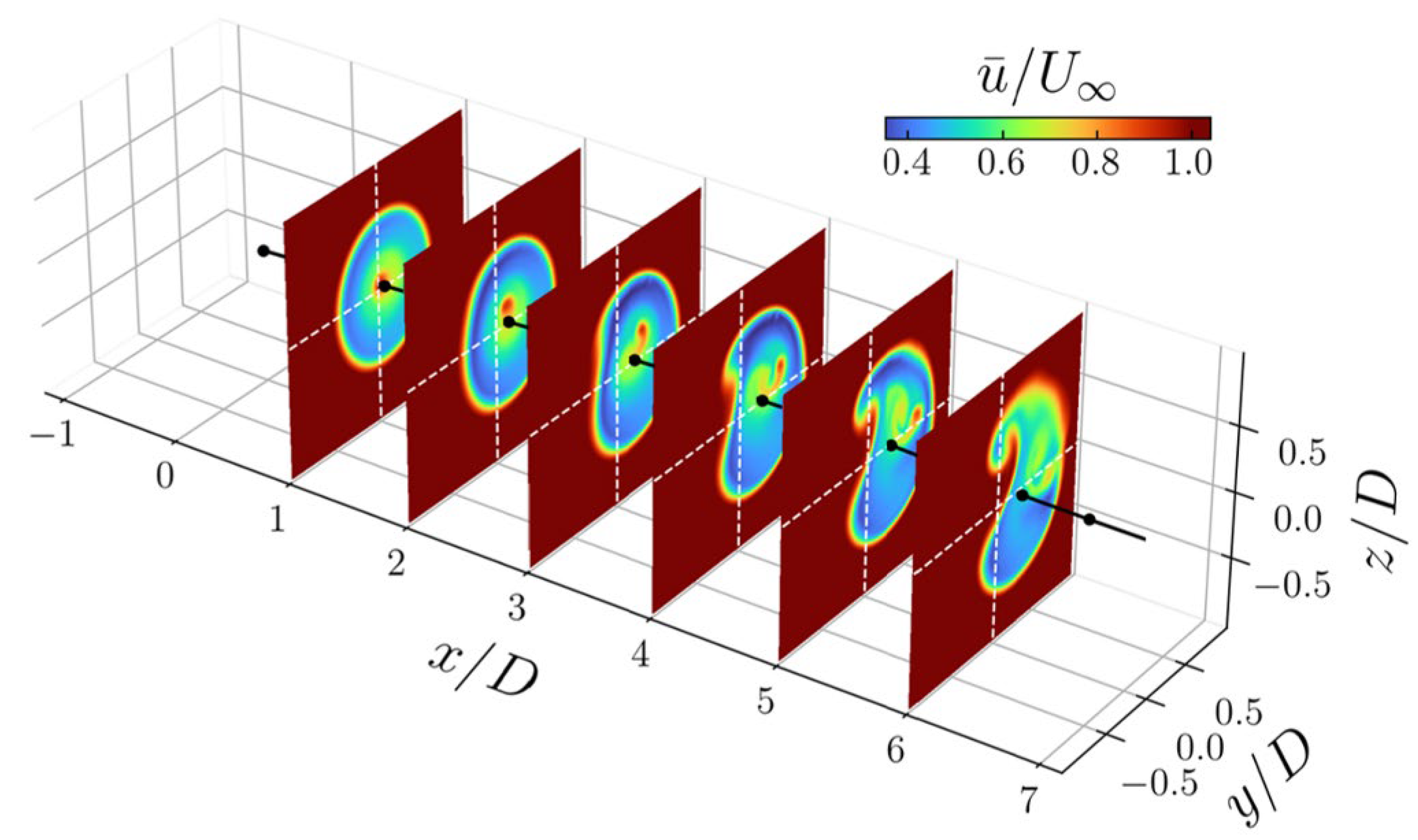
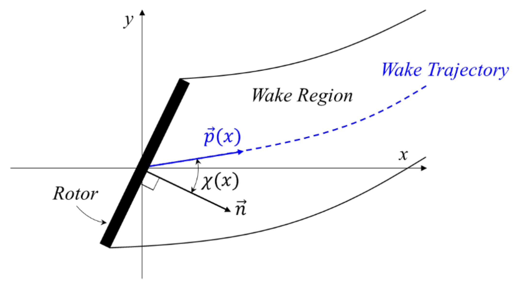
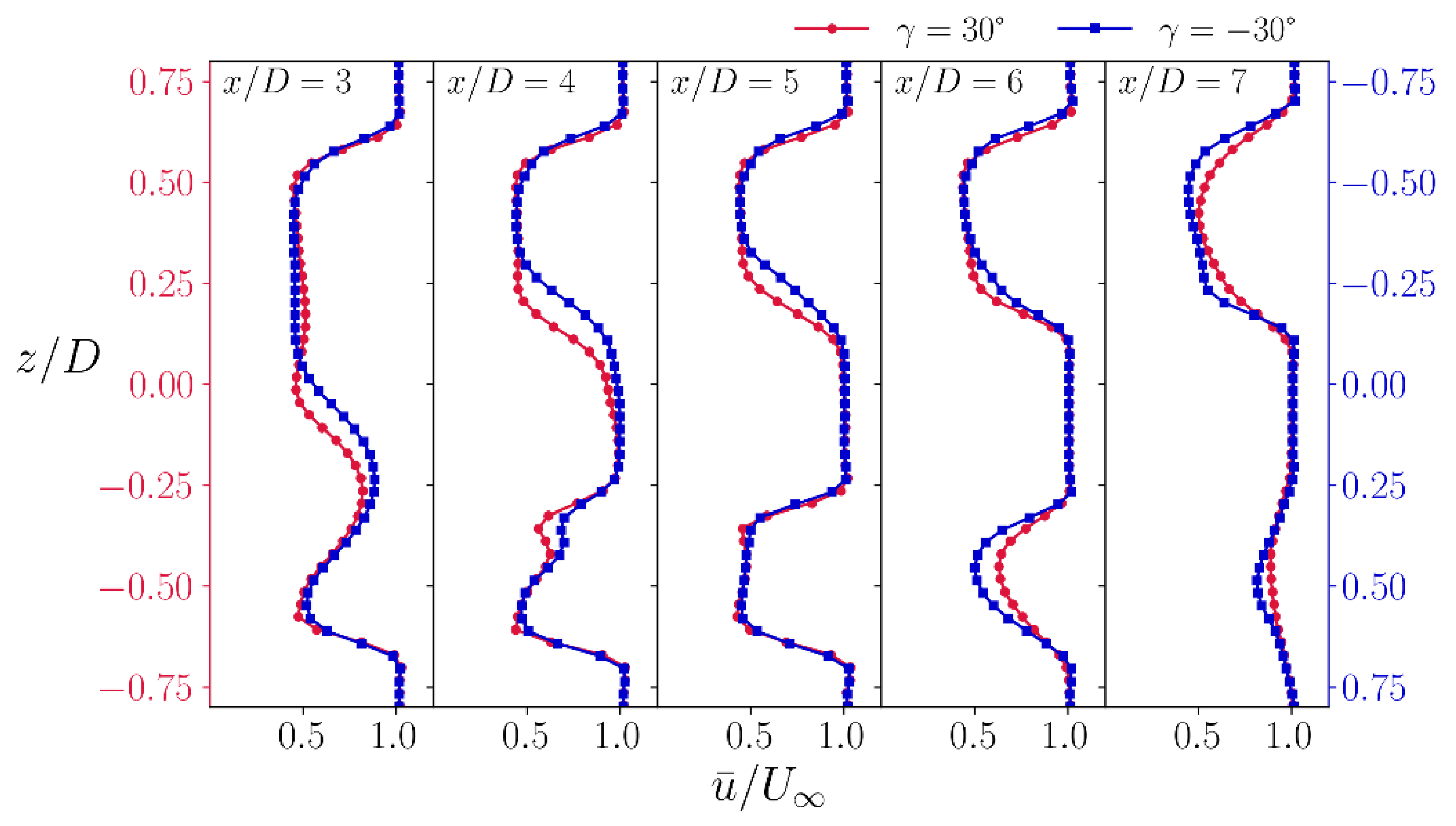
3.2. Wake Centerlines and Skew Angles According to Yaw Angles

To calculate the wake centerline, area-weighted average velocity deficit was used [6,27]. Figure 10 shows the top-view contours of the instantaneous streamwise velocity with two yaw angles $\mathsf{\gamma }=0°\mathrm{and}-20°$ taken at the center of the domain ($z=0$). With no yaw ($\mathsf{\gamma }=0°$), the wake centerline was maintained at the center position along the streamwise direction. On the other hand, the wake trajectory clearly deflected towards the spanwise direction with the yaw angle of $\mathsf{\gamma }=-20°$. As shown in Figure 11, it can also be seen that there was downward vertical movement. The size reduction of the wake was attributed to the interaction between the shear layer at the edge of the wake and the rotating actions of the CVP within the wake. In addition, the global rotation of the wake enhanced the upward entrainment of the lateral flow entering the cusp between CVP, which attributed to stronger mixing at the top CVP, as was seen in Figure 7. This mixing further reduced the upper wake area, which consequently resulted in the computed wake center shifting below the vertical centerline.

For a more quantitative analysis, the skew angles were calculated using the wake center trajectories. The skew angle ($\chi$) was defined as the angle between the position vector ($\overrightarrow{p}$) and the normal vector ($\overrightarrow{n}$) in the $xy$-plane, as shown in Figure 12 and Equation (6) [28,29]:

$$\chi \left(x\right)=co{s}^{-1}\left(\frac{\overrightarrow{p}\left(x\right)·\overrightarrow{n}}{\Vert \overrightarrow{p}\left(x\right)\Vert \Vert \overrightarrow{n}\Vert }\right).$$

(6)

where $\overrightarrow{p}$ is the vector from the center of the rotor to the wake trajectory line, and $\overrightarrow{n}$ is the normal vector of the rotor disk rooted at the rear face of the disk. Figure 13 shows the skew angles calculated with the various yaw angles ($\mathsf{\gamma }=-30°–30°$). In general, the skew angles obviously increased with the yaw angle input. The maximum skew angle appeared approximately at $x/D=2$, after which point the skew angles slowly decreased downstream, which shows that the efficacy of the wake redirection is most pronounced in the near wake region. The benefits of the wake redirection were clearly seen with the high yaw angle cases. However, these benefits were constrained within the near wake region, and the skew angle diminished after $x/D=3~4$ due to the wake recovery action. The discrepancies between the results from the opposite yaw angle pairs are presumed to be caused by the global wake rotation as the direction of the wake rotation was not mirrored. Larger yaw angle input increased this discrepancy, which slowly increased along the downstream positions.

4. Conclusions

In the present study, the curled wake structure behind a yawed wind turbine subjected to uniform inflow conditions ($U_{\infty }=9\mathrm{m}{\mathrm{s}}^{-1}$) was investigated using LES. The wake of the NREL 5 MW reference turbine model fixed with various yaw angles ($\mathsf{\gamma }=-30°~30°$) was numerically studied in which the presence of the turbine was implemented in the form of a rotating actuator disk. With the imposed yaw angle at the rotor, the circular wake deformed into an elliptical shape in the near wake and transformed into a kidney-like structure further downstream before the turbulent mixing occurred. The shape transition to the curled wake structure was accelerated with increasing yaw magnitude, which typically occurred at $x/D=3~5$ in the cases studied. The level of turbulent kinetic energy rapidly increased in the subsequent space as the breakdown of the curled wake initiated. In particular, high levels of turbulence were produced near the upper wake boundary in the case of the negative yaw angles. As the yaw angle increased, the degree of deformation of the wake structure and the deflection path further diverged in the near wake region. On the other hand, reductions in the velocity deficit and the turbulent kinetic energy were seen due to the decrease in thrust at a high yaw angle. The shape of the wake largely evolved in point symmetry about the center of the rotor for yaw angles of opposite signs despite the same rotational direction of the rotor, which indicated that the impact of rotation was minute in the wake distortion. However, the wake rotation resulted in a visible difference in the skew angle of the wake trajectory at high yaw angles.

References

1. Mechali, M.; Barthelmie, R.; Frandsen, S.; Jensen, L.; Rethore, P.E. Wake effects at Horns Rev and their influence on energy production. EWEC 2006, 1, 10–20. [Google Scholar]
2. Jiménez, Á.; Crespo, A.; Migoya, E. Application of a LES technique to characterize the wake deflection of a wind turbine in yaw. Wind Energy 2010, 13, 559–572. [Google Scholar] [CrossRef]
3. Fleming, P.; Churchfield, M.; Scholbrock, A.; Clifton, A.; Schreck, S.; Johnson, K.; Wright, A.; Gebraad, P.; Annoni, J.; Naughton, B.; et al. Detailed field test of yaw-based wake steering. J. Phys. Conf. Ser. 2016, 753, 052003. [Google Scholar] [CrossRef]
4. Fleming, P.; Annoni, J.; Scholbrock, A.; Quon, E.; Dana, S.; Schreck, S.; Raach, S.; Haizmann, F.; Schlipf, D. Full-scale field test of wake steering. J. Phys. Conf. Ser. 2017, 854, 012013. [Google Scholar] [CrossRef]
5. Doekemeijer, B.M.; Kern, S.; Maturu, S.; Kanev, S.; Salbert, B.; Schreiber, J.; Campagnolo, F.; Bottasso, C.L.; Schuler, S.; Wilts, F.; et al. Field experiment for open-loop yaw-based wake steering at a commercial onshore wind farm in Italy. Wind Energy Sci. 2021, 6, 159–176. [Google Scholar] [CrossRef]
6. Howland, M.F.; Bossuyt, J.; Martínez-Tossas, L.A.; Meyers, J.; Meneveau, C. Wake structure in actuator disk models of wind turbines in yaw under uniform inflow conditions. J. Renew. Sustain. Energy 2016, 8, 043301. [Google Scholar] [CrossRef]
7. Bastankhah, M.; Porté-Agel, F. Experimental and theoretical study of wind turbine wakes in yawed conditions. J. Fluid Mech. 2016, 806, 506–541. [Google Scholar] [CrossRef]
8. Shapiro, C.R.; Gayme, D.F.; Meneveau, C. Modelling yawed wind turbine wakes: A lifting line approach. J. Fluid Mech. 2018, 841, R1. [Google Scholar] [CrossRef]
9. Shapiro, C.R.; Gayme, D.F.; Meneveau, C. Generation and decay of counter-rotating vortices downstream of yawed wind turbines in the atmospheric boundary layer. J. Fluid Mech. 2020, 903, R2. [Google Scholar] [CrossRef]
10. Zong, H.; Porté-Agel, F. A point vortex transportation model for yawed wind turbine wakes. J. Fluid Mech. 2020, 890, A8. [Google Scholar] [CrossRef]
11. Schottler, J.; Bartl, J.; Mühle, F.; Sætran, L.; Peinke, J.; Hölling, M. Wind tunnel experiments on wind turbine wakes in yaw: Redefining the wake width. Wind Energy Sci. 2018, 3, 257–273. [Google Scholar] [CrossRef]
12. Kleusberg, E.; Schlatter, P.; Henningson, D.S. Parametric dependencies of the yawed wind-turbine wake development. Wind Energy 2020, 23, 1367–1380. [Google Scholar] [CrossRef]
13. Hamilton, N.; Suk Kang, H.; Meneveau, C.; Bayoán Cal, R. Statistical analysis of kinetic energy entrainment in a model wind turbine array boundary layer. J. Renew. Sustain. Energy 2012, 4, 063105. [Google Scholar] [CrossRef]
14. Lin, M.; Porté-Agel, F. Large-eddy simulation of yawed wind-turbine wakes: Comparisons with wind tunnel measurements and analytical wake models. Energies 2019, 12, 4574. [Google Scholar] [CrossRef]
15. Bartl, J.; Mühle, F.; Schottler, J.; Sætran, L.; Peinke, J.; Adaramola, M.; Hölling, M. Wind tunnel experiments on wind turbine wakes in yaw: Effects of inflow turbulence and shear. Wind Energy Sci. 2018, 3, 329–343. [Google Scholar] [CrossRef]
16. Hulsman, P.; Wosnik, M.; Petrović, V.; Hölling, M.; Kühn, M. Development of a curled wake of a yawed wind turbine under turbulent and sheared inflow. Wind Energy Sci. 2022, 7, 237–257. [Google Scholar] [CrossRef]
17. Maronga, B.; Banzhaf, S.; Burmeister, C.; Esch, T.; Forkel, R.; Frohlich, D.; Fuka, V.; Gehrke, K.F.; Geletič, J.; Giersch, S.; et al. Overview of the PALM model system 6.0. Geosci. Model Dev. 2020, 13, 1335–1372. [Google Scholar] [CrossRef]
18. Patrinos, A.N.A.; Kistler, A.L. A numerical study of the Chicago lake breeze. Bound.-Lay. Meteorol. 1977, 12, 93–123. [Google Scholar] [CrossRef]
19. Deardorff, J.W. Stratocumulus-capped mixed layers derived from a three-dimensional model. Bound.-Lay. Meteorol. 1980, 18, 495–527. [Google Scholar] [CrossRef]
20. Heinz, S. Realizability of dynamic subgrid-scale stress models via stochastic analysis. Monte Carlo Meth. Appl. 2008, 14, 311–329. [Google Scholar] [CrossRef]
21. Mokhtarpoor, R.; Heinz, S. Dynamic large eddy simulation: Stability via realizability. Phys. Fluids 2017, 29, 105104. [Google Scholar] [CrossRef]
22. Germano, M.; Piomelli, U.; Moin, P.; Cabot, W.H. A dynamic subgrid-scale eddy viscosity model. Phys. Fluids 1991, 3, 1760–1765. [Google Scholar] [CrossRef]
23. Wicker, L.J.; Skamarock, W.C. Time-splitting methods for elastic models using forward time schemes. Mon. Weather Rev. 2002, 130, 2088–2097. [Google Scholar] [CrossRef]
24. Wu, Y.T.; Porté-Agel, F. Large-eddy simulation of wind-turbine wakes: Evaluation of turbine parametrisations. Bound.-Layer Meteorol. 2011, 138, 345–366. [Google Scholar] [CrossRef]
25. Jonkman, J.; Butterfield, S.; Musial, W.; Scott, G. Definition of a 5-MW Reference Wind Turbine for Offshore System Development; Technical Report NREL/TP-500-38060; National Renewable Energy Laboratory: Golden, CO, USA, 2009. [Google Scholar]
26. Stevens, R.J.; Martínez-Tossas, L.A.; Meneveau, C. Comparison of wind farm large eddy simulations using actuator disk and actuator line models with wind tunnel experiments. Renew. Energy 2018, 116, 470–478. [Google Scholar] [CrossRef]
27. Bastankhah, M.; Porté-Agel, F. Wind tunnel study of the wind turbine interaction with a boundary-layer flow: Upwind region, turbine performance, and wake region. Phys. Fluids 2017, 29, 065105. [Google Scholar] [CrossRef]
28. Macrì, S.; Coupiac, O.; Girard, N.; Leroy, A.; Aubrun, S. Experimental analysis of the wake dynamics of a modelled wind turbine during yaw manoeuvres. J. Phys. Conf. Ser. 2018, 1037, 072035. [Google Scholar] [CrossRef]
29. Wagenaar, J.W.; Machielse, L.; Schepers, J. Controlling wind in ECN’s scaled wind farm. In Proceedings of the EWEA 2012, Copenhagen, Denmark, 16–19 April 2012. [Google Scholar]
Figure 1. The domain configuration for simulations: (a) top view, (b) side view.
Energies 15 06125 g001
Figure 2. The contours of the mean streamwise velocity fields, u , ¯ and the turbulent kinetic energy, k , with a yaw angle γ = 0 ° . The time-averaged streamlines are represented by white vector lines. The black arrow indicates the direction of wake rotation.
Energies 15 06125 g002
Figure 3. The contours of the mean streamwise velocity fields u ¯ and the turbulent kinetic energy, k , with a yaw angle γ = 20 ° . The time-averaged streamlines are represented by white vector lines.
Energies 15 06125 g003
Figure 4. The contours of the mean streamwise velocity fields u ¯ and the turbulent kinetic energy, k , with a yaw angle γ = 30 ° . The time-averaged streamlines are represented by white vector lines.
Energies 15 06125 g004
Figure 5. The contours of the mean streamwise velocity fields, u ¯ , the instantaneous streamwise velocity fields, u , and the turbulent kinetic energy, k , at a distance x / D = 6 with different yaw angles: γ = 0 ° , 10 ° , 20 ° ,   and   30 ° . The time-averaged streamlines are represented by white vector lines.
Energies 15 06125 g005
Figure 6. The contours of the mean streamwise velocity fields u ¯ and the turbulent kinetic energy k at the distance x / D = 6 with different yaw angles:   γ = 0 ° , 20 ° , and   20 ° . The time-averaged streamlines are represented by white vector lines.
Energies 15 06125 g006
Figure 7. Interaction of wake rotation and CVP in the contour at x / D = 6 : (a) γ = 20 ° ,   ( b )   γ = 20 ° .
Energies 15 06125 g007
Figure 8. Comparisons of vertical profiles of the mean streamwise velocity, u , ¯ at y = 0   with yaw angles γ = 20 °   (red circle) and γ = 20 °   (blue square).
Energies 15 06125 g008
Figure 9. Comparisons of vertical profiles of the mean streamwise velocity, u , ¯ at y = 0 with yaw angles γ = 30 °   (red circle) and γ = 30 °   (blue square).
Energies 15 06125 g009
Figure 10. The contours of the instantaneous streamwise velocity, u , with different yaw angles: (a) γ = 0 ° , (b) γ = 20 ° . The wake centerlines are represented by black lines.
Energies 15 06125 g010
Figure 11. The contours of the time-average streamwise velocity, u , ¯ with a yaw angle γ = 20 ° . The wake centerline is represented by a black line. The white dotted lines represent the centerlines ( y = 0 and z = 0 ).
Energies 15 06125 g011
Figure 12. The configuration of skew angle ( χ ) on the x y -plane.
Energies 15 06125 g012
Figure 13. Skew angles with various yaw angles of γ = 30 ° ~ 30 ° .
Energies 15 06125 g013