1. Introduction
The sharp growth of the Chinese economy has resulted in a dramatic increase in carbon emissions and energy demand in the last decades [
1,
2]. As the largest carbon emitter in the world, China has generated carbon emissions of 11.9 Gt, accounting for about 30% of global emissions [
3]. As the only country quickly recovering from the COVID-19 pandemic, electricity demand in China increased by 10% in 2021. The 56% rise in electricity demand in China required coal consumption [
3,
4], which makes it difficult to promote the progress of United Nations’ Sustainable Development Goal (SDG) 7, i.e., affordable and clean energy. The greenhouse gas generated by the household sector related to electricity and heating energy accounts for more than 30% of that by all sectors [
5]. Carbon emissions related to the household sector in China reached about 443.1 Mt in 2017, ranking fifth out of the forty-six sectors as a major source of carbon emissions. Moreover, the share of direct carbon emissions generated by the household sector experienced a sharp increase of more than 50% from 2007 to 2017, showing the great potential of household carbon emission growth in the future [
6]. It indicates that China has a huge challenge to achieve SDG 13, i.e., climate action from the perspectives of industrial sectors and the household sector [
7]. Hence, the interest in carbon mitigation policies targets inter-sectoral activities and household consumption.
The input–output (IO) framework has been used to investigate a wide variety of environmental issues associated with inter-sectoral activities based on the methodological extension of Leontief [
8], such as water flows, energy consumption, and carbon emissions [
9,
10,
11]. Lenzen et al. (2013) adopted a multi-region input–output table to evaluate virtual water flows embodied in international trade [
9]. Voigt et al. (2014) analyzed the trends and drivers of energy intensities in 40 economies based on the IO model and the Logarithmic Mean Divisia Index Decomposition [
10]. Mi et al. (2016) employed the IO model to calculate the production-based and consumption-based carbon emissions for thirteen Chinese cities and explored the carbon emissions embodied in inter-regional trade [
11]. In the classic Leontief IO theory, the output is driven by the final demand (e.g., household consumption expenditure, government consumption expenditure, gross capital formation, and exports). Household consumption has a one-way effect on the intermediate transaction among the industries in the conventional open IO model [
12], which only affects environmental issues as an exogenous factor. In fact, there are the mutual effects, rather than a one-way effect, between the industrial sector and the household sector. The intermediate transactions associated with the higher economic output could stimulate household consumption via growth in household income. The household sector acts as the main actor of final energy consumption, and the rise in household consumption leads to a significant increase in energy consumption and carbon emissions [
13]. Carbon emissions directly generated by the household sector are from the direct combustion of fossil fuels for household activities (e.g., cooking, clothing, and housing) [
14], which could be influenced by household income [
15]. Growing household income resulted in the enormous increase in energy consumption of the household sector over the last two decades, directly leading to a huge rise in carbon emissions [
16]. In addition, indirect emissions of the household are embedded in intermediate transactions [
14], indicating that the production sectors generate carbon emissions driven by household consumption.
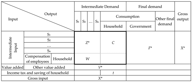
Based on the understanding of mutual effects, the semi-closed IO model can be constructed by moving household consumption and income into intermediate use, which treats the household as an endogenous factor. The semi-closed IO model with an endogenized household has been extended to investigate the environmental issues, such as seawater desalination, carbon emissions, and waste flows. Zou and Liu (2016) applied the semi-closed IO model to carry out an analysis of the economic effects of seawater desalination in China [
17]. Liao et al. (2017) integrated the semi-closed IO model with the modified hypothetical extraction method to quantify the net carbon linkages of sectors and households in Beijing [
18]. He et al. (2018) adopted the closed IO model to analyze the effect of the household sector on Australian waste flows [
19].
Most previous research on inter-industrial analysis is based on the Leontief demand-driven IO model, allocating the gross output to final demands. However, most policymakers focus on the economic structure or sectoral environmental performance from the perspective of value added rather than final demand [
20]. It is necessary to adopt the supply-side IO model to investigate the inter-industrial transaction enabled by various primary inputs, which is called the Ghosh IO model. The basic assumption of the supply-side IO model is that the output allocations in an economic system are stable [
21]. When there is an exogenous change in the value added, the allocation coefficients remain stable [
22]. In contrast to the Leontief inverse, the Ghosh inverse can be interpreted as the allocation structure, measuring the dependence of a particular sector on other sectors as a buyer of its output [
20,
23]. The Ghosh IO model has been applied to measure resource consumption and pollutant generation, including air pollutants, mercury emissions, and carbon emissions [
24,
25,
26]. Xie et al. (2018) adopted the Ghosh IO model to decompose the factors of air pollutants in China [
24]. Zhang et al. (2018) calculated the enabled and embodied mercury emissions in China, using income-based accounting and consumption-based accounting, respectively [
25]. Sajid et al. (2019) investigated the sectoral carbon linkages in Turkey from the demand and supply side [
26]. The semi-closed IO model tends to be applied to investigate demand-related carbon emissions, which reveals the inter-sectoral transaction of the sectors and the household driven by various final demands. Much less attention has been given to the supply-side carbon emissions with the household sector endogenized into the intermediate transaction.
Structural decomposition analysis (SDA) can investigate a wide range of technological effects and final demand effects in the IO model [
27]. As the SDA technique can identify the direct effect on carbon emissions as well as the indirect effect through the interactions among sectors, many scholars adopted SDA based on the IO model to quantify the contributions of several socioeconomic factors to changes in carbon emissions from the demand-driven perspective [
28,
29]. Su et al. (2017) carried out the first comprehensive analysis of Singapore’s carbon emissions by the IO model and the SDA technique and found that the emission growth was mainly driven by exports [
28]. Pu et al. (2020) decomposed China’s embodied carbon emissions based on SDA and found that the total trade volume was the primary driver of emission growth [
29]. On the other hand, the supply-side SDA of production-related carbon emissions have been conducted. Based on the Ghosh IO model, the supply-side SDA has been adopted to decompose several environmental indicators. Su and Ang (2015) used the multiplicative SDA to identify the supply-side driving effects of changes in the aggregate carbon intensity of China [
30]. Xie et al. (2018) adopted the additive SDA to decompose the changes in air pollutant emissions into the supply-side contributions of economic activities, economic structures, allocation structures, and emission intensity [
24]. Compared with the multiplicative decomposition form, the additive decomposition form is usually applied to decompose the change in the absolute indicator [
30]. Moreover, there are huge differences between the demand-side SDA results and the supply-side SDA results. Zhang (2010) found that the contribution of the supply-side economic structure to increases in carbon emissions was much larger than the contribution of the demand-side economic structure in 1992–2002 calculated by Peters et al. (2007) [
20,
31]. Zhang et al. (2018) discovered that the primary input structure in the supply-side SDA had greater effects on the mercury emission growth than the final demand structure in the demand-side SDA from 1997 to 2012 [
25].
There are two approaches to investigate the inter-sectoral linkages in the IO analysis, the conventional multiplier and the hypothetical extraction method (HEM). The backward linkage based on the Leontief IO model and the forward linkage based on the Ghosh model are the main multipliers to assess the significance of one particular sector to the whole economic system, which have been extended to the environmental issues. For example, He et al. (2019) identified the manufacturing sector with the largest energy consumption reduction potential based on the analysis of backward and forward linkage [
32]. However, the conventional multiplier, not weighed by production or demand, fails to reflect the production structure; it integrates the self-consumption into the backward and forward linkages [
33]. The modified HEM linkage analysis decomposes the total carbon emissions into four demand-side linkage effects, including internal effect (IE), mixed effect (ME), net backward linkage (NBL), and net forward linkage (FBL), which are helpful to describe the flows of carbon emissions in the economic system [
34]. Later on, Sajid and Gonzalez (2021) developed the theoretical basis and empirical evaluation method of linkage analysis purely based on the Ghosh IO model, which is named as the supply-side modified HEM (SMHEM); they applied SMHEM to investigate the carbon emission linkage in China, India, and the USA [
35].
To date, the effect of the household sector on carbon emissions has been given little attention due to limitations in the method and data, especially from the supply-side perspective. As the popular open IO model may underestimate the contribution of households’ carbon emissions by completely neglecting the mutual effect between the industrial sector and the household sector, it is meaningful to develop a supply-side framework to analyze the relationship between carbon emissions and the Chinese economy by combining the semi-closed IO model with the Ghosh IO model. It is conducive to systematically understand the drivers and linkages of the sectoral carbon emissions associated with the primary resource, which could intuitively shed light on the carbon emission abatement and the allocation structure shift.
In this paper, we analyze the drivers and linkages of carbon emissions of the industrial sectors and the household sector in the Chinese economy by firstly constructing an environmentally extended semi-closed Ghosh input–output model, which can reflect the mutual effects between the industrial sector and the household sector and the effect of primary inputs on carbon emissions. The key factors of changes in production-related carbon emissions are identified by adopting the remodified supply-side SDA. This paper also decomposes the production-related carbon emissions into several kinds of net carbon linkages induced by primary inputs, which could help to reduce carbon emissions by the adjustment and reconstruction of the allocation structure. The contributions of this paper include: (a) constructing a sufficiently innovative model, an environmentally extended semi-closed Ghosh input–output model, by integrating the semi-closed IO model with the Ghosh IO model; and (b) remodifying the existing supply-side SDA and the supply-side modified hypothetical extraction method (SMHEM) for investigating the driving force and net carbon linkage of sectors and the household.
The rest of the paper is structured as follows:
Section 2 explains the methodology used in this paper, as well as the data sources and processing;
Section 3 presents the accounting results, the contribution of driving forces, and net carbon linkages of the sectors and the household, as well as discusses the main findings; and
Section 4 lists the important conclusions and outlines the policy implications.
3. Results and Discussions
3.1. Direct and Indirect Effects of Enabled Carbon Emissions
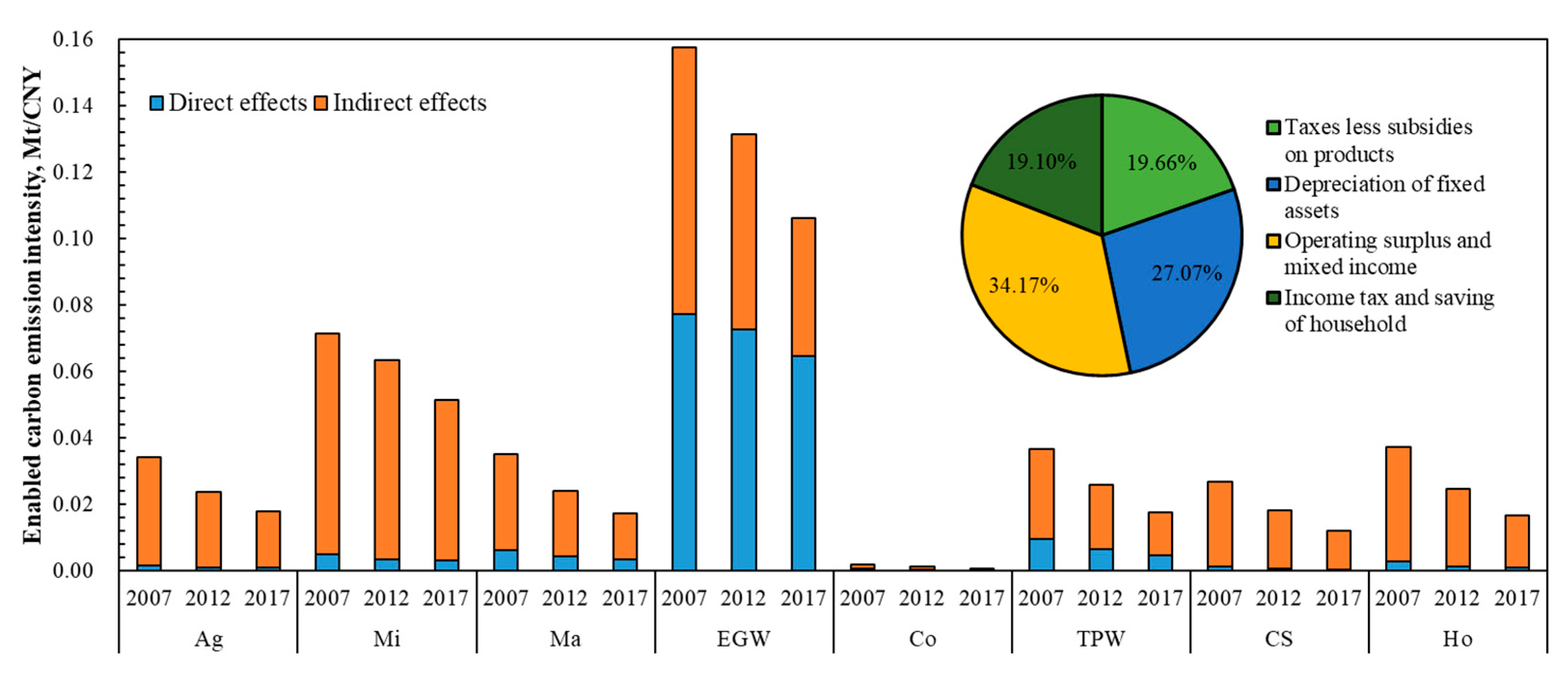
Figure 1 shows the sectoral carbon emission intensity and carbon emissions enabled by primary inputs in China. The bar chart shows the direct and indirect effects of the carbon emission intensity in eight sectors in 2007, 2012, and 2017. The pie chart illustrates the percentages of the carbon emissions enabled by four kinds of value added in 2017. The electricity, gas, and water supply sector had the largest enabled carbon emission intensity, at above 0.1 Mt/CNY. It indicates that the electricity, gas, and water supply sector generated more than 0.1 Mt carbon emissions with one CNY of primary inputs. This relatively high value of enabled carbon emission intensity was partly attributed to the largest direct emission intensity (direct effects) of more than 0.06 Mt/CNY. Coal-fired power is the major source of electricity and heating in China, which consumes coal to generate about two thirds of national electricity as of 2016 [
46,
47]. Therefore, the electricity, gas, and water supply sector became the major direct emission generator of the economic system. The emission intensity, as a ratio of direct emissions to the GDP, is an important indicator to reduce carbon emissions while preventing economic loss. Therefore, great importance should be attached to direct intensity reduction in the key industries, which is helpful to realize the decoupling of China’s economic growth from carbon emissions. Moreover, the high enabled intensity of the electricity, gas, and water supply sector is partly because most sectors are highly dependent on primary production, such as electricity, gas, and steam, which also had the greatest indirect effects of enabled carbon emissions. It indicates that the electricity, gas, and water supply sector generated huge carbon emissions enabled by its intermediate inputs from the downstream sectors.
After the electricity, gas, and water supply sector, the mining sector had comparatively high enabled intensity. As the mining sites are located in remote regions of China without the power grid, cleaner energy should be encouraged, including solar power, wind power, and biomass power. To manage the indirect carbon effects of the mining sector, the joint production of mining, refining, and metal production could improve efficiency of energy use and promote innovation of the technology and knowledge through the production chains. In addition, the household sector also had high enabled intensity, second only to the electricity, gas, and water supply sector and the mining sector.
Comparing direct and indirect effects of enabled carbon emission intensity, many sectors had more than 90% indirect effects out of the enabled carbon emission intensity, including the agriculture sector, the mining sector, the commercial and service sector, and the household sector. The mining sector had a comparatively high value of indirect effect, which was even larger than the indirect effect in the electricity, gas, and water supply sector in 2012 and 2017. The household sector had the third largest indirect effect of carbon emission intensity. Moreover, the household sector had more than 93% indirect effects out of its enabled intensities. It indicated that these sectors had huge demand for emission-intensive products as well as supplied their products as intermediate inputs to the other emission-intensive sectors downstream throughout the production chains. For the importance of indirect emission intensity enabled by primary inputs, the direct intensity of target sectors’ trading partners should be paid attention to. To be specific, carbon trading and taxation under the active government guidance may encourage the inter-sectoral cooperation of all the stakeholders and then reduce synergistic emissions.
Figure 1 also shows the trends in sectoral-enabled carbon emission intensity from 2007 to 2017. The enabled intensities of eight sectors all experienced a decrease. The household sector experienced a sharp decline in enabled intensity by more than 55% from 2007 to 2017. The carbon emission effects on the gross output via the supply chains with one CNY of primary inputs became weaker over the study period, indicating that the decoupling relationship between economic growth and carbon emissions has been developed.
The pie chart in
Figure 1 shows the shares of the carbon emissions enabled by four kinds of value added in 2017. Based on the semi-closed Ghosh IO model with an endogenized household sector, household income was treated as the intermediate input. Therefore, the primary inputs include taxes less subsides on products, depreciation of fixed assets, operating surplus and mixed income, and income tax and savings of households. The national enabled carbon emissions were mainly caused by the operating surplus and mixed income in 2017, resulting in 3214.67 Gt (34.17%) of enabled carbon emissions in China. As operating surplus and mixed income represents the capital income [
21], it indicated that capital had the most important role in carbon emissions in China from the value-added perspective.
3.2. Decomposition of Production-Related Carbon Emission Changes
Table 2 shows the driving effects of five socioeconomic factors on the changes in production-related carbon emissions in two periods of 2007–2012 and 2012–2017, including emission intensity (
), allocation structure (
), population size (
), economic activity (
), and economic structure (
).
Over the study period, emission intensity, allocation structure, and economic structure contributed to the reduction in production-related carbon emissions, while economic activity and population size resulted in carbon emission increase. In the first period from 2007 to 2012, economic activity (GDP per capita) caused the carbon emissions to increase by 84.10%, while population size had limited effects on carbon emission growth, at only 3.08%. Emission intensity had the largest contribution to production-related carbon emission reductions, resulting in a decrease of 33.60% in carbon emissions. By contrast, the driving effects of allocation structure and economic structure were much smaller, causing the carbon emissions to reduce by 7.36% and 7.51%, respectively. The combined contributions of economic activity and population size to carbon emissions were much higher than those of the remaining factors, increasing the carbon emissions by 38.71% in total. During the later period from 2012 to 2015, the impact of emission intensity became much weaker than that in the first period, reducing carbon emissions by 18.75%. Conversely, allocation structure offset more carbon emissions by about 16.49%. Moreover, economic activity, as the largest contributor to emission growth, brought only a 39.60% increase in carbon emissions. Therefore, production-related carbon emissions experienced a slight increase of 3.61% from 2012 to 2017. By contrast, the growth of production-related carbon emissions slowed down during the two stages.
The direct carbon emission intensity, as an important indicator of the cleaner production level, is always associated with the technological progress and specific sectoral technology characteristics [
48]. As is shown in
Figure 1, the direct emission intensity of all sectors experienced a decrease from 2007 to 2017, indicating a drop in carbon emissions per unit of the output. This is partly because advanced technology of energy saving and emission reduction has been promoted, and partly due to the elimination of backward capacity [
49]. Therefore, the improved energy consumption efficiency as well as capacity utilization rate brought the reduction in carbon emissions. Moreover, emission intensity showed a smaller contribution to offset carbon emissions, indicating that the efficiency advantage has been lost [
50]. This can be attributed to the slow-down trend of decline in sectoral emission intensity, especially the agriculture sector, the electricity, gas, and water supply sector, and the mining sector. The direct intensity of the agriculture sector even showed a slight increase from 2012 to 2017. The carbon emission abatement in the agriculture sector is not only a technical problem but also a socioeconomic issue [
51]. As the population size in China is stable, the gross output value in the agriculture sector experienced a slight increase of 26.63% from 2012 to 2017, much smaller than the growth rate of 77.47% from 2007 to 2012 [
45]. In the context of industrialization, the energy consumption increased with the wide use of the agricultural machinery [
52]. With active support and guidance from the government, farmers should also be encouraged to raise low-carbon awareness. On the other hand, the carbon sink function of crops is helpful to mitigate climate change [
53]. This result could shed light on carbon emission abatement throughout its life cycle, such as improving land-use efficiency, optimizing fertilization, and transforming straw into biomass energy.
As another component of the embodied intensity, allocation structure shows continuous improvement, with much stronger negative effects on carbon emissions during the later five-year period. Considering the communication of producers and markets, great attention should be given to allocation structure in macroeconomic control [
38]. Economic structure, representing the shares of sectoral primary input in the GDP, also brought emission reduction in the study, which was different from the economic structure effect based on the Leontief IO model [
20].
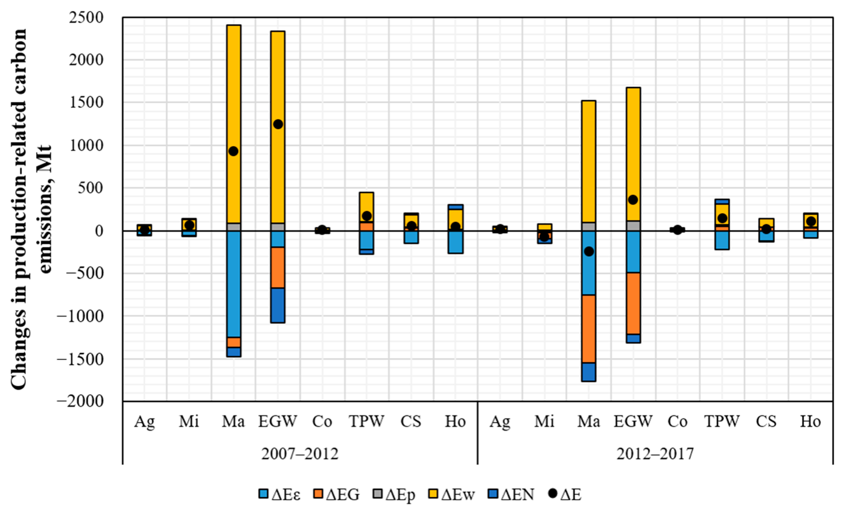
Figure 2 shows the contributions of five socioeconomic factors on the changes in production-related carbon emissions in eight sectors in two periods of 2007–2012 and 2012–2017.
Emission intensity brought the decrease in sectoral carbon emissions. It had the strongest driving effects in the manufacturing sector and the electricity, gas, and water supply sector, which both showed comparative strong direct effects of enabled carbon emission intensity. The reduction in carbon emissions associated with emission intensity in the manufacturing sector decreased, while that in the electricity, gas, and water supply sector increased. This could be explained by the decreased rates of emission intensity, as emission intensity of the electricity, gas, and water supply sector experienced a sharp decline from 2007 to 2017. Due to China’s efforts during the “12th Five-Year Plan” period (2011–2014), production capacity, including 1.55 million tons of steel, more than 600 million tons of cement, and 32.66 million tons of paper, has been eliminated, which brought the decline of direct carbon emissions in energy-intensive industries [
54].
Allocation structure was another factor with negative effects on carbon emissions in most sectors, and it had the largest contributions to reductions in carbon emissions in the manufacturing sector and the electricity, gas, and water supply sector from 2012 to 2017. It indicates that the value-added structure was beneficial for reductions in carbon emissions in emission-intensive sectors.
Population growth contributed to a slight increase in sectoral carbon emissions. There are two effects of population on carbon emissions. On the one hand, energy consumption may increase with population growth, thus generating more carbon emissions. On the other hand, technology development can be promoted, which can bring reduction in carbon emissions [
55].
Economic level was the greatest driving factor of increase in carbon emissions, and it had the most contributions in the manufacturing sector and the electricity, gas, and water supply sector.
The supply-side economic structure had unstable performance on changes in sectoral carbon emissions. Its contributions to generating carbon emissions declined, even shifting to reduce emissions in most sectors, except for the transport, postal, and warehousing sector. From 2007 to 2012, economic structure brought a reduction in carbon emissions in the transport, postal, and warehousing sector by 61.22 Mt. It had a positive effect on carbon emissions in the transport, postal, and warehousing sector, increasing emissions by 53.50 Mt. In this regard, economic structure from a value–added perspective should be further adjusted and optimized.
3.3. Supply-Induced Net Carbon Linkages
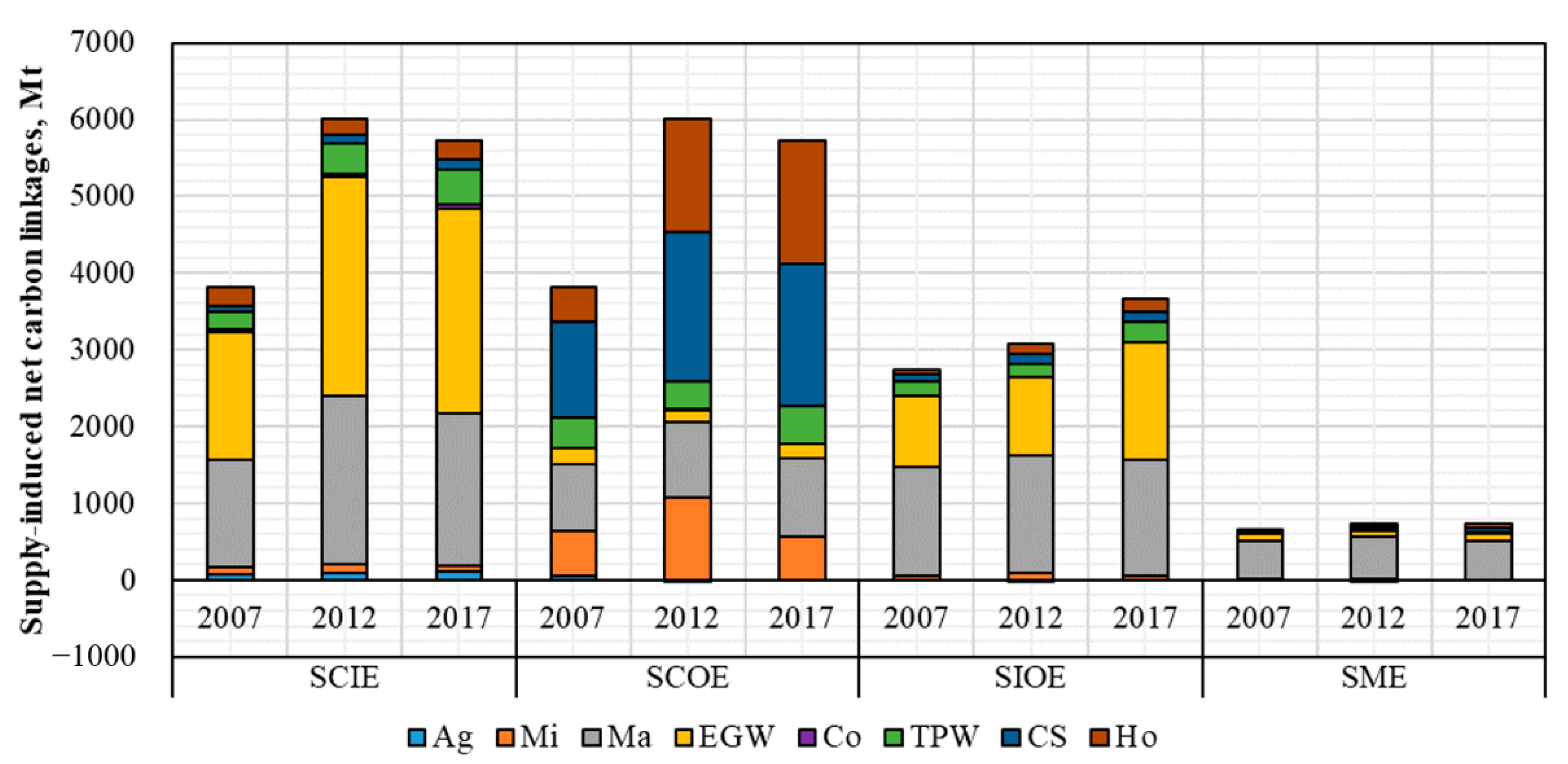
As the allocation structure in China has a strong driving effect on carbon emissions, the carbon emissions enabled by primary inputs were further decomposed into four kinds of supply-side net carbon linkages: supply-induced cross-sectoral input emissions (SCIE), supply-induced cross-sectoral output emissions (SCOE), supply-induced intra-sectoral output emissions (SIOE), and supply-induced mixed emissions (SME), as shown in
Figure 3. Cross-sectoral carbon emissions, including supply-induced cross-sectoral input emissions and supply-induced cross-sectoral output emissions, were the main components of net carbon linkages enabled by primary inputs, indicating that huge emissions were generated by inter-sectoral cooperation throughout the supply chains. Moreover, supply-induced intra-sectoral output emissions were also responsible for high enabled emissions, and their contribution to the total enabled emissions experienced an increase from 2007 to 2017 of 34.14%. This indicates that carbon emissions were generated in the closed circuits of one particular sector block, a result of the low degree of industry convergence. This result is also reported in studies focusing on the demand-side net carbon linkages, such as Liao et al. (2017) for Beijing [
18]. The supply-induced mixed emissions were comparatively lower, indicating that they have less importance in carbon emission abatement.
The top source of the supply-induced cross-sectoral input emissions in China was the electricity, gas, and water supply sector, accounting for more than 40% of the total supply-induced cross-sectoral input emissions. This is in line with the findings of the study for China, India, and the USA [
35]. It was mainly explained by the topmost direct emission intensity of the electricity, gas, and water supply sector. The manufacturing sector also generated huge supply-induced cross-sectoral input emissions, partly due to the great direct effects of enabled emissions. Another main factor of the supply-induced cross-sectoral input emissions was the primary inputs from other sectors, which enabled the manufacturing sector to generate the supply-induced cross-sectoral input emissions. Manufacturing industries are the core components of the economic activities in China [
56], which consume a large number of primary resources, such as electricity.
The commercial and service sector brought most of the supply-induced cross-sectoral output emissions, mainly due to its comparatively higher value added. Due to the assumption in the semi-closed IO model that the composition of employees has been moved into the intermediate sectors, the value added includes net taxes on production, depreciation of fixed assets, and operating surplus. In 2017, the value added of the commercial and service sector accounted for more than 32% of the total value added, while the percentage of its operating surplus to the total value was above 45%. As the economic development in China has entered into the “new normal” phase (roughly from 2014), the industry structure has oriented toward services and manufacturing with high value added. The tertiary industry may have huge potential to stimulate carbon emissions and resource consumption in energy-intensive sectors upstream throughout the supply chains. In addition, the household sector had high supply-induced cross-sectoral output emissions in 2012 and 2017 due to the increasing level of income tax and savings. It is evident that the household sector had small direct effects on enabled emissions, while its income tax and savings enabled other sectors to generate carbon emissions. Zhang and Wang (2017) reviewed the carbon abatement policies across the world and found that income level largely affects the choice of policy [
5]. Bai et al. (2021) attached importance to expanding consumption and increasing household income, which could lead to economic growth, job creation, and carbon abatement [
57]. Therefore, subsidies to households, and meanwhile levying a carbon tax, could stimulate household consumption as a significant component of the complementary measures of carbon tax.
The manufacturing sector was the top source of the supply-induced intra-sectoral output emissions, indicating that this sector generates high carbon emissions by using its own primary inputs. This was mainly due to that there are complex production–demand relationships among sub-sectors of the manufacturing sector. Most sectors consume the primary products after the elementary manufacture [
58]. While the allocation structure brought a decrease in carbon emissions in the manufacturing sector, a high degree of coordination among the sub-sectors should be advocated for.
4. Conclusions and Policy Implications
As production activities begin with primary resources, the reduction in carbon emissions of industrial sectors and the household sector enabled by the value added is practically meaningful to achieve China’s goals of carbon peak in 2030 and carbon neutrality in 2060. Considering the mutual effects between the industrial sector and the household sector, the semi-closed IO model was applied to investigate the carbon emissions, mainly based on the demand-driven Leontief IO model. For the production-related carbon emissions, this paper firstly integrated the semi-closed IO model with the Ghosh IO model to construct a new environmentally extended semi-closed Ghosh input–output model, which was applied to analyze the carbon emissions of the seven sectors and the household sector enabled by primary inputs in China. This paper remodified the supply-side SDA and SMHEM to quantitively analyze the driving force of the changes in the production-related carbon emissions as well as the four kinds of net carbon linkages. The conclusions in this paper are as follows.
First, the electricity, gas, and water supply sector was the key sector of the carbon emissions enabled by primary inputs. Most sectors generated huge indirect carbon emissions downstream throughout the production chains. In particular, the household sector had the great indirect effect, with its enabled intensity sharply decreasing. Among the four categories of the primary inputs, the operating surplus and mixed income representing the capital income made the largest contribution to the enabled emissions in 2017.
Second, the SDA results show that the emission intensity and allocation structure brought a dramatic decrease in carbon emissions, especially in the electricity, gas, and water supply sector. The population size and supply-side economic activity caused a rise in carbon emissions. Supply-side economic structure, calculated by the sectoral share of value added in GDP, contributed to the decrease in carbon emissions in most sectors, except for the transport, postal, and warehousing sector.
Third, the supply-induced cross-sectoral emissions were the major source of the production-related carbon emissions. At the sectoral level, the supply-induced cross-sectoral input emissions were the primary source in the electricity, gas, and water supply sector and the manufacturing sector, while the supply-induced cross-sectoral output emissions were the key linkage in the commercial and service sector and the household sector.
According to the main conclusions in this paper, the policy implications are as follows: (1) From the perspective of the whole production chain, when designing carbon trading and taxation, more attention should be paid to the responsibilities of the downstream and upstream sectors to improve the inter-sectoral cooperation and sharing of advanced technology and knowledge, such as the joint production of mining, refining, and metal. (2) As the emission intensity promoted the carbon emission abatement, the advanced technology and the elimination of backward capacity in the energy-intensive industries could have general value to realize the energy target in SDG 7 all over the world. For example, agricultural machinery should be guided while encouraging farmers to raise low-carbon awareness, which is significant in reconciling the food security related to SDG 2, i.e., zero hunger, with goals of carbon peak in 2030 and carbon neutrality in 2060. (3) As the economic structure in China has been oriented toward services and manufacturing with high value added during the “New Normal” phase, great importance should be attached to the commercial and service sector, due to its great potential to stimulate carbon emission generation in upstream sectors. According to the six climate-positive actions proposed by the UN Secretary-General [
59], the household sector, treated as an endogenous sector, should be complemented with subsidies when levying carbon taxes, which could help to realize economic growth, job creation, and carbon abatement at the same time.


