Article

Lead–Acid Battery SOC Prediction Using Improved AdaBoost Algorithm

1
Department of Power Manipulation, Navy Submarine Academy, Qingdao 266042, China
2
College of Engineering, Ocean University of China, Qingdao 266042, China
*
Author to whom correspondence should be addressed.
Energies 2022, 15(16), 5842; https://doi.org/10.3390/en15165842
Submission received: 16 July 2022 / Revised: 4 August 2022 / Accepted: 8 August 2022 / Published: 11 August 2022
(This article belongs to the Special Issue Modeling and Optimization Control of Power Battery)

Abstract

:
Research on the state of charge (SOC) prediction of lead–acid batteries is of great importance to the use and management of batteries. Due to this reason, this paper proposes a method for predicting the SOC of lead–acid batteries based on the improved AdaBoost model. By using the online sequence extreme learning machine (OSELM) as its weak learning machine, this model can achieve incremental learning of the model, which has a high computational efficiency, and does not require repeated training of old samples. Through improvement of the AdaBoost algorithm, the local prediction accuracy of the algorithm for the sample is enhanced, the scores of the proposed model in the maximum absolute error (AEmax) and maximum absolute percent error (APEmax) indicators are 6.8% and 8.8% lower, and the accuracy of the model is further improved. According to the verification with experimental data, when there are a large number of prediction samples, the improved AdaBoost model can reduce the prediction accuracy indicators of mean absolute percent error (MAPE), mean absolute error (MAE), and mean square error (MSE) to 75.4%, 58.3, and 84.2%, respectively. Compared with various other prediction methods in the prediction accuracy of battery SOC, the prediction accuracy indicators MAE, MSE, MAPE, AEmax, and APEmax of the model proposed in this paper are all optimal, which proves the validity and adaptive ability of the model.

1. Introduction

1.1. Background

Due to advantages in terms of mature production technology, high reliability, low production cost, and strong environmental applicability, lead–acid batteries have broad applications in various fields such as starters and portable power for vehicles, storage of excess energy from renewable sources, and backup or uninterrupted power supply systems [1]. Especially in terms of large-scale energy storage, lead–acid batteries remain to this day the most commonly found battery technology in operating microgrids [2]. The state of charge (SOC) of the battery refers to the ratio of the remaining capacity of the battery to the rated capacity, which not only reflects the remaining battery capacity, but also determines whether it can support the power use requirement of electrical equipment. Therefore, timely and accurate prediction of the SOC of lead–acid batteries is particularly important for the scientific use and health management of batteries [3].

1.2. Related Works

In both China and other countries, the battery SOC prediction models generally include the following four categories:
(1) The ampere-hour integration method [4,5,6]. According to the definition of battery SOC, this method obtains the SOC of the battery based on calculation of time integration after high-frequency sampling of battery power. This method has an open-loop mode. In [4], the current sensor is calibrated using the least square method, and the battery SOC is estimated using the ampere-hour integration method based on the estimation of available capacity and the power increment curve. In [6], to address the error caused by treating the battery capacity as a fixed value in the conventional ampere-hour analysis methods, a method is proposed to modify the capacity according to different discharge rate, coulombic efficiency, and temperature. The experimental results prove the effectiveness of this method. Although the ampere-hour integration method is simple and easy to calculate, this method has high requirements for the accuracy of the battery current measuring instrument, and the initial value of the battery SOC also needs to be accurate. This method can maintain high prediction accuracy within a short time, but with the increase in operating time, it is difficult to maintain high prediction accuracy for a long time due to the uncertainty of the coulombic efficiency and the error accumulation of the test current.
(2) The characteristic parameter method. This method predicts the SOC of the battery according to the mapping relationship between the open circuit voltage [7,8,9] or the internal resistance [10,11] of the battery and the remaining capacity of the battery. A non-steady-state open-circuit voltage method is proposed in [9], which can quickly estimate the battery SOC in real time. In [10], the internal resistance of a battery is calculated according to the law of energy conservation, and an improved SOC estimation method is proposed. In [11], state of charge (SOC) determination of a lead–acid battery cell by the electrochemical impedance spectroscopy (EIS) method is explored. In this type of methods, the measurement of the open-circuit voltage usually requires the battery to stand for a long time until it reaches a stable state. Moreover, the slope of the middle section of the mapping curve between the open-circuit voltage and the battery SOC is very small, and a small measurement error will lead to significant deviation in the SOC prediction. Therefore, this kind of method requires high prediction of the voltage sampling circuit, which is not suitable for real-time monitoring of the battery in practice. On the other hand, the measurement of battery internal resistance is affected by various factors, such as temperature, depth of discharge, and cycle times. It is difficult to achieve accurate and fast measurement of the battery internal resistance by using the general test equipment, which cannot meet the online prediction requirements of battery SOC.
(3) The mathematical model method. This method mainly predicts the SOC of the battery using two types of models based on the Kalman filter [12,13,14] and the particle filter [15,16,17] as well as their optimized and extended models. In [14], the state space equations are established and the extended Kalman filtering method is used for SOC estimation on the basis of the parameter identification results in the mathematical model. In [17], the particle filter algorithm is employed to predict the open-circuit voltage of the battery based on the first-order equivalent circuit model of the battery, and the mapping relationship between the open-circuit voltage and the SOC is established. Even though this kind of algorithm can provide accurate prediction of the battery SOC in some cases, because the performance of the algorithm heavily depends on the selection of the initial estimated value, if the initial estimated value involves significant deviation, the algorithm tends to converge slowly. Moreover, it also requires a large amount of sample data for support in order to achieve high accuracy of the algorithm.
(4) The data-driven method. This method predicts the battery SOC using a data-driven model. The data-driven methods mainly include: the artificial neural network [18,19,20], the extreme learning machine [21], and the support vector machine [22,23]. In [20], the battery SOC prediction model based on the back propagation (BP) neural network is trained by utilizing the relationships between the charge and discharge current and temperature of the battery and the SOC. In [23], a novel algorithm based on a robust extreme learning machine (RELM) optimized by the bird swarm algorithm is proposed to predict the SOC of a lead–acid battery, which overcomes the shortcoming that an extreme learning machine (ELM) cannot deal with outliers and improves the prediction accuracy of the ELM. The data-driven method does not require constructing a complex physical battery model, which has a strong non-linear fitting ability and strong robustness. This kind of method can provide excellent performances for various types of battery modeling, and is a popular method commonly used in recent studies on prediction of the battery SOC.

1.3. Limitations of Current Methods

This paper investigates the large-capacity flooded lead–acid battery, which is mainly used as a power source in large electrical equipment [24]. There are application schemes and environments of the battery in different equipment. During the use of the battery, parameters, such as current, voltage, charge and discharge time, electrolyte density, and electrolyte temperature, are sampled and recorded at fixed time intervals. The performance and health status of the battery will change continuously with its use, which will also affect the charge and discharge SOC of the battery. In prediction and research of the battery SOC, adaption to and tracking of the changes in the battery performance state are particularly important to the accurate prediction of the battery SOC.
Most current research methods for the battery SOC focus on the lithium batteries. Lead–acid batteries are significantly different from lithium batteries in terms of structural composition, working characteristics, application objects, and use processes [25,26]. Therefore, if the SOC prediction models for lithium batteries are directly used for prediction of large-capacity lead–acid batteries, it is difficult to provide accurate prediction, which is not applicable [27,28]. At the same time, the current prediction models for battery SOC are mostly static models constructed based on the previous state and usage data of the battery, which fail to consider the impact of battery performance changes on SOC during use, and such models generally lack the incremental learning ability for new battery samples. Therefore, it is necessary to optimize and improve the existing SOC prediction methods for lithium batteries or propose new data-driven methods, and equip these methods with the incremental learning ability and the ability to update adaptively and dynamically according to the changes in battery performance, so that such a method can be applied to the research object of this paper.

1.4. Research Method of This Paper

The AdaBoost algorithm is a representative ensemble learning algorithm of the data-driven methods, which has great advantages in non-linear system learning and prediction [29,30]. In this paper, improvement is made to the algorithm on the following aspects: study on the incremental learning ability of the weak learning machine and the optimization of the computation process of the AdaBoost algorithm. The improved AdaBoost algorithm uses the online sequence extreme learning machine (OSELM) as a weak learning machine. Through the incremental learning ability of the OSELM, the computational efficiency of the model in the incremental learning process is improved, and the tracking and learning and the performance change in the battery are realized, the update and modification of the model parameters are achieved, and the adaptive ability of the model is improved. By optimizing and improving the sampling and weight update processes in the original AdaBoost, the algorithm is more suitable for the data structure and distribution of our research object, and the prediction performance of the battery SOC is further improved. For the convenience of discussion, the proposed method is hereinafter abbreviated as the AdaBoost.I-OSELM method.

2. Related Deep Learning Theories

2.1. Extreme Learning Machine (ELM)

The extreme learning machine (ELM) is a feedforward neural network algorithm with single hidden layer, which randomly generates continuous weight between the input layer and the hidden layer and the threshold of neurons in the hidden layer. There is no need for adjustment during the training process, and a unique optimal solution can be obtained by setting the number of neurons in the hidden layer. Compared with conventional training methods, this method has the advantages of fast learning speed and good generalization performance [31].
A typical ELM neural network consists of the input layer, hidden layer, and output layer. The neurons between the input layer and the hidden layer, and between the hidden layer and the output layer, are fully connected. In this network, assume the input layer has n neurons, the hidden layer has l neurons, and the output layer has m neurons.
Assume a training set containing Q samples, the input matrix is X, and the corresponding output matrix is T, where:
X = [ x 11 x 12 x 1 Q x 21 x 22 x 2 Q x n 1 x n 2 x n Q ] n × Q ;   T = [ t 11 t 12 t 1 Q t 21 t 22 t 2 Q t m 1 t m 2 t m Q ] m × Q .
Let the activation function of neurons in the hidden layer be g(x), and the sigmoid, sin, or hardlim function is often chosen as the activation function. According to Figure 1, the output O of network is:
O = [ o 1 , o 2 , , o Q ] ,
o j = [ o 1 j o 2 j o m j ] m × 1 = [ i = 1 l β i 1 g ( w i x j + b i ) i = 1 l β i 2 g ( w i x j + b i ) i = 1 l β i m g ( w i x j + b i ) ] m × 1 ( j = 1 , 2 , , Q ) ,
where, ω is the connection weight matrix between the input layer and the hidden layer, and wji represents the connection weight between the i-th neuron in the input layer and the j-th neuron in the hidden layer. β is the connection weight matrix between the hidden layer and the output layer, and βjk represents the connection weight between the j-th neuron in the hidden layer and the k-th neuron in the output layer. b is the threshold of neurons in the hidden layer.
After transposing O, it can be represented as:
H β = O ,
where O is the transpose of matrix O , H is the output matrix of the hidden layer of the neural network, and its specific form is as follows:
H ( w 1 , w 2 , , w l , b 1 , b 2 , , b l , x 1 , x 2 , , x Q ) = [ g ( w 1 x 1 + b 1 ) g ( w 2 x 1 + b 2 ) g ( w l x 1 + b l ) g ( w 1 x 2 + b 1 ) g ( w 2 x 2 + b 2 ) g ( w l x 2 + b l ) g ( w 1 x Q + b 1 ) g ( w 2 x Q + b 2 ) g ( w l x Q + b l ) ] Q × l .
The ELM model training aims to minimize the prediction error of the model, so the loss function of training samples can be defined as:
f = O T = H β T ,
where T is the transpose of matrix T .
According to [23], the training error of the ELM algorithm can be approximated to an arbitrary ε > 0 , f = H β T < ε (only when the number of units in the hidden layer is equal to the number of training samples, f = H β T = 0 ). When the activation function g ( x ) is infinitely differentiable, w and b can be randomly selected before training and remain unchanged during training. The connection weight β between the hidden layer and the output layer can be obtained by solving the least squares of the following equations:
min H β T .
The solution is β = H + T . In it, H + is the Moore–Penrose generalized inverse of the output matrix of the hidden layer. In general, H T H is a non-singular matrix, so one can obtain:   H + = ( H T H ) 1 H T .

2.2. Online Sequence Extreme Learning Machine (OSELM)

The online sequence extreme learning machine (OSELM) algorithm is based on the neural network of the extreme learning machine (ELM). The model is trained offline using the existing training samples, and the output connection weights of the neural network are iterated and updated dynamically via incremental learning according to the newly acquired learning samples., which can minimize the computational burden, improve the update efficiency, and improve the prediction accuracy of the network. The update principle of this method is as follows [32].
Combining the ELM algorithm, when N1 new samples N 1 ^ = { ( x i , t i ) } i = N 0 + 1 N 1 are acquired for incremental learning, calculation of the new network output weight β 1  is equivalent to solving the minimum norm least squares of the new linear system, i.e.,
[ H 0 H 1 ] β ^ [ T 0 T 1 ] = min β [ H 0 H 1 ] β 1 [ T 0 T 1 ] ,
H 1 = [ g ( w 1 · x N 0 + 1 + b 1 ) g ( w 2 · x N 0 + 1 + b 2 ) g ( w l · x N 0 + 1 + b l ) g ( w 1 · x N 0 + 2 + b 1 ) g ( w 2 · x N 0 + 2 + b 2 ) g ( w l · x N 0 + 2 + b l ) g ( w 1 · x N 0 + N 1 + b 1 ) g ( w 2 · x N 0 + N 1 + b 2 ) g ( w l · x N 0 + N 1 + b l ) ] N 1 × N , T 1 = [ t N 0 + 1 T t N 0 + 2 T t N 0 + N 1 T ] T
where:
We can obtain β 1 = K 1 1 [ H 0 H 1 ] T [ T 0 T 1 ] , where:
K 1 = [ H 0 H 1 ] T [ H 0 H 1 ] = [ H 0 T H 1 T ] [ H 0 H 1 ] = K 0 + H 1 T H 1 ,
[ H 0 H 1 ] T [ T 0 T 1 ] = H 0 T T 0 + H 1 T T 1 = K 0 K 0 1 H 0 T T 0 + H 1 T T 1 = ( K 1 H 1 T H 1 ) β 0 + H 1 T T 1 = K 1 β 0 H 1 T
By using β 0 to represent β 1 , we can obtain:
β 1 = K 1 1 [ H 0 H 1 ] T [ T 0 T 1 ] = K 1 1 ( K 1 β 0 H 1 T H 1 β 0 + H 1 T T 1 ) = β 0 + K 1 1 H 1 T ( T 1 H 1 β 0 ) .
Similarly, when Nk+1 training samples N k + 1 ^ = { ( x j , t j ) } i = ( j = 0 k N j ) + 1 j = 0 k + 1 N j  are updated for the (k + 1)-th time, the network output weight can be iteratively calculated as:
K k + 1 = K k + H k + 1 T H k + 1 β k + 1 = β k + K k + 1 1 H k + 1 T ( T k + 1 H k + 1 β k ) .
According to the Woodbury principle [33], K k + 1 1 can be rewritten as:
K k + 1 1 = ( K k + H k + 1 T H k + 1 ) 1 = K k 1 K k 1 H k + 1 T ( I + H k + 1 K k 1 H k + 1 T ) 1 × H k + 1 K k 1 .
Let P k + 1 = K k + 1 1 , then the above equation can be rewritten as:
P k + 1 = P k + P k H k + 1 T ( I + H k + 1 P k H k + 1 T ) 1 × H k + 1 P k β k + 1 = β k + P k + 1 H k + 1 T ( T k + 1 H k + 1 β k ) .
Therefore, with the continuous increase in newly acquired samples, the online iterative update process of the connection weights of the OSELM neural network can be completed by the above equation, and the incremental learning ability of the model can be realized.
As a weak learning machine in the AdaBoost.I-OSELM method, the process to learn and predict the samples by using the OSELM is shown in Figure 1, which mainly includes the following steps:
(1) Initialize related parameters of the model, such as the number of nodes h at the hidden layer of the OSLEM, the number of new samples p corresponding to each update and the activation function f.
(2) Learn the OSELM model offline by training the samples.
(3) The model predicts the test samples according to the time sequence, and records the test samples as newly acquired learning samples during the prediction process.
(4) Calculate whether the number of newly acquired learning samples has reached the number of new samples required for one update of the model. If so, dynamically update the model parameters through the new samples, enter the online learning stage, and complete the incremental learning process of the model. If not, go to Step 3.
(5) Clear the number of newly acquired samples and go to Step 4, until the prediction and incremental learning of all test samples are completed.

2.3. AdaBoost Algorithm

The AdaBoost algorithm is a representative ensemble learning algorithm, which is an iterative boosting algorithm. In this algorithm, the predicted output of the weak learning machine generated by each iteration is compared with the actual output, and the weight of the current training sample and the weight of the current weak learning machine in the composite predictor are updated according to the difference between the predicted output and actual output. After iterating and updating the training samples for the next weak learning machine, the prediction analysis is performed again until the last weak learning machine stops. Therefore, the AdaBoost algorithm mainly combines the outputs of multiple “weak” learning machines to form the final “strong” prediction, that is, to generate accurate predictions [34,35].
The AdaBoost algorithm was originally a classification method. With the improvement of this method, it can also perform regression prediction now. At present, the classification algorithms developed based on AdaBoost mainly include the AdaBoost basic algorithm, AdaBoost.M1, and AdaBoost.M2, which are suitable to address discrete classifications that involve two or more classes. The algorithms that can perform regression prediction mainly include AdaBoost.R2 and AdaBoost.RT [36,37]. Taking the AdaBoost.R2 algorithm capable of regression prediction as an example, the main steps of its prediction process are as follows [30]:
(1) For the M groups of training samples { ( X i , Y i ) } i = 1 M in the sample training set, the initial distribution weight of the training data is assigned as D t = 1 ( i ) = 1 / M , assuming that T iterations are performed, and the number of initialization iterations is t = 1.
(2) Carry out cycle training of t = 1, 2, …., T.
① Train the sample, and obtain the weak learning machine f t ( x ) . Calculate the maximum error E t = m a x t | O t i Y t i | , ( i = 1 ,   2 M ) of the weak learning machine f t ( x ) on the sample data, where, O t i is the prediction result on training set Xi by the weak learning machine f t ( x ) .
② Calculate the relative error of the weak learning machine f t ( x ) on each sample, which can be the linear error, square error, or exponential error.
③ Calculate the error rate of the weak learning machine f t ( x ) :
e t = i = 1 M D t ( i ) × E t i .
④ Calculate the weight coefficient of the weak learning machine f t ( x ) correspondingly:
α t = e t 1 e t .
⑤ The weights of samples in the training set are updated as:
D t + 1 ( i ) = D t ( i ) × α t 1 E t i , i = 1 , 2 M ,
D t + 1 ( i ) = D t + 1 ( i ) i = 1 M D t + 1 ( i ) , i = 1 , 2 M .
(3) The final strong predictor F(X) is calculated as:
F ( X ) = t = 1 T ln 1 α t × f t ( x ) .

3. Battery SOC Prediction Process Based on the AdaBoost.I-OSELM Model

3.1. Computation Process of the AdaBoost.I-OSELM Model

Combining the performance characteristics of the research object and sample data structure in this paper, when the AdaBoost method suitable for regression prediction is used to predict the SOC of the battery, the limitations include:
1. The lead–acid battery has the problem of performance degradation. Therefore, dynamic updates of the model and timely tracking of the system changes are important for maintaining continuous high-precision prediction. Once the current AdaBoost regression prediction algorithm is trained, the parameters and weights of various weak learning machines will not change, so this method lacks the incremental learning ability for new training samples.
2. When all training samples are used for training, the weight change in the samples cannot be reflected in the training of the weak learning machine, but can only be reflected in the weight distribution of the final weak learning machine. Thus, it is difficult to focus more on the samples with larger errors.
To address the above problems, combining the main methods for optimization of the AdaBoost algorithm, this paper proposes the following improvement measures from the selection of weak learning machines and the optimization and adjustment of the computation process of the algorithm:
1. The OSELM model is used as the weak learning machine of the AdaBoost algorithm, and the AdaBoost algorithm is equipped with the incremental learning ability through the incremental learning process of the OSELM model.
2. Set the training sample array N for each weak learning machine to be smaller than the sample set array M. The training samples are generated by random sampling from the sample set based on the sample weights, and the diversity of weak learning machines is increased using the incomplete sampling method. As a result, the weak learning machine can focus more on the local information of the entire sample, which can help improve the prediction accuracy of the local information and focus on the samples with large errors.
3. Set the maximum times k that the data from the sample set are extracted by the weak learning machine. When the times of a certain sample being extracted have reached the set value, this sample will not be extracted any more. In this way, it not only ensures attention to the samples with bigger errors, but also prevents repeated training of possible false samples which may lead to overfitting of false samples by the model or declined accuracy of the training model. As a result, the generalization ability of the model can be improved.
The AdaBoost.I-OSELM model proposed in this paper is constructed based on the improved AdaBoost algorithm. The training process of the model mainly consists of the following steps:
(1) Initialize the weights of samples { ( X i , Y i ) } i = 1 M in the training set: D t = 1 ( i ) = 1 / M , i = 1 ,   2 , M ; set OSELM as the weak learning machine of the model; initialize related parameters, including the number of weak learning machines T, the number of training samples for the weak learning machines N, the weight change coefficient β, and the maximum times k that a single sample can be extracted.
(2) Perform cycle training of t = 1, 2, …., T.
① According to the sample weight pair { ( X i , Y i ) } i = 1 M , N groups of samples are randomly selected as the training samples { ( X t i , Y t i ) } i = 1 N for the weak learning machine. The extraction times of samples are recorded. When the same sample has been extracted more than K times, the sample will be put back pre-extraction.
② Initialize e t = 0 , train the samples, and obtain the weak learning machine f t ( x ) . Then, calculate the relative error of the weak learning machine f t ( x ) on the sample data: ε t i = | O t i Y t i | / Y t i ( i = 1 , 2 N ), where Oti is the prediction result of the weak learning machine f t ( x ) on the training set Xti.
③ Calculate the error rate et of the weak learning machine f t ( x ) as:
e t = D t ( i ) ,   ε t i > τ .
When ε t i is bigger than the set error threshold τ , the prediction result is considered as not meeting the accuracy requirement.
④ Then, calculate the weight coefficient α t of the weak learning machine f t ( x ) as:
α t = 1 2 ln 1 e t e t .
⑤ Update the sample weights in the training set:
D t + 1 ( i ) = { D t ( i ) × β , ε t i > τ D t ( i ) , ε t i τ ,   i = 1 , 2 N ,
D t + 1 ( i ) = D t + 1 ( i ) i = 1 M D t + 1 ( i ) ,   i = 1 , 2 M ,
where β  is the weight change coefficient.
(3) Normalize the weight coefficient of the weak learning machine f t ( x ) :
α t = α t t = 1 T α t .
(4) Calculate and obtain the final strong learning machine F ( x ) as:
F ( X ) = t = 1 T α t × f t ( x ) .

3.2. Prediction Process of Battery SOC Based on the AdaBoost.I-OSELM Model

3.2.1. Data Content

According to the discussion in [38], the open-circuit voltage of the battery, the internal resistance of the battery, or the electrolyte density of the battery can be used as the characteristic quantities for measurement of the SOC of the flooded battery. The battery studied in this paper is in the working state most of the time, so it is difficult to measure its open-circuit voltage. At the same time, the battery internal resistance is small, and a small measurement error may lead to significant error in the SOC prediction, as a result of which the general test equipment cannot meet its requirement for accurate and fast measurement. However, the electrolyte density of the battery directly reflects the internal chemical reactions of the battery, which can be measured at any time by a density meter, and the requirement for measurement accuracy is far less than that for the open-circuit voltage and battery internal resistance. Therefore, the electrolyte density is used as a characteristic quantity to measure the battery SOC in this paper, that is, the prediction of battery SOC can be transformed into the prediction of the electrolyte density of the battery.
Combining the recording of relevant parameters during the actual use of the battery, in the battery charge and discharge experiment, the current, terminal voltage, time, electrolyte temperature, initial density of the electrolyte, and the current service cycles of the battery were used as the input data Xi of the model. It can be represented as X i = [ x k , x T , x I , x d 0 , x v o , x t ] T , where x k is the current cycle number, x T is the initial temperature of the battery, x I is the charge and discharge current, x d 0 is the initial density of the battery electrolyte, x v o is the terminal voltage of the battery, and x t is the battery charging time. The electrolyte density x d 1 after the battery has been charged and discharged for a while is used as the output data Y i of the model.

3.2.2. Prediction Process of Battery SOC Based on the AdaBoost.I-OSELM Model

The prediction process of battery SOC based on the AdaBoost.I-OSELM model is as shown in Figure 2.
The prediction process of battery SOC by using the model mainly includes the offline training stage and the incremental learning stage. In each stage of the algorithms, the steps include:
Offline training stage:
Step 1: Preprocess the training samples, including data normalization, elimination of abnormal data, and supplementation of missing data, and obtain M sets of training samples { ( X i , Y i ) } i = 1 M .
Step 2: Use the OSELM as the weak learning machine of the AdaBoost algorithm, and perform initial settings of the parameters of AdaBoost.
Step 3: Obtain an offline prediction model by learning and training the offline data using the improved AdaBoost algorithm process in Section 2.1.
Incremental learning stage:
Step 1: Use the algorithm process in Section 2.1 to predict and output new samples.
Step 2: Record the acquired new samples, and count the number of new samples.
Step 3: Determine whether the number of acquired new samples has reached the set value p for the number of new samples required by each update of the model. If so, go to Step 4; if not, go back to Step 1.
Step 4: Use p groups of new samples for incremental learning and parameter update of the AdaBoost model. The process is as follows:
① Assign the weights of p new samples as D t ( i ) = 1 M + p , i = 1 , 2 p .
② Randomly select K weak learning machines from T weak learning machines for incremental learning of p new samples. The incremental learning process of the weak learning machines and the corresponding model parameter update process are the incremental learning process of the OSELM.
③ The update process of the error rate e t and weight coefficient α t of the k weak learning machines during incremental learning is as follows:
e t = D t ( i ) , ε t i > τ · ( i = 1 , 2 p ) ,
e t = e t × M M + p + e t ,
α t = 1 2 ln 1 e t e t .
④ The update process for the normalized weight coefficients α t of the T weak learning machines in the AdaBoost algorithm is:
α t = α t t = 1 T α t .
Step 5: Store the latest model parameters established in Step 4, and use them as the latest model for predicting new samples.
Step 6: Set the number of new samples to zero, and determine whether the prediction process is over. If so, terminate the prediction; if not, return to Step 1.

3.3. Experimental Evaluation Indicators

The prediction performances of the model are evaluated based on the indicators of mean absolute error (MAE), mean absolute percent error (MAPE), and mean square error (MSE). The calculation formulas of various indicators are as follows.
M A E = 1 N i = 1 N | x i t i | ,
M A P E = 1 N i = 1 N | x i t i | t i ,
M S E = 1 N i = 1 N ( x i t i ) 2 ,
where x i and t i represent the predicted value and actual value of the i -th sample, respectively, and N represents the number of samples. The smaller these three indicators are, the higher the prediction accuracy, and the better the model performance.

4. Case Analysis

4.1. Experiment Scheme

In this study, the charge and discharge experiment was carried out on a large-capacity lead–acid battery. To simulate the actual use of the battery, in the charge process, a multi-stage constant current charge method was employed for charge after setting the transition voltage. During the discharge process, for every 5 cycles, the battery was discharged at a 5 h discharge rate current until the battery reached the termination; for every 20 cycles, the battery was discharged at a 20 h discharge rate current until the battery reached the termination. For the other discharge cycles, the working conditions of the battery were simulated, and discharge schemes, such as constant current discharge, variable current discharge, constant power discharge, and variable power discharge, were randomly performed. The charge and discharge experiment of 390 cycles was completed, and a total of 2216 samples were collected.
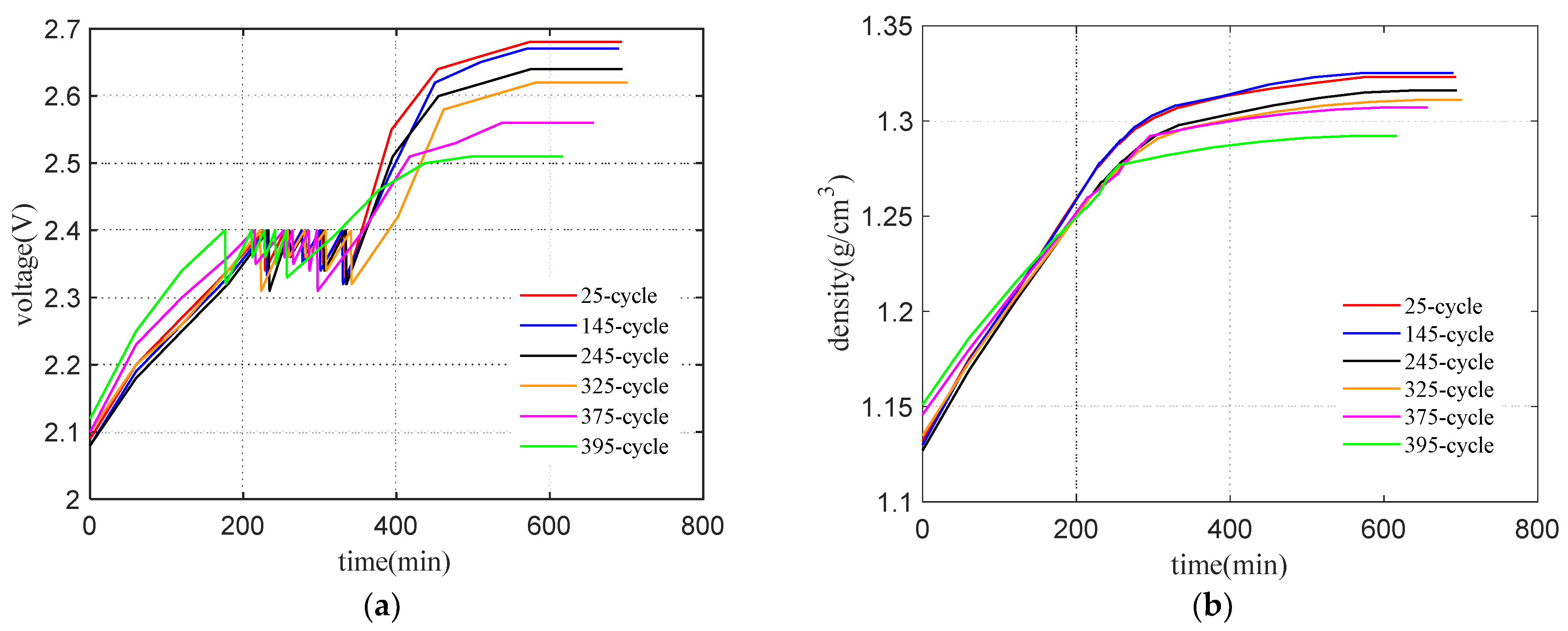
In the experiment, the change processes of the terminal voltage and electrolyte density during the charge process of the battery in different service cycles are as shown in Figure 3.
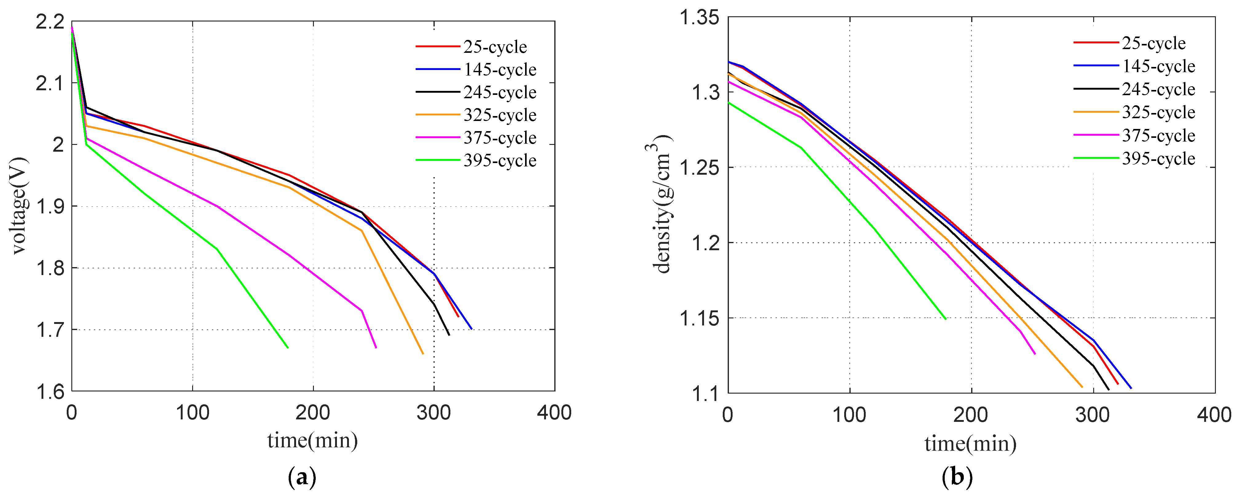
For the convenience of reference, the discharge processes of the battery under the 5 h discharge rate in different cycles are selected, and the change processes of its terminal voltage and electrolyte density are presented in Figure 4.
It can be seen that during the repeated use of the battery, under the same charge and discharge scheme, the terminal voltage, the electrolyte density, and other performances of the battery have changed significantly, indicating that the prediction model can track and adaptively adjust the battery state, which is very necessary for the accurate prediction of SOC.

4.2. Selection of Model Parameters

In this model, the parameters that need to be initialized mainly include: the activation function f in the OSELM algorithm for weak learning machine, the number of hidden layers h in OSELM, and the number of new samples p required for one update of the OSELM algorithm. In the improved AdaBoost algorithm process, the number of iterations is T, the ratio of the training samples for the weak learning machines to the total samples is g = N/m, the weight change coefficient is β , the error threshold is τ , and the maximum number of times of a single sample being extracted is k.
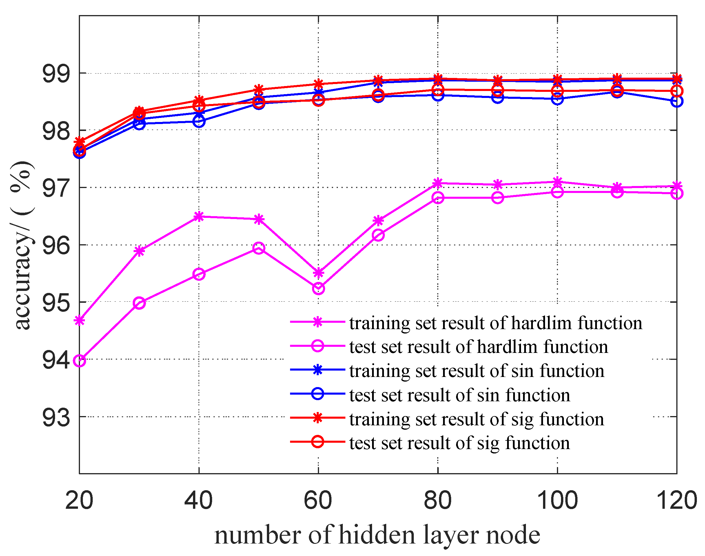
Firstly, the parameters for the activation function f in the OSELM algorithm and the number of hidden layers h in the OSELM are selected. The activation functions generally include the sig function, sin function, and hardlim function. The number of nodes at the hidden layer is within the range of [22,23], and the node number gradually increases by 10. The first 1800 samples of the 2216 samples are used as the training samples, and the remaining 416 samples are used as test samples. For the number p of new samples required by each update of the OSELM algorithm set as 1, the comparison of the prediction results under different values is shown in Figure 5:
It can be seen that when the sig function is used as the activation function, the obtained prediction results are the most optimal. When the number of nodes at the hidden layer is 80, the accuracies on both the training set and the test set reach the highest values without further increase. Then, as the number of nodes at the hidden layer continues to grow, it does not have a significant influence on the accuracy of the model, but the computational complexity is increased. Therefore, the sig function is used as the activation function for the OSELM model, and the number of nodes at the hidden layer is set as 80.
After determining the activation function f and the number of hidden layers h, the number p of new samples required for each update of the OSELM algorithm should be decided, assuming p is in the range of [1, 80], and p gradually increases by 10 nodes. The MAPE of the obtained test samples is shown in Table 1:
According to the results, when the value of p is 30, the accuracy of the prediction set is basically unchanged, while the computation time is reduced by nearly 50%, so the value of p is set as 30.
For the initial assignment of parameters in the AdaBoost algorithm, because there are many parameters, a random search algorithm is used as in [39,40,41]. With the MAPE of the predicted sample as the objective function, the constraint functions are: 3 ≤ T ≤ 20, the step size is 1; 0.001 ≤ τ ≤ 0.03, the step size is 0.005; 0.50 ≤ g ≤ 1, the step size is 0.05; 1.0 ≤ β ≤ 1.5, the step size is 0.1; 3 ≤ kT, the step size is 1.
The parameter values are finally determined as follows: the number of iterations T is 11, the error threshold τ is 0.01, the ratio g of the training samples for the weak learning machines to the total samples is 0.65, the weight change coefficient β is 1.2, and the maximum number of times k of a single sample being extracted is 8.

4.3. Verification of Effectiveness and Adaptability

4.3.1. Verification of Effectiveness

The 2216 samples collected during the battery experiment were divided. In the first case, the first 1800 samples were used as the training samples, and the remaining 416 groups were used as test samples. Then, the method proposed in this paper, the AdaBoost.R2-OSELM method, and the AdaBoost.R2-ELM method were used for prediction of these samples, and the results were compared. The activation function and the number of hidden layer nodes in the OSELM and ELM in each model are the same. Related parameters in the AdaBoost.R2 algorithm have the same values as those in the improved AdaBoost algorithm proposed in this paper.
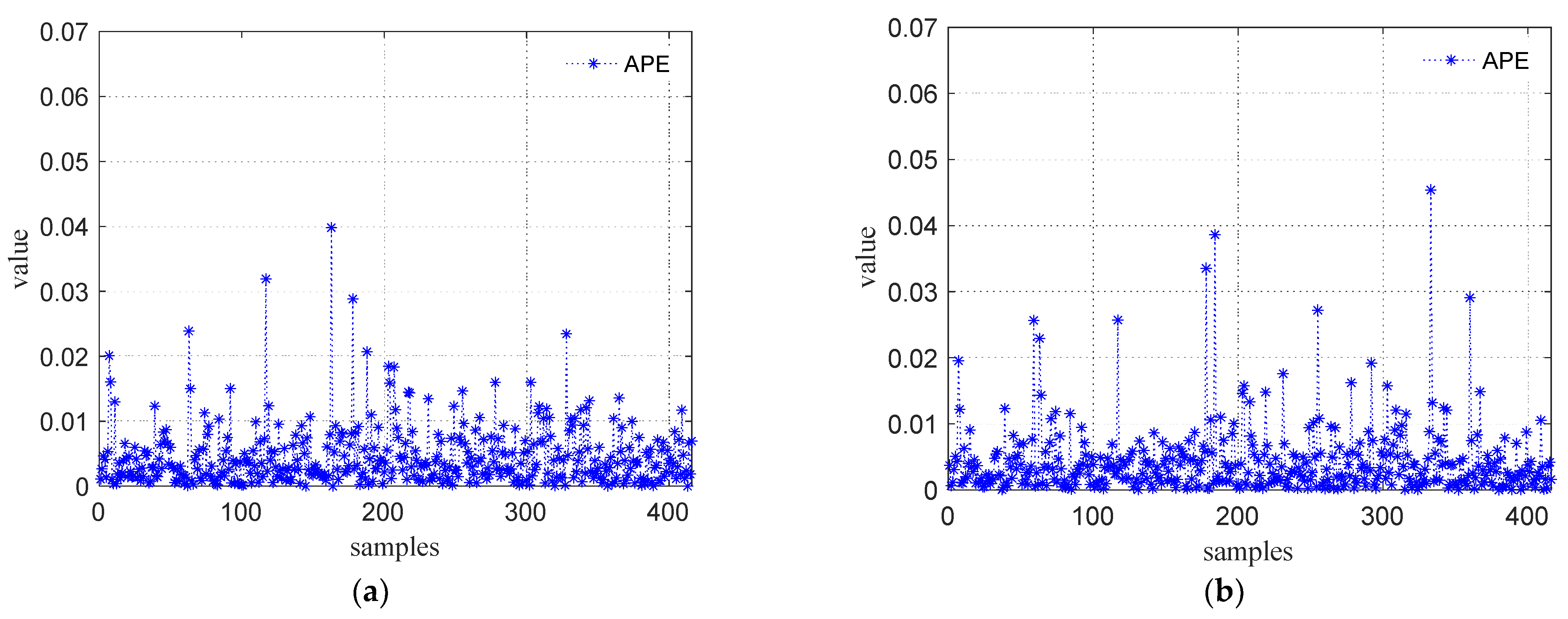
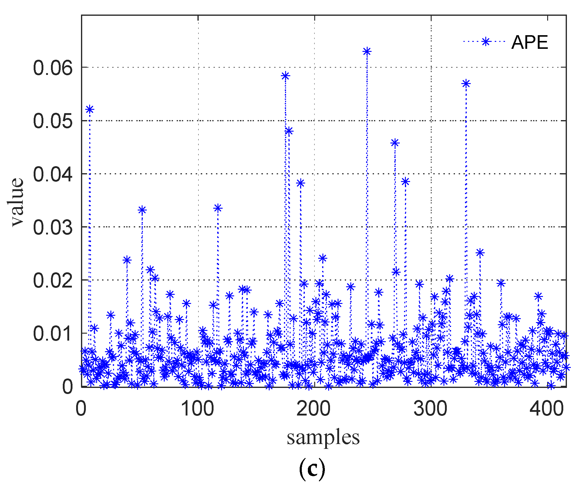
After training each neural network, the prediction results of the electrolyte density in the charge and discharge processes by using various network models were obtained, as shown in Figure 6, and the comparison of the prediction indicators is shown in Table 2, where AEmax refers to the maximum absolute error, and APEmax refers to the maximum relative error.
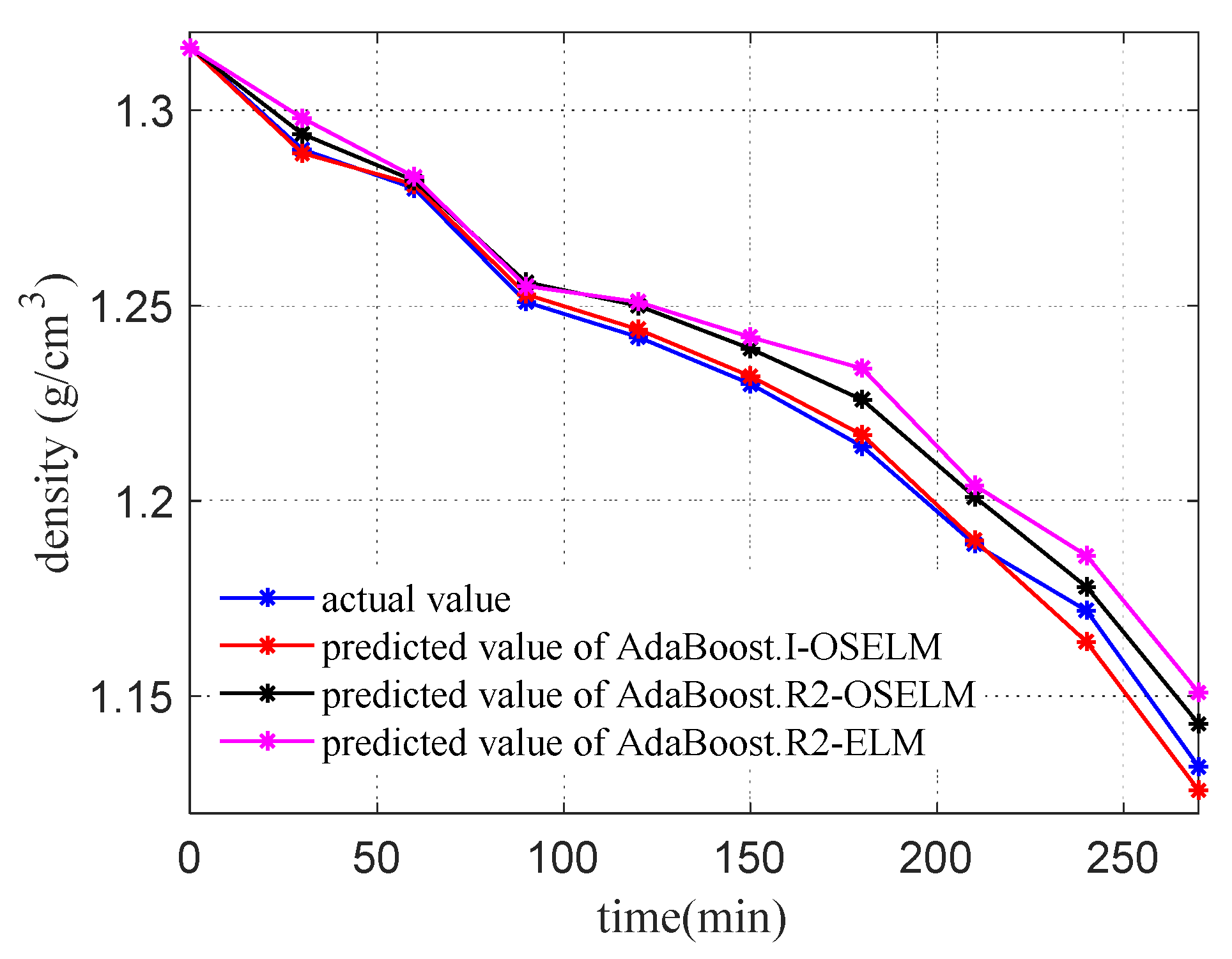
Intuitive comparison of the prediction results of density change for the predicted sample in the 366-th cycle during the variable current discharge process is made. The comparison between the prediction results using various models is shown in Figure 7.
In the first case of training, there were more training samples, but fewer test samples, that is, fewer samples for incremental learning. According to the prediction results, the three methods did not present significant difference in the overall prediction accuracy. Among them, the AdaBoost.I-OSELM model has the highest prediction accuracy. Compared with the AdaBoost.R2-OSELM model, the scores of the AdaBoost.I-OSELM model in the AEmax and APEmax indicators are 6.8% and 8.8% lower, which verifies the accuracy and effectiveness of the AdaBoost.I-OSELM method.

4.3.2. Verification of Adaptability

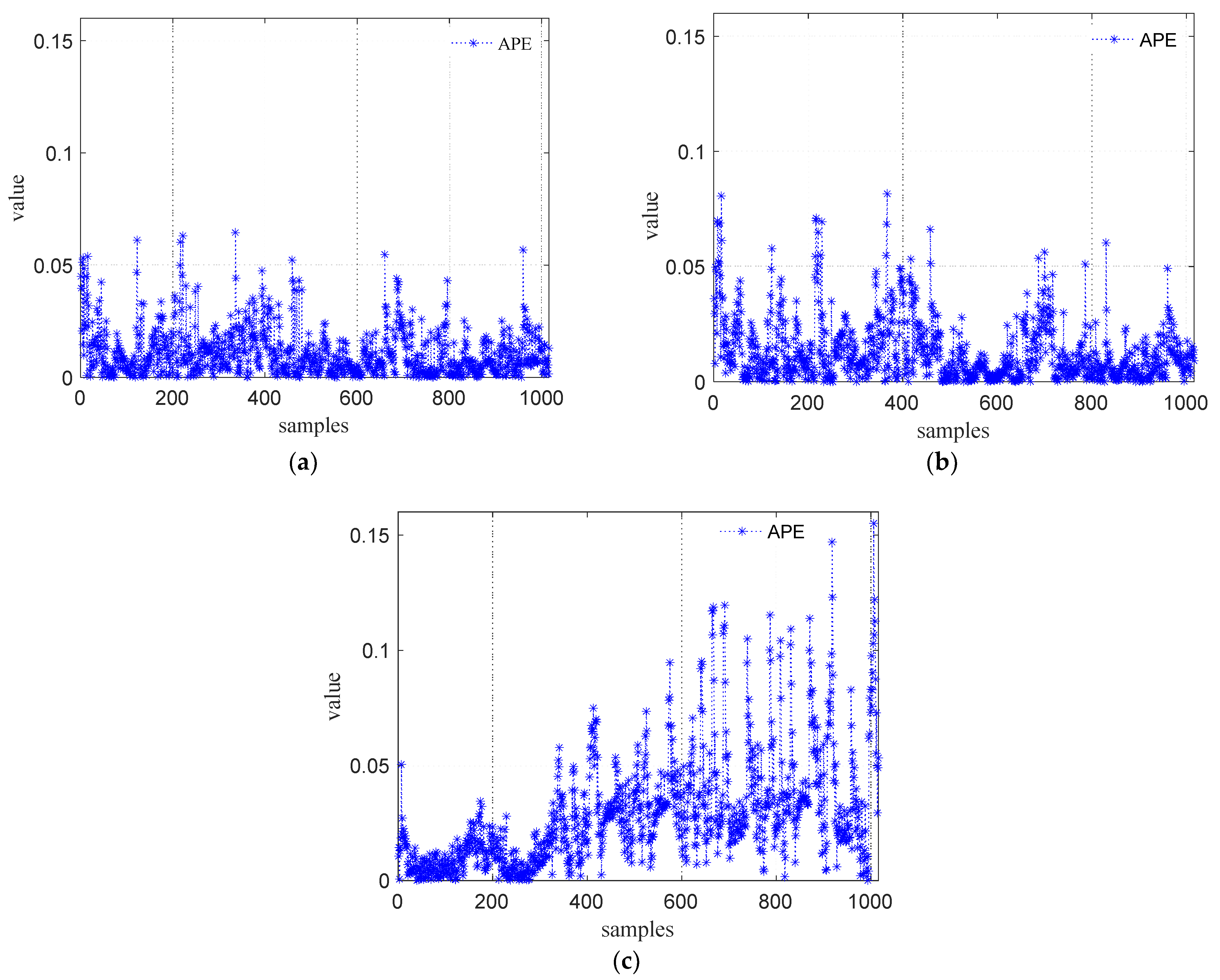
Still using the above three prediction models, in the second case, the first 1200 samples of the battery were used as the training samples, and the remaining 1016 samples were used as the test samples. The prediction results of the battery electrolyte density during the charge and discharge processes by using various models are demonstrated in Figure 8, and the comparison of related prediction indicators is shown in Table 3:
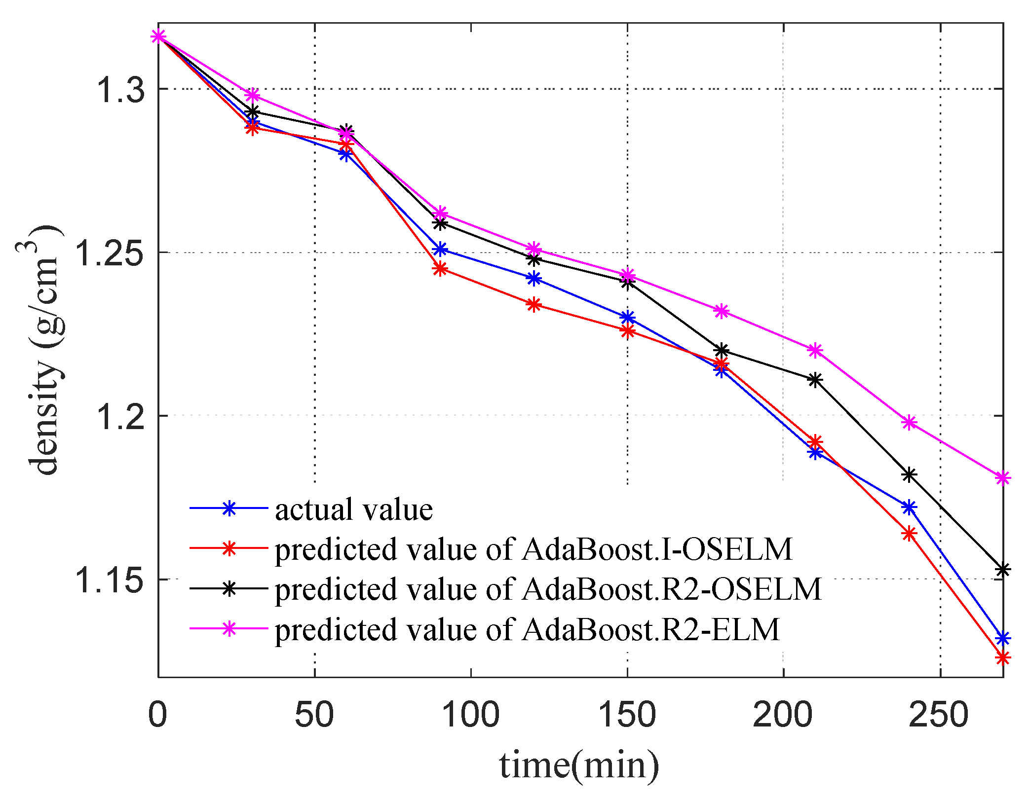
In this case, intuitive comparison is also made in terms of the prediction results of density change for the predicted sample in the 366th cycle during the variable current discharge process. The comparison between the prediction results using various models is shown in Figure 9:
In this case, there were many prediction samples, which can reflect the influence of the incremental learning ability of the model on the prediction accuracy. According to the prediction results, the AdaBoost.I-OSELM model and AdaBoost-OSELM model with the incremental learning ability significantly outperform the AdaBoost-ELM model without the incremental learning ability. Moreover, compared with the AdaBoost.R2-ELM model, the scores of the AdaBoost.R2-ELM model in the indicators of MAPE, MAE, and MSE are reduced by 75.4%, 58.3, and 84.2%, respectively. This is mainly because when the network continuously generates and acquires new samples, and when the model has the incremental learning ability, it can fully absorb and learn the newly acquired samples, and complete the tracking of changes in the system in a timely manner by dynamically adjusting the model parameters, so as to improve the prediction performance. Compared with the prediction results of the AdaBoost.R2-OSELM model, the AdaBoost.I-OSELM model has not only achieved higher overall prediction accuracy, but also effectively reduced the maximum absolute error and maximum percentage error of the model. Therefore, the adaptive ability of our method is further verified on the basis of the effectiveness and accuracy of model.

4.4. Comparison with Other Methods

To further verify the performance of the proposed method, it is compared with several commonly used data-driven methods which are both used for regression prediction on data [42], including the extreme learning machine (ELM), support vector machine (SVM), relevance vector machine (RVM), LSTM, BP neural network, and random forest (RF). Various algorithms are used to carry out battery SOC prediction for the test samples in the first and second cases discussed above, and the comparison results obtained are shown in Table 4 and Table 5:
According to the comparison results of the models, it can be concluded that for the first case with more training samples and fewer test samples, because various models had already carried out comprehensive learning and training of the system, they do not show significant difference in the prediction accuracy of test samples. Among various methods, our proposed method still maintains the best prediction accuracy, and the ELM method has the highest computational efficiency.
For the second case, that is, with more test samples, the training samples were limited to the working data of battery during the early and middle stages of its entire service life, which did not include the working data in the later stage of the battery. For algorithms without the incremental learning ability, it is difficult for them to track changes in the battery performance, so they generally have low prediction accuracy. In comparison, the algorithm proposed in this paper has the advantage of carrying out incremental learning of new samples for dynamic updates of the algorithm model, so that the model can maintain high prediction accuracy and has a strong adaptive ability, which reflects the superiority of our method.

5. Conclusions

The flooded large-capacity lead–acid battery investigated in this paper has broad applications in large electrical equipment as a power source, and accurate prediction of the SOC of this type of battery is very important for the management and use of the battery. In this paper, the AdaBoost.I-OSELM model is used to predict and study the battery SOC. According to the experiments and data verification, we can draw the following main conclusions:
1. The model has the incremental learning ability for new samples, and it can iteratively update the output weights of the model with less computation according to the newly acquired samples without repeatedly training the old samples. The incremental learning ability of the model is achieved, which has a high learning efficiency and strong adaptive ability. For the battery studied in this paper, when there were more prediction samples, the scores of our method in the prediction accuracy indicators of MAPE, MAE and MSE were reduced by 75.4%, 58.3, and 84.2%, respectively.
2. The prediction accuracy of the model can be further increased based on improvement of the traditional AdaBoost method, while reducing the maximum absolute error and the maximum relative error by 6.8% and 8.8%.
3. By comparing the prediction results of our method and other prediction methods, we can see that the model proposed in this paper achieved the highest prediction accuracy for battery SOC. Especially when there are a large number of prediction samples, the incremental learning ability of our method shows obvious advantages, which further verifies the accuracy and adaptability of the model.

Author Contributions

Conceptualization, S.S., W.C.; methodology, S.S., Z.Z.; software, Q.Z., Z.Y.; validation, J.S., Z.W. All authors have read and agreed to the published version of the manuscript.

Funding

Project supported by National Natural Science Foundation of China (52107063).

Conflicts of Interest

The authors declare no conflict of interest.

References

  1. Campillo-Robles, J.M.; Goonetilleke, D.; Soler, D.; Sharma, N.; Rodriguez, D.M.; Bucherl, T.; Makowska, M.; Turkilmaz, P.; Karahan, V. Monitoring lead-acid battery function using operando neutron radiography. J. Power Sources 2019, 438, 226976. [Google Scholar] [CrossRef]
  2. Luo, X.; Barreras, J.V.; Chambon, C.L.; Wu, B.; Batzelis, E. Hybridizing lead-acid batteries with supercapacitors: A methodology. Energies 2021, 14, 507. [Google Scholar] [CrossRef]
  3. Yong, J.Y.; Ramachandaramurthy, V.K.; Tan, K.M.; Mithulananthanb, N. A review on the state-of-the-arttechnologies of electric vehicle, its impacts and prospects. Renew. Sustain. Energy Rev. 2015, 49, 365–385. [Google Scholar] [CrossRef]
  4. Liu, J.W.; Wu, G.; Shi, C. Ampere hour integrated state of charge estimation method based on available capacity estimation and power increment curve. Instrum. Technol. 2021, 3, 33–37. [Google Scholar]
  5. Lashway, C.R.; Mohammed, O.A. Adaptive battery management and parameter estimation through physics-based modeling and experimental verification. IEEE Trans. Transp. Electrif. 2016, 2, 454–464. [Google Scholar] [CrossRef]
  6. Luo, Y.; Qi, P.; Huang, H.; Wang, J.; Wang, Y.; Li, P. Study on battery SOC estimation by ampere-hour integral method with capacity correction. Automot. Eng. 2020, 42, 681–687. [Google Scholar]
  7. Ping, S.; Ouyang, M.; Lu, L.; Li, J.; Feng, X. The co-estimation of state of charge, state of health, and state of function for lithium-ion batteries in electric vehicles. IEEE Trans. Veh. Technol. 2018, 67, 92–103. [Google Scholar]
  8. Yang, F.; Song, X.; Xu, F.; Tsui, K.L. State-of-charge estimation of lithium-ion batteries via long short-term memory network. IEEE Access 2019, 7, 53792–53799. [Google Scholar] [CrossRef]
  9. Guoliang, W.; Zhiyu, Z.; Daren, Y. Unsteady open circuit voltage method for state of charge estimation of electric vehicle batteries. Electr. Mach. Control. 2013, 17, 110–116. [Google Scholar]
  10. Yang, X.J.; Zhou, E.Z. Study of improved battery SOC estimation method. Chin. J. Power Sources 2016, 40, 1840–1844. [Google Scholar]
  11. Krivik, P.; Vaculik, S.; Baca, P.; Kazelle, J. Determination of state of charge of lead-acid battery by EIS. J. Energy Srorage 2019, 21, 581–585. [Google Scholar] [CrossRef]
  12. Ma, W.W.; Zheng, J.Y.; You, J.; Zhang, X.F. Kalman filter for estimating state-of-charge of VRLA batteries. Chin. Labat Man 2010, 47, 19–23. [Google Scholar]
  13. Pan, H.; Lü, Z.; Lin, W.; Li, J.; Chen, L. State of charge estimation of lithium-ion batteries using a grey extended Kalman filter and a novel open-circuit voltage model. Energy 2017, 138, 764–775. [Google Scholar] [CrossRef]
  14. Cui, W.H.; Wang, J.S.; Chen, Y.Y. Equivalent Circuit Model of Lead-acid Battery in Energy Storage Power Station and Its State-of-Charge Estimation Based on Extended Kalman Filtering Method. Eng. Lett. 2018, 26, 504–517. [Google Scholar]
  15. Shao, S.; Bi, J.; Yang, F.; Guan, W. On-line estimation of state-of-charge of Li-ion batteries in electric vehicle using the resampling particle filter. Transp. Res. Part D Transp. Environ. 2014, 32, 207–217. [Google Scholar] [CrossRef]
  16. Pola, D.A.; Navarrete, H.F.; Orchard, M.E.; Rabié, R.S.; Cerda, M.A.; Olivares, B.E.; Pérez, A. Particle-filtering-based discharge time prognosis for lithium-ion batteries with a statistical characterization of use profiles. IEEE Trans. Reliab. 2015, 64, 710–720. [Google Scholar] [CrossRef]
  17. Chen, Z.; Sun, H.; Dong, G.; Wei, J.; Wu, J.I. Particle filter-based state-of-charge estimation and remaining-dischargeable-time prediction method for lithium-ion batteries. J. Power Sources 2019, 414, 158–166. [Google Scholar] [CrossRef]
  18. Yang, F.; Li, W.; Li, C.; Miao, Q. State-of-charge estimation of lithium-ion batteries based on gated recurrent neural network. Energy 2019, 175, 66–75. [Google Scholar] [CrossRef]
  19. Li, C.; Xiao, F.; Fan, Y. An approach to state of charge estimation of lithium-ion batteries based on recurrent neural networks with gated recurrent unit. Energies 2019, 12, 1592. [Google Scholar] [CrossRef]
  20. Xia, K.G.; Qian, X.Z.; Yu, Y.H.; Zhang, J.Y. Accurate estimation of charge state of lithium battery based on BP neural network. Electron. Des. Eng. 2019, 27, 61–65. [Google Scholar]
  21. Lipu, M.S.H.; Hannan, M.A.; Hussain, A.; Saad, M.H.; Ayob, A.; Uddin, M.N. Extreme learning machine model for state-of-charge estimation of lithium-ion battery using gravitational search algorithm. IEEE Trans. Ind. Appl. 2019, 55, 4225–4234. [Google Scholar] [CrossRef]
  22. Li, R.; Xu, S.; Li, S.; Zhou, Y.; Zhou, K.; Liu, X.; Yao, J. State of charge prediction algorithm of lithium-ion battery based on PSO-SVR cross validation. IEEE Access 2020, 8, 10234–10242. [Google Scholar] [CrossRef]
  23. Wu, Z.Q.; Shang, M.Y.; Shen, D.D.; QI, S.Q. Prediction of SOC of lead-acid battery in pure electric vehicle based on BSA-RELM. J. Renew. Sustain. Energy 2018, 10, 054103. [Google Scholar] [CrossRef]
  24. Li, X.J.; Zhao, J.H.; Yang, J.B.; Zhang, J.T. Research on the charge model of lead-acid batteries onboard modern submarines. Ship Sci. Technol. 2011, 33, 58–61. [Google Scholar]
  25. Zhang, Y.; Yu, Y.; Zhang, B.; Zhao, J.; Xu, W.; Zhou, Q. Overview of the current situation and development of lead-acid battery. Chin. Labat Man 2021, 58, 27–31. [Google Scholar]
  26. Han, Y.B. Life cycle comparative study of lithium batteries and lead-acid batteries. Chin. Labat Man 2014, 51, 186–189. [Google Scholar]
  27. Wu, H.B.; Gu, X.; Zhao, B.; Zhu, C.Z. Comparison study on model and state of charge estimation of typical battery. J. Electron. Meas. Instrum. 2014, 28, 717–723. [Google Scholar]
  28. Liu, B.; Bi, X.X.; Dang, J.P.; Liu, Q.; Wang, J. Degradation trend prediction of battery in substation based on support vectorregression. J. Power Supply 2020, 18, 207–214. [Google Scholar]
  29. Galar, M.; Fernandez, A.; Barrenechea, E.; Bustince, H.; Herrera, F. A review on ensembles for the class imbalance problem: Bagging, boosting, and hybrid-based approaches. IEEE Trans. Syst. Man Cybern. Part C 2012, 42, 463–484. [Google Scholar] [CrossRef]
  30. Wang, Y.W.; Feng, L.Z. Improved AdaBoost algorithm using group degree and membership degree based noise detection and dynamic feature selction. J. ZheJiang Univ. 2021, 55, 367–376. [Google Scholar]
  31. Huang, G.B.; Zhu, Q.Y.; Siew, C.K. Extreme learning machine: Theory and applications. Neurocomputing 2006, 70, 489–501. [Google Scholar] [CrossRef]
  32. Liang, N.Y.; Huang, G.B.; Saratchandran, P.; Sundararajan, N. A fast and accurate online sequential learning algorithm for feedforward networks. IEEE Trans. Neural Netw. 2006, 17, 1411–1423. [Google Scholar] [CrossRef] [PubMed]
  33. Zhang, R.; Lan, Y.; Huang, G.B.; Xu, Z.B. Universal approximation of extreme learning machine with adaptive growth of hidden nodes. IEEE Trans. Neural Netw. Learn. Syst. 2012, 23, 365–371. [Google Scholar] [CrossRef] [PubMed]
  34. Nie, Q.; Jin, L.; Fei, S.; Ma, J. Neural network for multi-class classification by boosting composite stumps. Neurocomputing 2015, 149, 949–956. [Google Scholar] [CrossRef]
  35. Li, L.; Wang, C.; Li, W.; Chen, J. Hyperspectral image classification by AdaBoost weighted composite kernel extreme learning machines. Neurocomputing 2018, 275, 1725–1733. [Google Scholar] [CrossRef]
  36. Freund, Y.; Schapire, R.E. A decision-theoretic generalization of online learning and all application to boosting. J. Comput. Syst. Sci. 1997, 55, 119–139. [Google Scholar] [CrossRef]
  37. Schapire, R.E.; Singer, Y. Improved boosting algorithms using confidence-rated predictions. Mach. Learn. 1999, 37, 297–336. [Google Scholar] [CrossRef]
  38. Reddy, T.B. Linden’s Handbook of Batteries, 4th ed.; McGraw-Hill Education: New York, NY, USA, 2010. [Google Scholar]
  39. Bergstra, J.; Bengio, Y. Random search for hype parameter optimization. J. Mach. Learn. Res. 2012, 13, 281–305. [Google Scholar]
  40. Chen, W.; Chen, J.X.; Jiang, Y.Q.; Song, D.L.; Zhang, W.D. Fault identification of rolling bearing based on RS-LSTM. China Sci. Pap. 2018, 13, 1134–1140. [Google Scholar]
  41. Ma, L.Y.; Yu, S.L.; Zhao, S.Y.; Sun, J.M. Superheated steam temperature prediction models based on XGBoost optimized with random search algorithm. J. North China Electr. Power Univ. 2021, 48, 99–105. [Google Scholar]
  42. How, D.; Hannan, M.A.; Lipu, M.; Ker, P.J. State of charge estimation for lithium-ion batteries using model-based and data-driven methods: A review. IEEE Access 2019, 7, 136116–136136. [Google Scholar] [CrossRef]
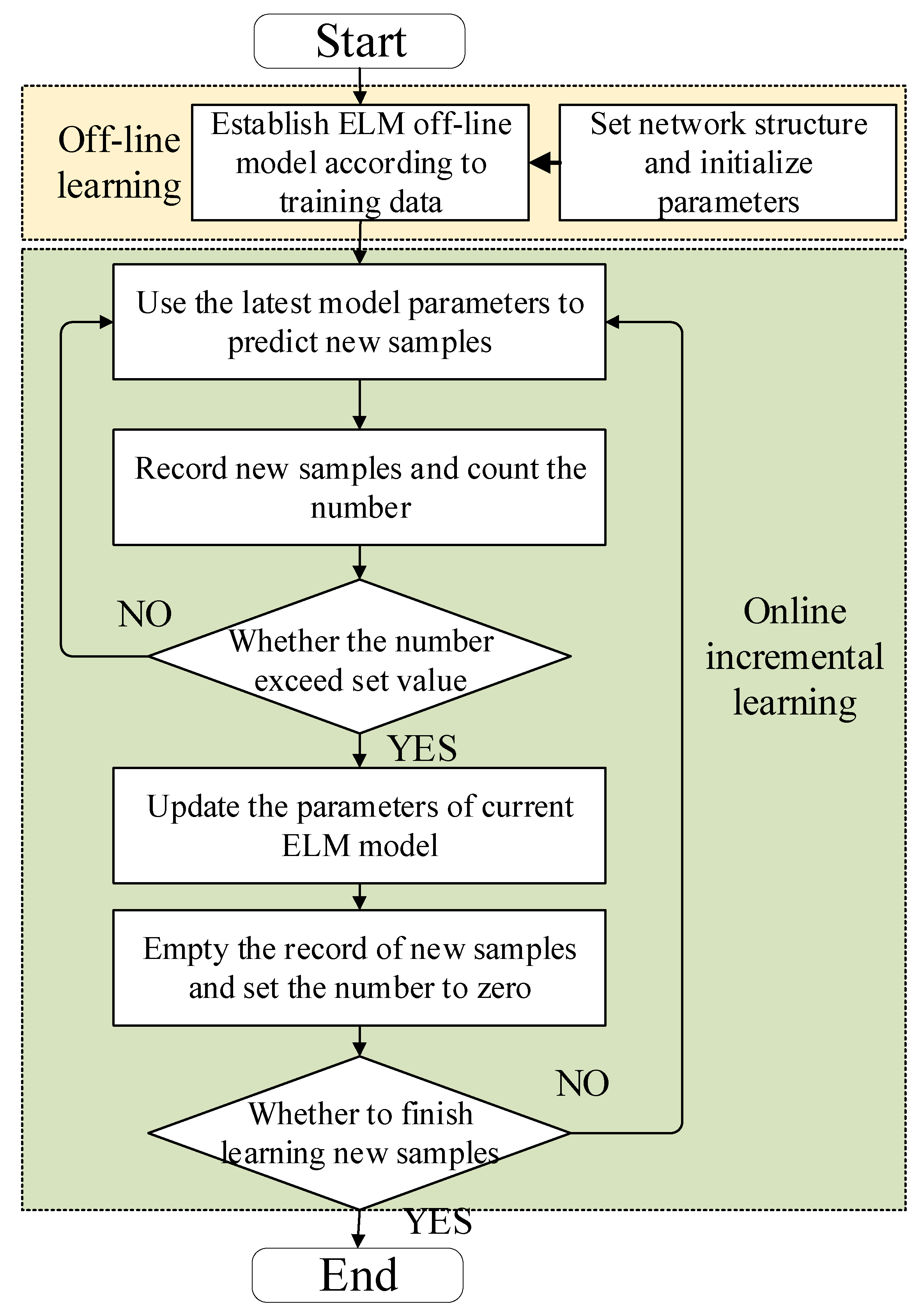
Figure 1. Prediction process of OSELM model.
Energies 15 05842 g001
Figure 2. Prediction process of battery SOC by AdaBoost.I-OSELM model.
Energies 15 05842 g002
Figure 3. Comparison of charging process in different cycles. (a) Variation of terminal voltage. (b) Variation of the electrolyte density.
Energies 15 05842 g003
Figure 4. Comparison of discharging process in different cycles. (a) Variation of terminal voltage. (b) Variation of the electrolyte density.
Energies 15 05842 g004
Figure 5. Prediction accuracy under different activation functions and hidden layer nodes.
Energies 15 05842 g005
Figure 6. Prediction results of different models in the first case. (a) AdaBoost.I-OSELM model. (b) AdaBoost.R2-OSELM model. (c) AdaBoost.R2-ELM model.
Energies 15 05842 g006aEnergies 15 05842 g006b
Figure 7. Prediction of discharge process density for 366 cycles by different models in the first case.
Energies 15 05842 g007
Figure 8. Prediction results of different models in the second case. (a) AdaBoost.I-OSELM model. (b) AdaBoost.R2-OSELM model. (c) AdaBoost.R2-ELM model.
Energies 15 05842 g008
Figure 9. Prediction of discharge process density for 366 cycles by different models in the second case.
Energies 15 05842 g009
Table 1. Prediction accuracy under different values of p.
p11020304050607080
Accuracy (%)98.9198.8998.9198.9098.5298.4398.3998.4090.38
Time (s)0.2410.1650.1410.1260.1190.1120.1090.1070.106
Table 2. The prediction indexes of different neural networks in the first case.
ModelAdaBoost.R2-ELM AdaBoost.R2-OSELMAdaBoost.I-OSELM
MAPE0.00980.00750.0062
MAE0.01290.00980.0084
MSE4.54 × 10−43.50 × 10−43.22 × 10−4
AEmax0.10260.07120.0663
APEmax0.06300.04450.0406
Table 3. The prediction indexes of different neural networks in the second case.
ModelAdaBoost R2-ELM AdaBoost R2-OSELMAdaBoost.I-OSELM
MAPE0.04150.01450.0102
MAE0.04920.01760.0205
MSE0.00570.00110.0009
AEmax0.17620.08630.0693
APEmax0.15500.08160.0645
Table 4. The prediction of different models in the first case.
AlgorithmELM SVMLSTMRFBPAdaBoost.I-OSELM
MAPE0.01020.00960.01210.00740.01040.0062
MAE0.01320.01230.01560.00930.01340.0084
MSE4.78 × 10−43.66 × 10−45.25 × 10−43.41 × 10−44.29 × 10−43.22 × 10⁻⁴
AEmax0.10360.08740.12030.06690.08390.0663
APEmax0.08530.06710.10220.04360.06350.0406
Time/s0.0020.0710.1990.1020.0160.021
Table 5. The prediction of different models in the second case.
AlgorithmELM SVMLSTMRFBPAdaBoost.I-OSELM
MAPE0.04610.04330.05210.03880.04460.0102
MAE0.05220.05010.05980.04260.05150.0205
MSE0.00680.00620.00790.00480.00630.0009
AEmax0.23010.21310.31250.11320.19230.0693
APEmax0.21050.19220.28630.09010.16250.0645
Time/s0.0030.2330.920.5240.0660.082
Publisher’s Note: MDPI stays neutral with regard to jurisdictional claims in published maps and institutional affiliations.