Application of the ARMA Model to Describe and Forecast the Flotation Feed Solids Flow Rate

Abstract

The flow rate of solids is subject to random disturbances of the changing feed and can significantly affect the quantitative and qualitative parameters of the coal flotation products. This quantity can be described as a stochastic process. The paper presents the results of the solids flow rate model for coal flotation identification calculations, treated as a disturbance to the process. This is an innovative approach to modelling those quantitative parameters of the flotation feed that are measurably available and whose random changes have a significant impact on the enhancement process under industrial conditions. These include the volumetric flow rate of the feed and, in particular, concentration of solids in the feed. Therefore, it is suggested that random changes of these two parameters of the feed should be mapped using a model of one quantity—the flow rate of solids. This solution is advantageous because this quantity, as a quantitative parameter of the feed, has a significant impact on the course of the coal flotation process. The model is necessary in the process of designing an automatic control system through simulation tests. It allows us to generate a data string simulating random changes to this quantitative parameter of the feed. On this basis, in the simulation model, the correct functioning of the automatic control system is tested, the task of which is to compensate the influence of this disturbance. To determine the empirical model of the feed solids flow rate, measurement data obtained during the registration of the solids concentration and volumetric flow rate of the feed were used in four consecutive periods of operation of an industrial facility of one of the Polish coal processing plants. The time courses of the solids flow rate in the feed were described by ARMA (autoregressive–moving-average model) means, and the two-stage least squares method was used to estimate the model parameters. The results of the identification and verification of the designated model showed the correctness of adopting the third-order ARMA model, with parameters a₁ = −1.0682, a₂ = −0.2931, a₃ = 0.3807, c₁ = −0.1588, c₂ = −0.2301, c₃ = 0.1037, and variance σ²_ε = 0.0891, white noise sequence ε_t, determined on the basis of a series of residuals described by the fifth-order model. It has been shown that the identified model of the flow rate of solids of the feed to flotation as disturbances can be used to develop a predictive model that allows forecasting the modelled quantity with a prediction horizon equal to the sampling period. One-step forecasting based on the determined predictor equation was found to give results consistent with the recorded values of the solid part flow rate of the feed and the extreme values of the prediction error are within the range from −1.08 to 2.90 kg/s.

1. Introduction

The change in time of the flotation feed solids flow is a random disturbance that can be described as a stochastic process. Therefore, it is important to describe the properties of this process by using a model. The lack of such studies in relation to the industrial process prompted the authors to take up this issue, the more so that the model of the flotation feed solids flow is necessary for the next stage of research, i.e., to develop the structure of automatic control of the flotation process with compensation of disturbances in the form of changes in the flow of flotation feed solids flow.

Flotation is a physicochemical enhancement process and is of interest to many scientists [1,2,3,4,5,6]. In the case of hard coal, enhancing coal with the flotation method is used for the feed consisting of grains smaller than 0.5 mm [7,8,9,10]. It is a very complex process and difficult to control [11,12]. 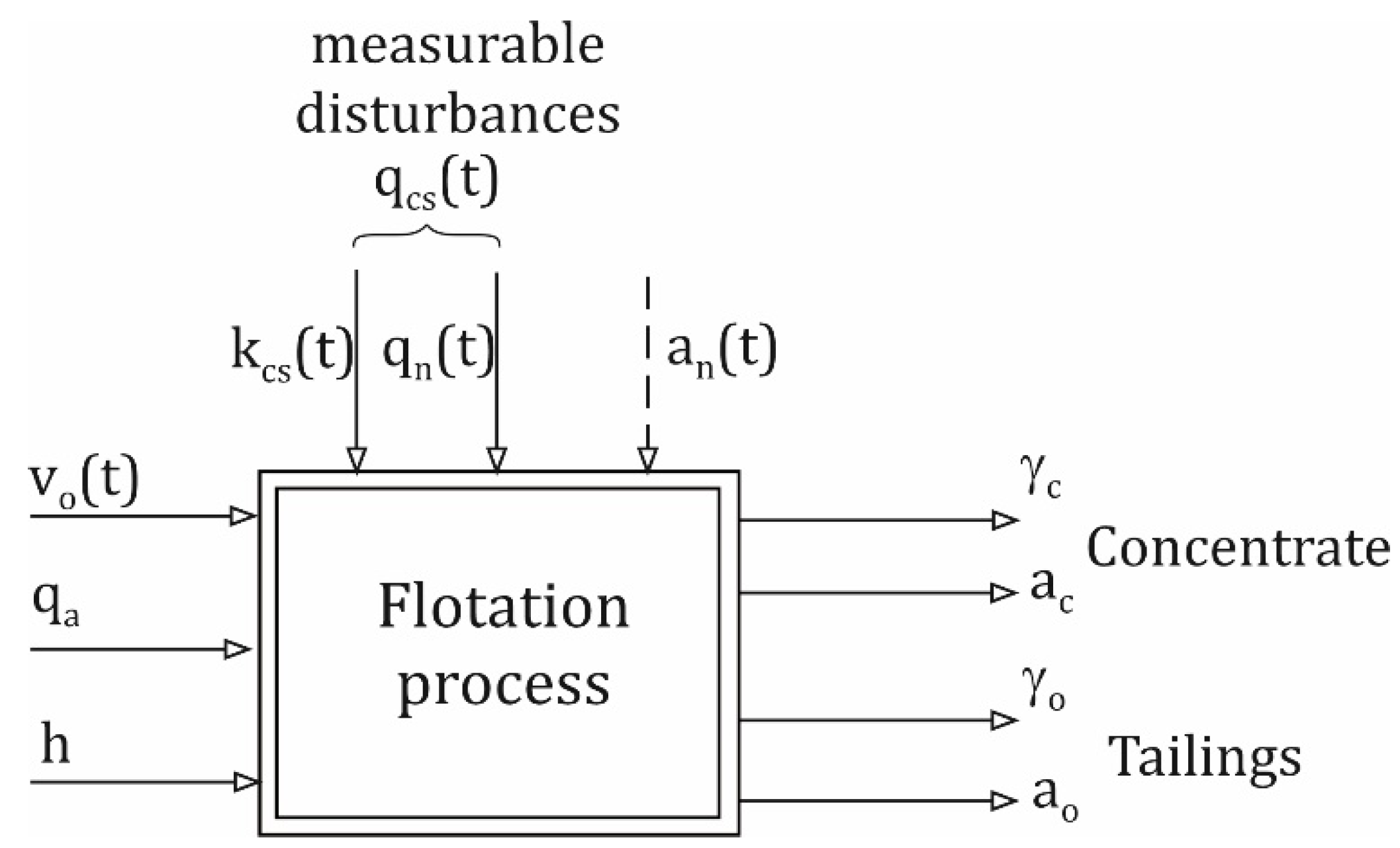For this reason, this process is the subject of extensive scientific research [3,13,14,15,16,17,18], including modelling of this process [19,20,21,22,23,24,25,26]. The basic input quantities for the flotation process are: feed flow rate-q_n with ash content a_n and concentration of solids in the feed k_cs, flotation reagent flow rate v_o, air flow rate for aeration q_a, and the level of suspension in the flotation cell h. The output quantities are: concentrate output γ_k, ash content in the concentrate a_k, waste output γ_o, and the ash content of the waste a_o (Figure 1).

Coal flotation feedstock is characterised by a number of parameters, and the control strategy often depends on their changes [27,28]. An important parameter is the solids flow rate, which is subject to random disturbances of the changing feed and should be treated as a disturbance in the automatic control system of the flotation process. Changes in solids flow rate significantly affect the flotation effect as changes in the values of quantitative and qualitative product parameters [29]. Therefore, in the flotation process control systems, the dosage of the flotation reagent should depend on the current value of the feed quantity parameters. One way is the constant dosage control of the flotation reagent, where the amount of reagent is fed into the system in proportion to the solids flow rate:

$$v_o\left(t\right)=d_o\times q_{cs}\left(t\right)$$

(1)

where: d_o is the flotation reagent dosage, m³/kg, and q_cs is the flow of solids of the feedstock for flotation, kg/s. Of the feed quantity parameters, the solids concentration and the flow rate are measurable. Therefore, the value of the solids flow can be determined from the relation:

$$q_{cs}\left(t\right)=k_{cs}\left(t\right)\times q_n\left(t\right)$$

(2)

where: k_cs is the solid concentration, kg/m³, and q_n is the flotation feed flow rate, m³/s.

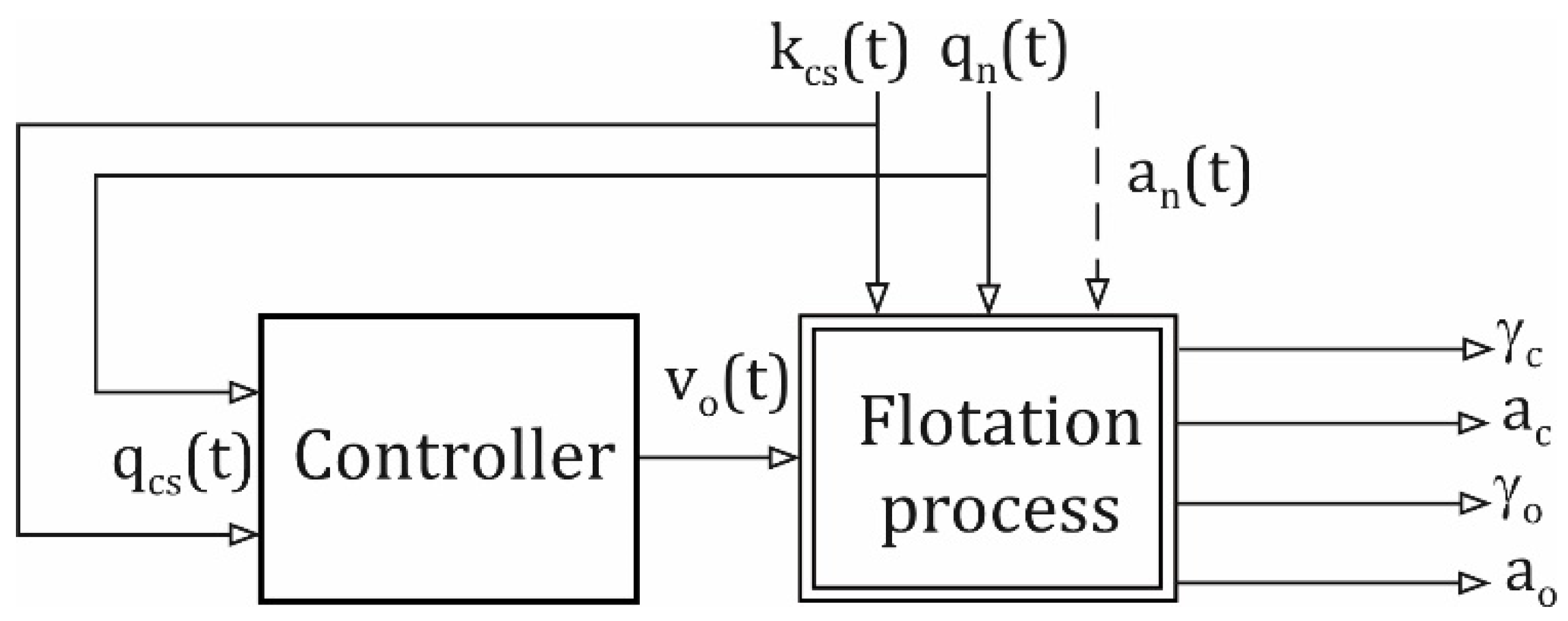
Figure 2 shows a flow chart of the control with a constant dose of flotation reagent. It is a form of automatic control in an open system with compensation of disturbance, which is the flow rate of solids of the feedstock. It should be noted that in addition to the flotation reagent dosing control system, industrial systems use local loops for automatic stabilisation of the suspended solids level in the flotation cell and the aeration air flow rate.

Computer-aided engineering focused on the use of simulation models can be used to improve enrichment technology [30,31,32]. In the case of coal flotation, modelling can be carried out on the basis of object identification in order to represent its dynamic and static properties as accurately as possible. The aim of such research comes down to the development of a mathematical model of the object and then its numerical form, i.e., a simulation model. In the flotation process, input signals in the form of quantitative and qualitative parameters of the changing feed can be treated as disturbing signals. Modelling of these disturbances should be considered in a cognitive aspect, but they are important from the point of view of selecting appropriate technical measures to conduct the process in a way that compensates for their impact, especially in systems of automatic control of this process. The issue of modelling the parameters of the coal flotation feed takes on particular importance in the case of industrial processes whose feed, for technological reasons, is characterised by significant fluctuations of the solids flow rate and its high values, the reduction of which is difficult to implement without incurring large financial outlays. A random disturbance in the form of time variations of the flow rate of the feed solids can be represented as a stochastic process, for the description of which ARMA models can be used. These models are widely used in the description of stochastic processes, including those related to the processing of nonferrous ores [33].

ARMA (autoregressive–moving-average model) and ARIMA (autoregressive–integrated-moving-average model) models are very often used to forecast various stochastic processes [34,35,36,37,38]. They can be used to predict the value of the feed solids flow rate. Prediction models of this quantity can be used in the design of automatic control systems (predictive control). In the case of systems where manual control of the coal flotation process is used, information about future values of the solids flow rate in the feed can be useful for decision-making by operators and process experts, in terms of changes in the settings of control signals such as the dosage of the flotation reagent.

The paper presents the problem of modelling the flow rate of solids in the flotation feed, based on empirical data recorded in a Polish coal preparation plant. The ARMA model, determined by the double least squares method, was used for their description. On the basis of the flow of feed solids model as a disturbance in coal flotation, the predictor equation for this stochastic process was determined, which enables one-step forecasting.

2. Parameter Estimation Method for ARMA Models

To determine the mathematical model of the feed solids flow rate for the flotation process q_ks, a model with discrete transmittance expressed by the equation was adopted:

$$y_t=K\left(z^{-1}\right)\times e_t=\frac{C\left(z^{-1}\right)}{A\left(z^{-1}\right)}\times e_t$$

(3)

where: e_t is a sequence of uncorrelated disturbances with mean equal to zero and variance ${\sigma }_e^2$, and y_t is a concentrated sequence of recorded values of the solids flow rate of the flotation feed with the number of samples N, kg/s.

The current value of the process described by the ARMA model with Equation (3) is a linear combination of past moment outputs and filtered white noise. Many methods are known to identify ARMA models. These include the methods described in previous studies [39,40,41]. For the parameter estimation of the ARMA model with Equation (3), the two-stage least squares method given by Durbin was used [42]. The algorithm first involves determining a sequence of residuals ε_t, which is an approximation of the unknown white noise sequence e_t:

$$e_t\approx {\epsilon }_t=B\left(z^{-1}\right)\times y_t$$

(4)

The relation between Equations (3) and (4) is expressed by the equation:

$$B\left(z^{-1}\right)=\frac{A\left(z^{-1}\right)}{C\left(z^{-1}\right)}=1+b_1{z}^{-1}+\dots +b_p{z}^{-p}$$

(5)

To determine the order of p of the model (4) and the values of the parameters b₁, b₂,…, b_p, it is necessary to determine a sequence of residuals ε_t. Fitting a model of the autoregressive process (4) of order p to the signal sequence y_t is to determine the parameters b₁, b₂,…, b_p, minimising the value of the criterion J_b expressed by Equation (6).

$$J_b={\displaystyle \sum }_{t=p+1}^N{\left(B\left(z^{-1}\right)\times y_t\right)}^2$$

(6)

The order p of the model (4) is determined with the indicator FPE(p) (Final Prediction Error) defined as [43]:

$$FPE\left(p\right)=\frac{N+p}{N-p}\times {\sigma }_{\epsilon }^2\left(p\right)$$

(7)

The criterion FPE(p) depends on the variance of the residuals expressed by the following equation:

$${\sigma }_{\epsilon }^2\left(p\right)=\frac{1}{N-p}{\displaystyle \sum }_{t=p+1}^N{\left(y_t+b_1{y}_{t-1}+\dots +b_p{y}_{t-p}\right)}^2$$

(8)

The order of the model (4) is defined for the minimum criterion value (7). For the criterion adopted with the use of the FPE order p, the autoregression model AR(p) the values of the parameters b₁, b₂,…, b_p are calculated and then the sequence of ε_t residuals is determined, according to the Equation (4). The sequence ε_t is then used to fit the ARMA model to the measured series of data y_t. This operation leads to the estimation of parameters a₁, a₂, …, a_n and c₁, c₂, …, c_n ARMA model the order n (n < p) described with Equation (9) with values such that the minimum reaches the criterion value:

$$J_{ac}={\displaystyle \sum }_{t=p+1}^N{\left(A\left(z^{-1}\right)\times y_t-C\left(z^{-1}\right)\times {\epsilon }_t\right)}^2$$

(9)

where $A\left(z^{-1}\right)=1+a_1{z}^{-1}+\dots +a_n{z}^{-n}$ $C\left(z^{-1}\right)=1+c_1{z}^{-1}+\dots +c_n{z}^{-n}$.

In order to determine the order of the ARMA model with Equation (3), the ε_t sequence of residuals is checked, expressed by the equation:

$${\epsilon }_t=y_t+a_1{y}_{t-1}+a_2{y}_{t-2}+\dots +a_n{y}_{t-n}-c_1{\epsilon }_{t-1}-c_2{\epsilon }_{t-2}-\dots -c_n{\epsilon }_{t-n}$$

(10)

The sequence of residuals (10) should have the characteristics of a white noise sequence, which is assessed by analysing the autocorrelation function of the sequence under test ε_t. The autocorrelation function is expressed by the following equation:

$$R_{\epsilon }\left(k\right)=\frac{1}{N}{\displaystyle \sum }_{t=k+1}^N{\epsilon }_t\times {\epsilon }_{t-k}$$

(11)

Its normalized form is described by the following equation:

$${\rho }_{\epsilon }\left(k\right)=\frac{R_{\epsilon }\left(k\right)}{R_{\epsilon }\left(0\right)}$$

(12)

A useful test for determining the order n of an ARMA model is to examine the residual variance of the model, determined according to:

$${\sigma }_{\epsilon }^2=\frac{1}{N-n-1}{\displaystyle \sum }_{t=n+1}^N{\left({\epsilon }_t\right)}^2$$

(13)

Variance (13) is calculated from the sequence of residuals described by Equation (10). Its value decreases slightly for subsequent orders of the stochastic process estimated model, larger than the proper order n. Therefore, the order of model (3) is taken to be that order n for which the corresponding value of the residual variance, determined according to Equation (13), is slightly larger than the value of the variance calculated for models of higher orders and significantly smaller than those of lower orders.

3. Prediction Model for a Stochastic Process

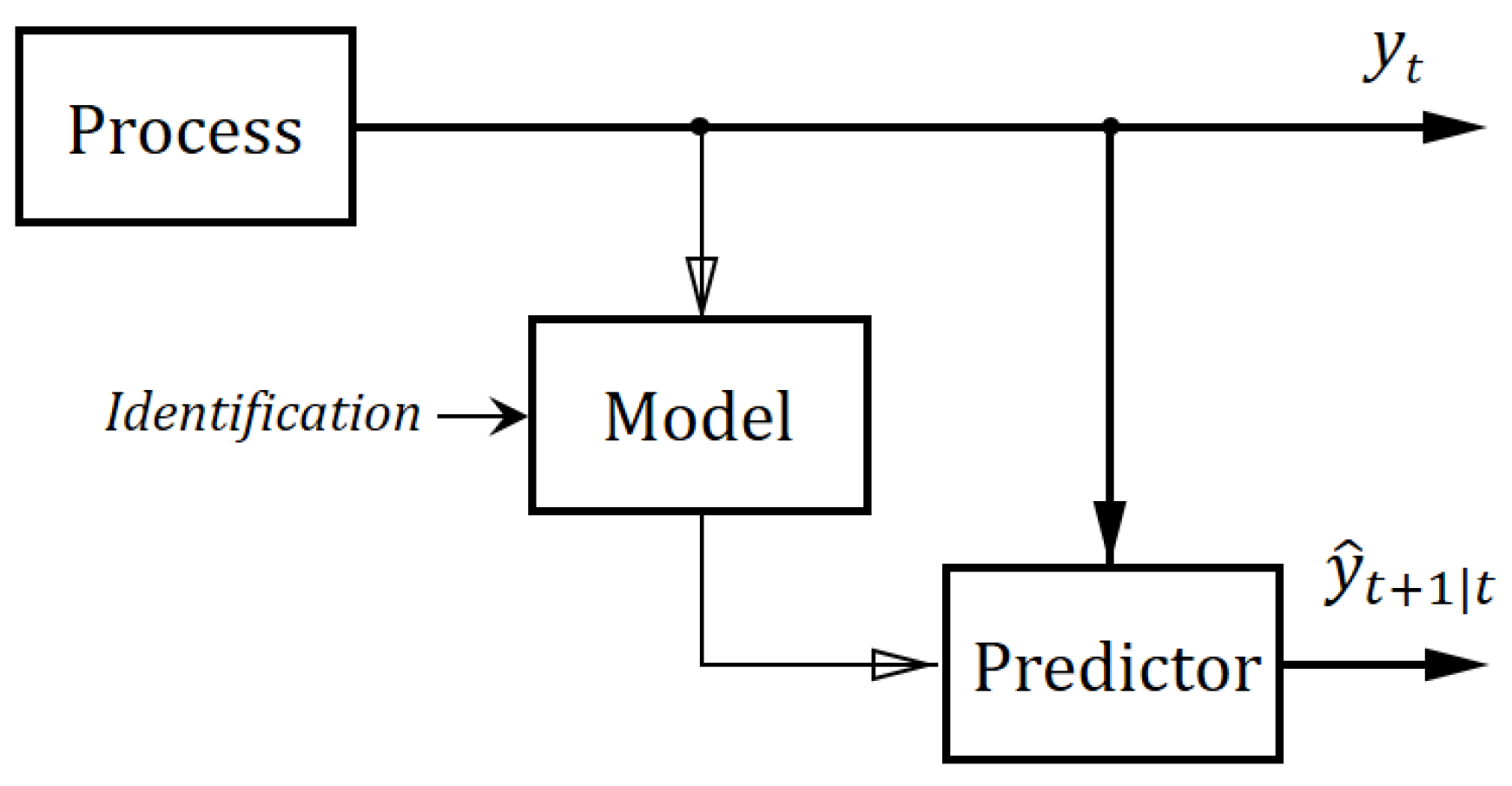
The method of determining the equation for predicting the time series y can be presented in a simplified manner using a flow chart as in Figure 3. The determination of the predictor equation for a stochastic process is performed in the following steps.

-

Recording of measured data y_t,

-

Identification of the process model of Equation (3) with the use of the two-stage least squares method,

-

Using the determined parameters of the model (3) in the predictor equation.

It is easy to notice that the essential step in developing a predictor for a stochastic process, according to Figure 1, is the identification of the model of Equation (3). In the case under consideration, this step is the same as using the process model identification method, which is described in Section 2.

According to the adopted process model (3), the value of the quantity observed at t time is described by the equation:

$$y_t=-a_1{y}_{t-1}-a_2{y}_{t-2}-\dots -a_n{y}_{t-n}+e_t+c_1{e}_{t-1}+c_2{e}_{t-2}+\dots +c_n{e}_{t-n}$$

(14)

From Equation (15) it follows that at the time (t + 1) the value of the measured quantity under consideration can be represented by the equation:

$$y_{t+1}=-a_1{y}_t-a_2{y}_{t-1}-\dots -a_n{y}_{t-n-1}+e_{t+1}+c_1{e}_t+c_2{e}_{t-1}+\dots +c_n{e}_{t-n+1}$$

(15)

Assuming the designation ${\widehat{y}}_{t+1|t}$ as the signal forecast value y at the time (t + 1), worked at the time t and by subtracting this value from both sides of the Equation (15) it is obtained:

$$y_{t+1}-{\widehat{y}}_{t+1|t}=\left(-a_1{y}_t-a_2{y}_{t-1}-\dots -a_n{y}_{t-n-1}+c_1{e}_t+c_2{e}_{t-1}+\dots +c_n{e}_{t-n+1}-{\widehat{y}}_{t+1|t}\right)+e_{t+1}$$

(16)

Because the difference between the value of a signal and its prediction is the prediction error, this can be described by the equation

$$e_t=y_t-{\widehat{y}}_{t|t-1}$$

(17)

Equation (16) can be transformed into:

$${\widehat{y}}_{t+1|t}=-a_1{y}_t-a_2{y}_{t-1}-\dots -a_n{y}_{t-n-1}+c_1{e}_t+c_2{e}_{t-1}+\dots +c_n{e}_{t-n+1}$$

(18)

The time series equation is then obtained with the prediction horizon equal to the sampling period. In the case of a stochastic process, Equation (18) enables one-step forecasting of the observed (measured) quantity.

4. Results of the Flotation Feed Solids Flow Rate Model Identification

4.1. Test Conditions

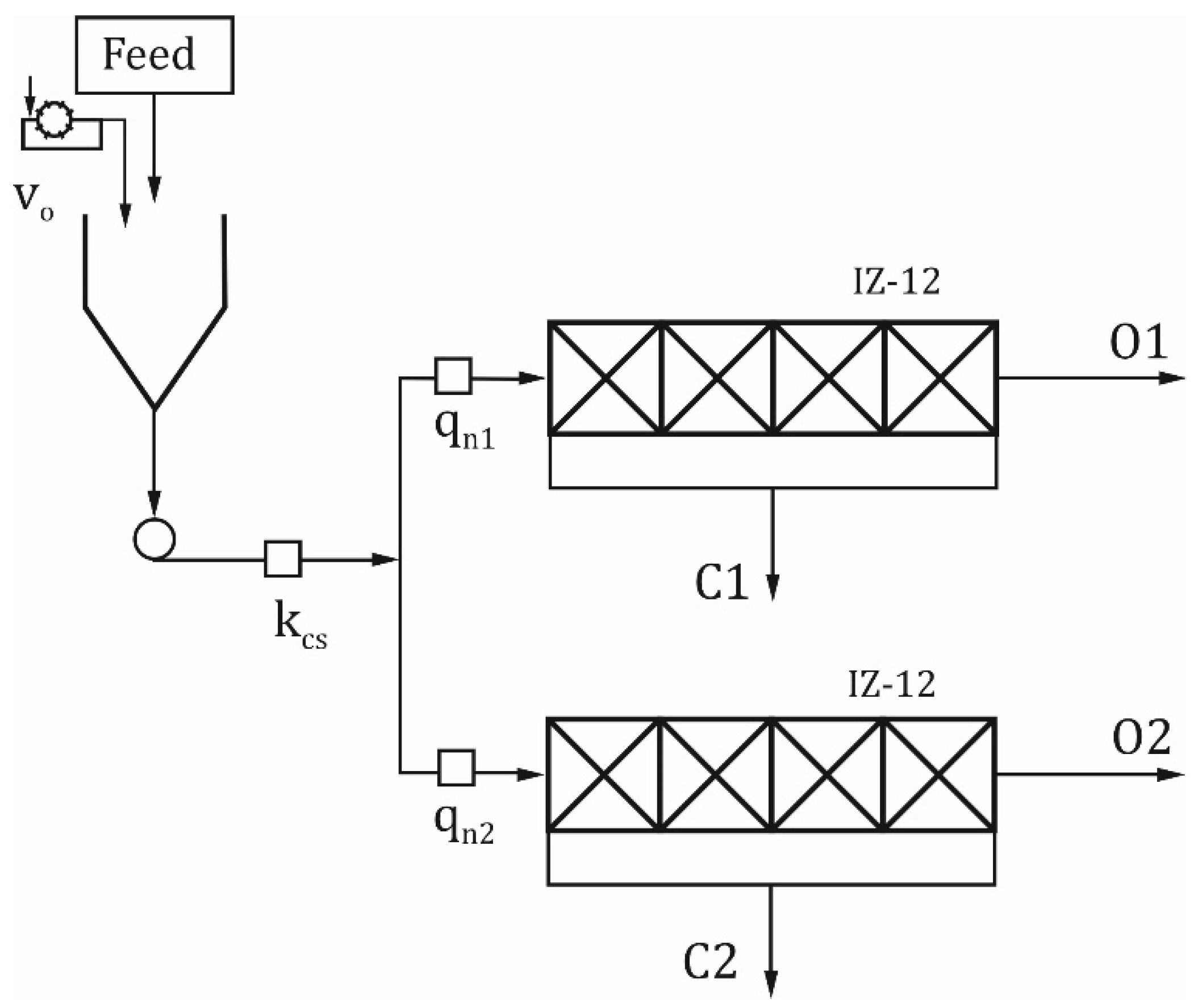
Identification was carried out based on data recorded during four consecutive, continuous (without breaks) periods of operation of IZ-12 flotation machines, installed in one of the Polish coal processing plants. A diagram of an industrial flotation facility is shown in Figure 4.

In the industrial facility, the feed for flotation (steam coal) came from radial thickeners. The outlets of these thickeners, which are the source of the flotation feed, were combined in a tank and fed to the process. The flotation feed obtained in this way was directed to two IZ-12 type flotation machines working in parallel. The waste from these flotation machines was directed to the next IZ-12 flotation machine for secondary enhancement. This configuration was a result of the flotation feed high density. The feed flow rate to the flotation machines was measured using Danfoss electromagnetic flow meters, whereas the solids concentration was measured using a POLON radiometric densitometer. The radiometric density meter used works on the principle of gamma radiation absorption. It is equipped with a radiation source in the form of the ¹³⁷Cs cesium isotope [44,45]. Data were recorded with a sampling period T_s equal to 60 s using an industrial computer. The instantaneous flow values of the flotation feed solids for previously recorded measurement data from flow meters and densimeter were determined from the equation:

$$y\left[i\right]=k_{cs}\left[i\right]\times \left(q_{n1}\left[i\right]+q_{n2}\left[i\right]\right)$$

(19)

where k_cs is the concentration of solids in the coal flotation feed, kg/m³ q_n1 is the feed flow rate to the flotation tank 1, m³/s, q_n2 is the feed flow rate to the flotation tank 2, m³/s, and I is the sampling step, i = t/T_s.

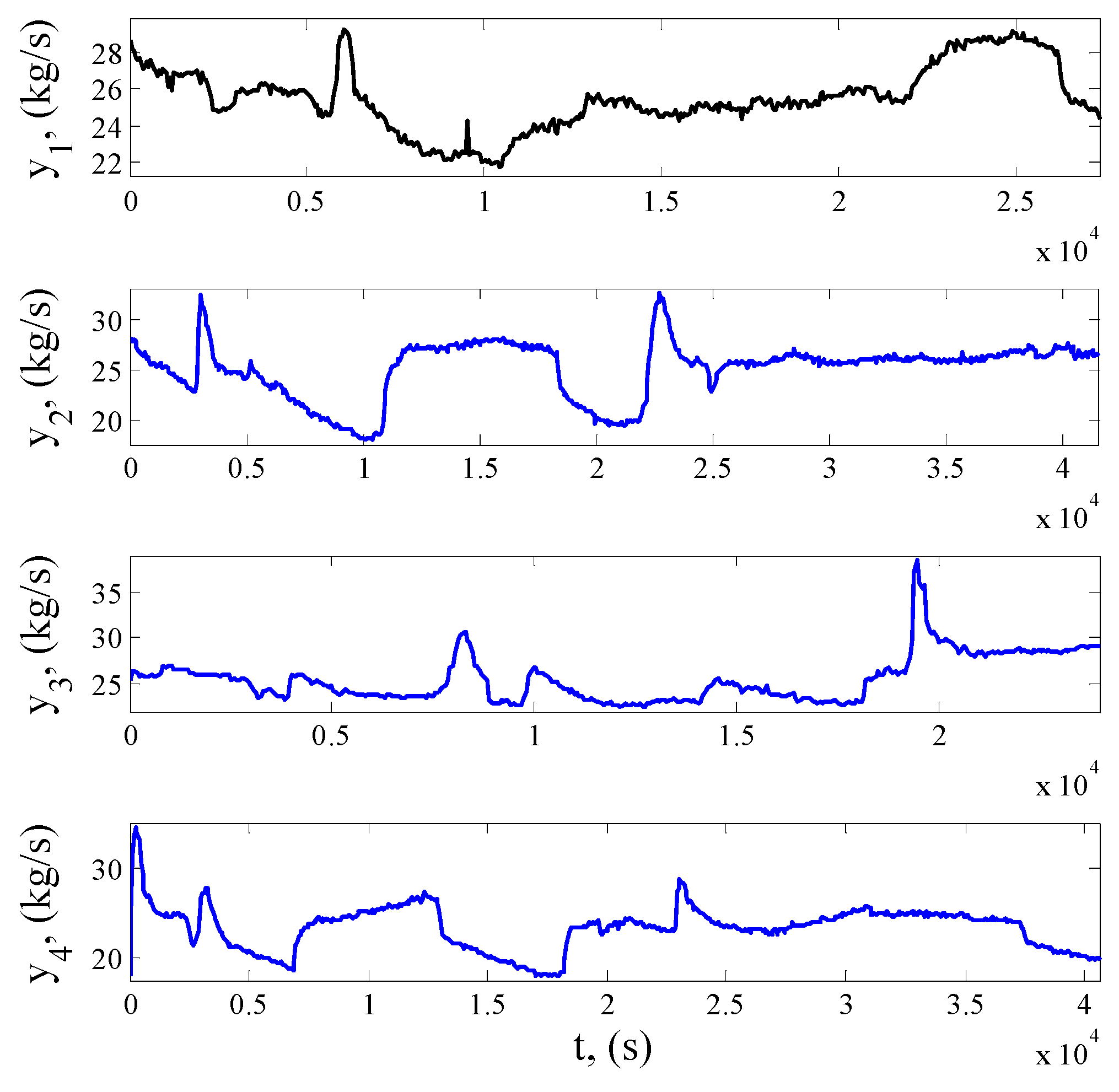
The condition for the correctness of the experiment was to obtain four continuous, significantly long (several hours), consecutive periods of the process operation. The industrial experiment conducted produced four data series for the individual measured quantities, the observed range of change of which is summarised in

Table 1. The range of variations of solids flow rate, solids contraction, and feed flow rate to the flotation process.

Data Series	y (kg/s)		kcs (kg/m3)		qn1 10−2 (m3/s)		qn2 10−2 (m3/s)
	Min	Max	Min	Max	Min	Max	Min	Max
1	21.69	29.31	173.55	228.99	62.96	69.96	58.12	67.16
2	18.06	32.60	146.12	247.45	61.13	73.62	52.75	66.88
3	22.46	38.51	177.11	235.28	54.44	97.61	51.51	77.25
4	17.97	34.63	144.01	253.27	62.50	72.07	52.61	67.43

. The data series relating to the solids flow rate are denoted as: y₁, y₂, y₃, and y₄. Their time courses are presented in Figure 5. The lengths of the individual data series are 457, 694, 400, and 678 points, respectively, so they cover long periods of the flotation industrial facility operation, that is, 7 h and 37 min, 11 h and 34 min, 6 h and 40 min, and 11 h and 18 min, respectively. As the values summarised in Table 1 and the time courses in Figure 5 show, the observed range of variation in the flow rate of the feed solids shows a significant range of instantaneous values. As part of the conducted identification research, the first series of empirical data (y₁) was used to determine the order and model parameters with the structure (3). The remaining three series were used to verify the determined model.

4.2. Results of the Flotation Feed Solids Flow Rate Model Identification as a Disturbance of the Flotation Process

According to the algorithm described in Section 2, the FPE criterion was used to determine the order p of the model (4). Estimation of the parameters of Equation (4) up to and including the 16th order was performed. Based on the calculations made, it was found that for the first series of data (y₁) the optimum in terms of criterion (7) is the order p = 5, whereas for the other series it was 3 or 4. Therefore, the estimation of the parameters of model (3) was carried out from order n = 1 to n = p−1, for two values of the model residual sequence: p = 4 and p = 5, assuming an appropriate starting point. The identification task was carried out for the first series of measurement data, and the results obtained are summarized in

Table 2. Flow rate model parameters of coal flotation feed solids with structure (3) estimated for the first series of measured data.

The Sequence of Residuals	p = 4			p = 5
	b1 = −0.9179, b2 = −0.2076, b3 = 0.03973, b4 = 0.1047			b1 = −0.9057, b2 = −0.2023, b3 = 0.0143, b4 = −0.0020, b5 = 0.1168
ARMA Model	n			n
	1	2	3	1	2	3	4
a1	−0.9857	−1.3718	−0.9436	−0.9861	−1.5158	−1.1259	−0.7749
a2	-	0.3848	−0.1663	-	0.5264	−0.2679	−0.4207
a3	-	-	0.1301	-	-	0.4068	0.0561
a4	-	-	-	-	-	-	0.1627
c1	−0.0678	−0.4515	−0.0240	−0.0802	−0.6106	−0.2200	0.1285
c2	-	0.1759	0.0192	-	0.1761	−0.2653	−0.1004
c3	-	-	0.1014	-	-	0.1081	−0.0224
c4	-	-		-	-	-	0.1227

.

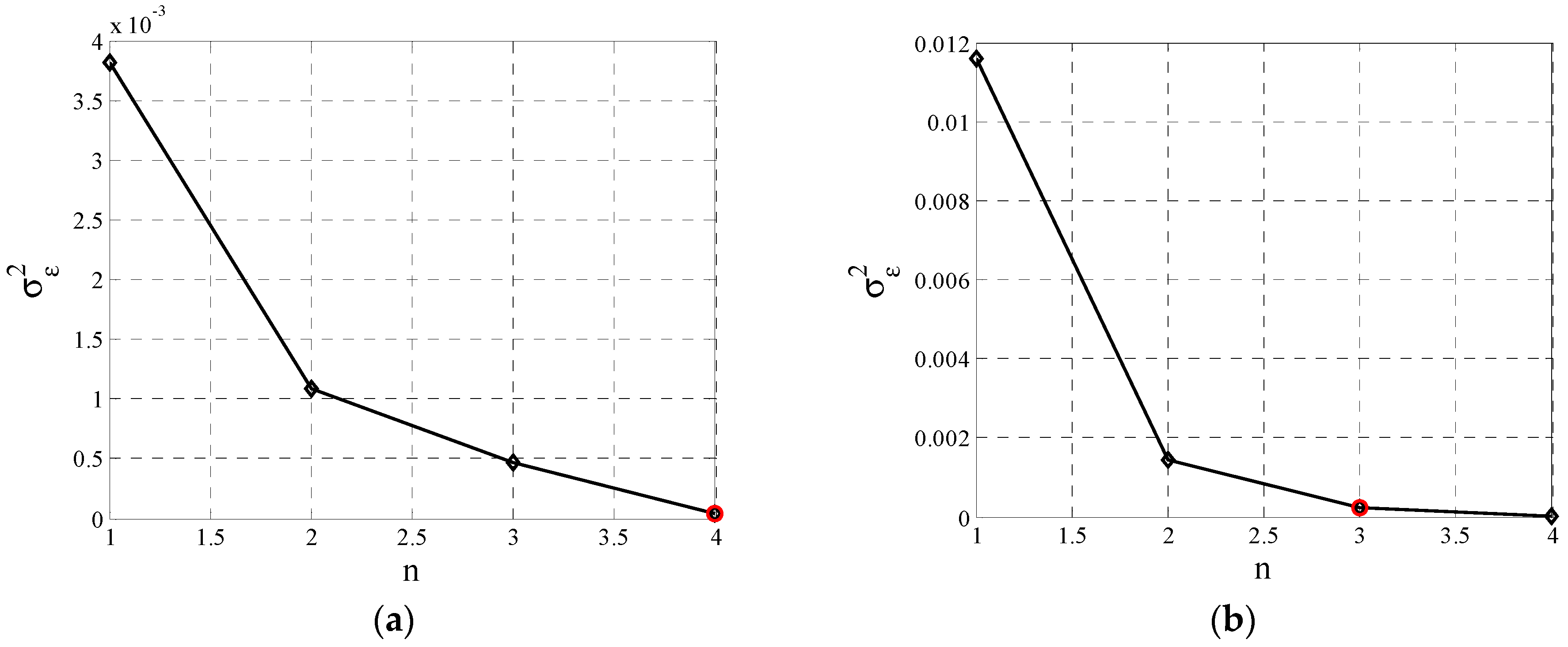
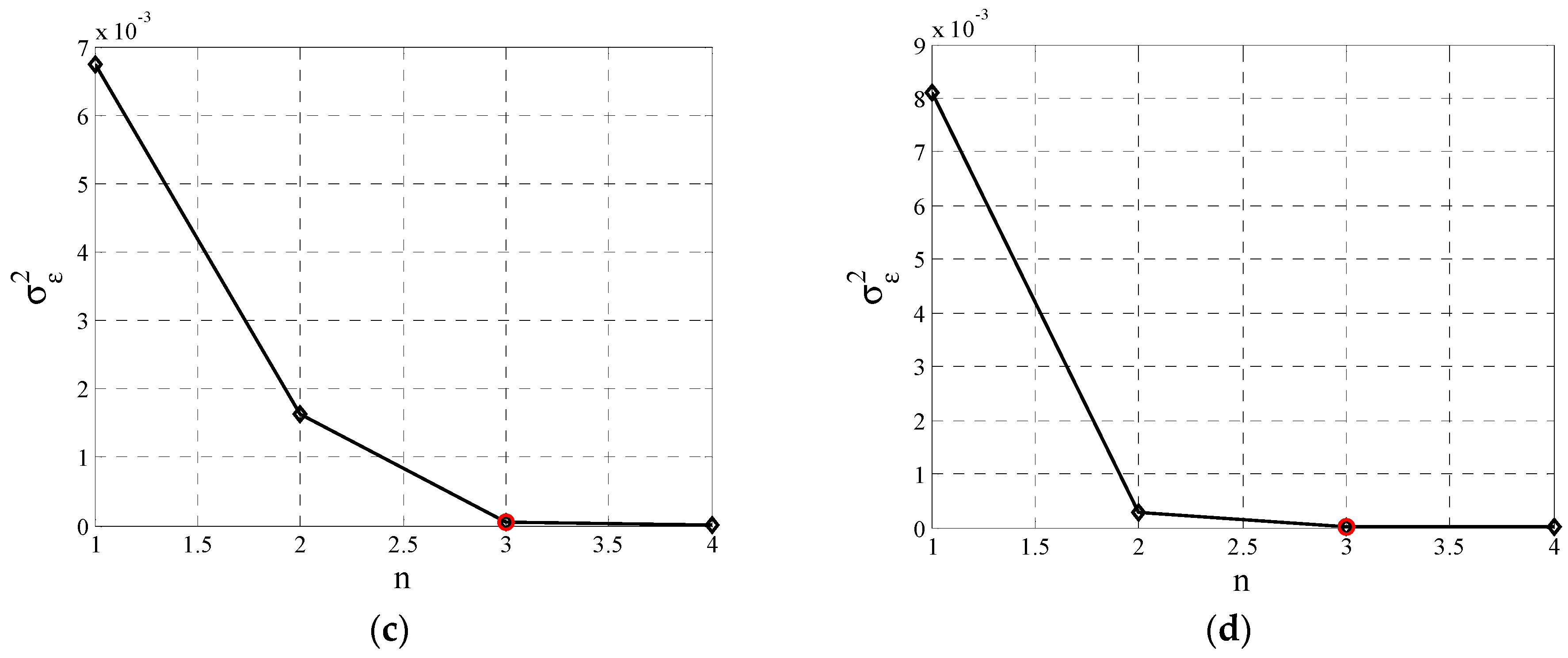
The dependence of the criterion (13) on the ARMA model order determined for all measured data series is presented in Figure 6, and the results in the form of estimated parameters of third-order ARMA models for the remaining empirical data series are summarised in

Table 3. Parameters of third-order ARMA models estimated for successive series of measured data.

Model Parameters	Series of Measured Data
	1	2	3	4
a1	−1.1259	−1.1413	−1.5472	−1.1428
a2	−0.2679	−0.3258	0.6563	−0.1290
a3	0.4069	0.4808	−0.0794	0.2877
c1	−0.2200	0.1249	−0.2510	0.0600
c2	−0.2653	−0.3256	−0.0428	−0.1059
c3	0.1081	−0.0908	0.1066	−0.0027

.

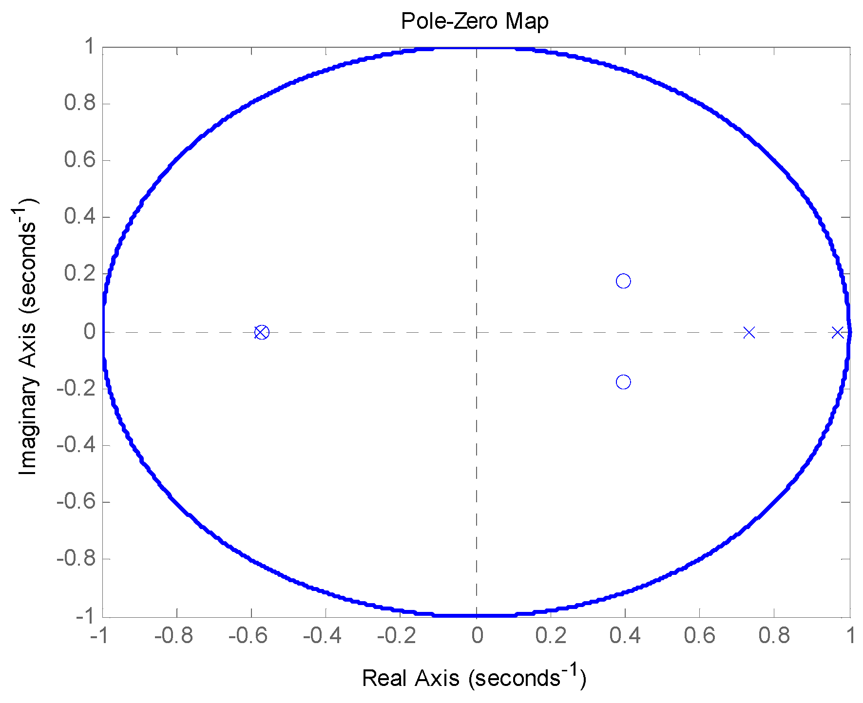
Based on the test results obtained, which are presented graphically in Figure 6, a model of the third order with parameters was determined for the first series of measured data with values equal to:

$$a_1=-1.1259, a_2=-0.2697, a_3=0.4068, c_1=-0.2200, c_2=-0.2653, c_3=0.1081$$

(20)

Based on the positions of zeros and poles in relation to the unit circle, it can be concluded that a model with a structure of (3) and parameters (20) is stable (Figure 7).

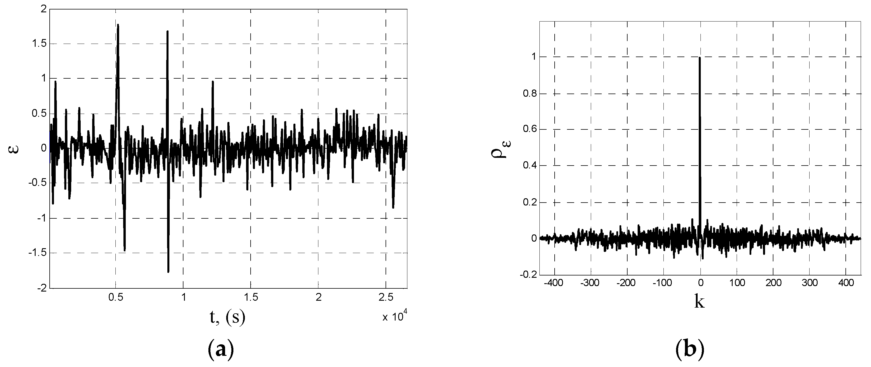
In a further evaluation of the ARMA model with parameters (20), its residuals were examined. The residuals of the model and the autocorrelation function of the residuals are shown graphically in Figure 8.

To generalise the interference model, 10 time courses of the feed solids flow rate were generated using the ARMA model with parameters (20) when the model is stimulated by a random variable with normal distribution, mean value equal to zero and variance σ²_ε = 0.0891, white noise sequence ε_t. The time courses were simulated using a sampling period of 60 s and the length of the data sequences was 550 samples, approximately equal to the average length of the recorded signals. Example simulations of the feed solids flow rate are shown in Figure 9.

Based on the data sequences generated in this way, the identification of the third-order ARMA model parameters was carried out separately for each of the courses. The results obtained are presented in

Table 4. Identification results of solids flow models into the feed determined from 10 simulated time courses.

Model Parameters	No. of Model Identified on the Basis of a Simulated Course										Average Values	σij
	1	2	3	4	5	6	7	8	9	10
a1	−1.1485	−1.0727	−1.0305	−0.9490	−1.5122	−1.0755	−0.9738	−0.9274	−0.9115	−1.0811	−1.07	0.17
a2	0.0098	−0.3540	−0.3268	−0.4537	0.5216	−0.2676	−0.6644	−0.4694	−0.6110	−0.3155	−0.29	0.34
a3	0.1612	0.4380	0.3875	0.4341	0.0136	0.3542	0.6552	0.4109	0.5441	0.4081	0.38	0.18
c1	−0.2938	−0.1825	−0.1384	−0.1045	−0.6127	−0.1521	−0.0033	−0.0278	0.0489	−0.1216	−0.16	0.19
c2	−0.0584	−0.3131	−0.2399	−0.2454	0.1330	−0.1965	−0.4719	−0.3460	−0.3147	−0.2475	−0.23	0.17
c3	0.1406	0.1269	0.1242	0.1378	0.0943	0.1120	0.0309	0.0638	0.0798	0.1268	0.10	0.04

i = a or c, j = 1, 2, 3.

. Each time the roots of the polynomials were checked, the numerator zⁿC(z⁻¹) and the denominator zⁿA(z⁻¹) of the identified model were determined. It was found that in each case they lay inside the unit circle on the plane of the composite variable. The mean values of the estimated parameters and their standard deviations were then calculated, which provides a measure of the ARMA models coefficients values spread. In this, case roots of polynomials of the model numerator and denominator (3) with parameters equal to the average values of the coefficients calculated from simulated courses (Table 4) lie inside the unit circle in the plane of the composite variable. This shows that the model so determined satisfies the requirements given in Section 2.

Finally, the model of the flow of feed solids, as a disturbance in the control system of the coal flotation process, for the industrial facility under consideration, is expressed by the following equation:

$$K\left(z^{-1}\right)=\frac{1-0.1588z^{-1}-0.2301z^{-2}+0.1037z^{-3}}{1-1.0682z^{-1}-0.2931z^{-2}+0.3807z^{-3}}$$

(21)

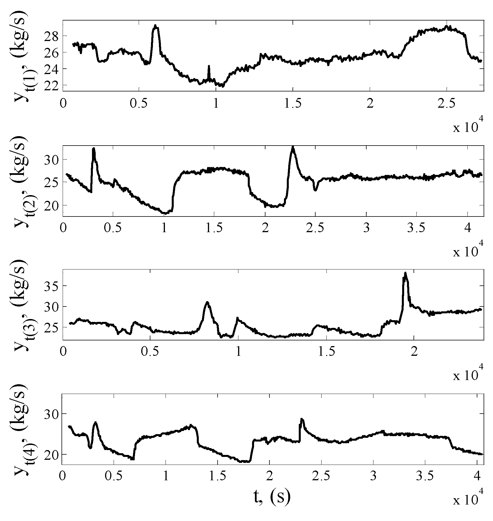
Based on the model developed, the flow rates of the feed solids were determined by stimulating the model with the residuals determined for models with the parameters given in Table 3, and the results are presented in Figure 10.

4.3. Results of Predicting the Flow Rate of Coal Flotation Feed Solids as a Stochastic Process

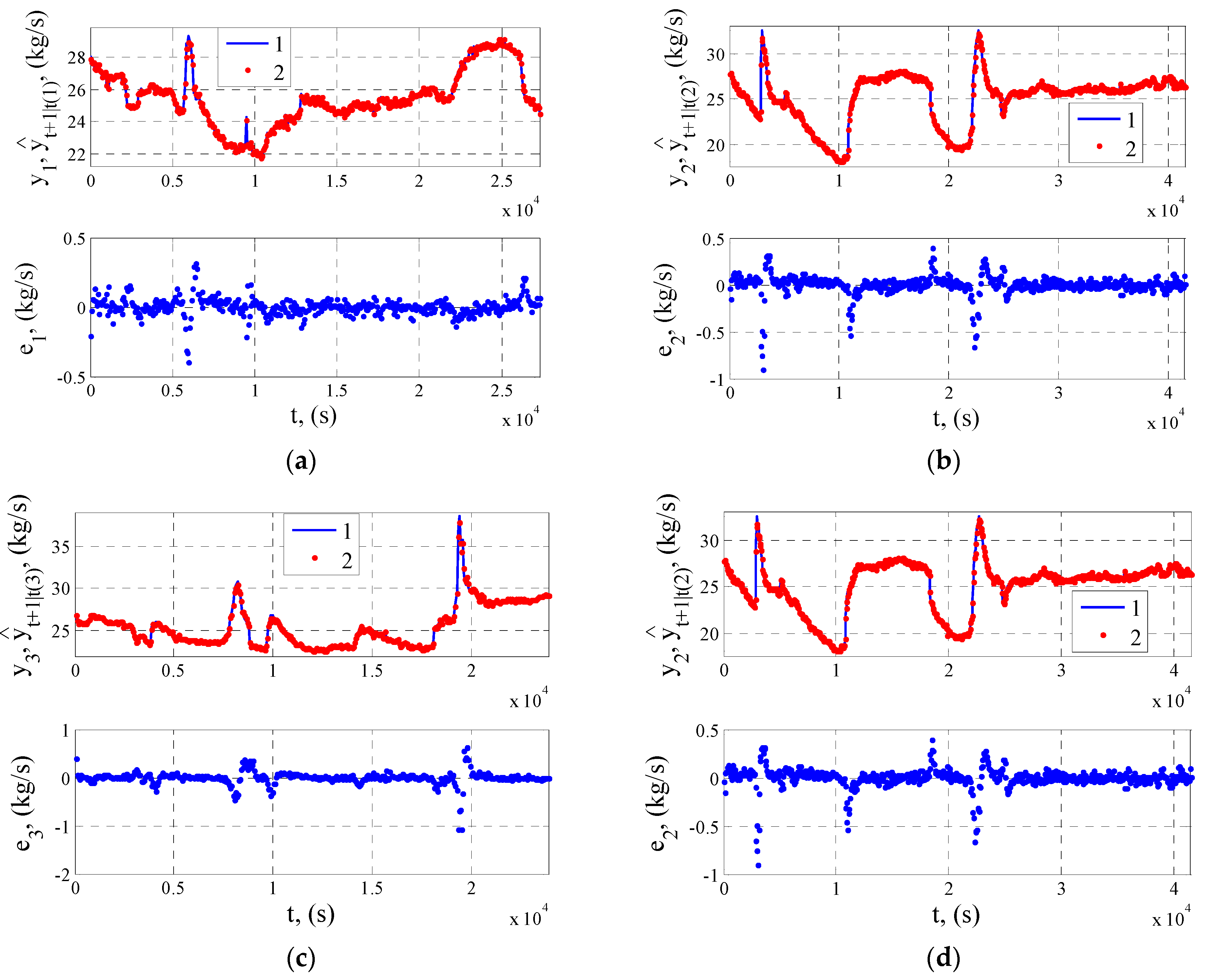
Using Equation (18), it is possible to prepare the predictor equation for the flow rate of the coal flotation feed solids of the industrial process under consideration:

$${\widehat{y}}_{t+1|t}=1.0682+0.2931y_{t-1}-0.3807y_{t-2}-0.1588e_t-0.2301e_{t-1}+0.1037e_{t-2}$$

(22)

Equation (18) was used to determine one-step forecasts for the flow of feedstock solids ${\widehat{y}}_{t+1|t\left(1\right)}, {\widehat{y}}_{t+1|t\left(2\right)}, {\widehat{y}}_{t+1|t\left(3\right)}, {\widehat{y}}_{t+1|t\left(4\right) }$ regarding the recorded courses y₁, y₂, y₃, y₄. The course of the solids in the feed flow prediction determined on the basis of Equation (22) and the prediction errors, for the actual courses as in Figure 3, is shown in Figure 11.

The calculated extreme values of the prediction error obtained for the four data series are presented in

Table 5. Extreme values of the prediction error obtained on the basis of forecasts for four data series.

et (kg/s)
Value	Series 1	Series 2	Series 3	Series 4
min	–0.40	–0.90	–1.08	–1.02
max	0.31	0.40	0.61	2.70

.

5. Discussion

The calculations carried out for the first series of data y₁ and the quantitative evaluation of the adopted criteria indicate that an ARMA model of the fourth order, determined on the basis of a sequence of residuals described by a model of the fifth order, should be used to describe the course of the flow of solids in the feed (Figure 6a). However, the analysis of criteria (7) and (13) for the models determined for the remaining three series of data shows that it is correct to assume n = 3 as the order of the ARMA model with parameters estimated based on a sequence of residuals described by a model of order p = 5 (Figure 6b–d). Therefore, the ARMA model of order n = 3 identified based on the first series of measurement data was adopted for further research. The validity of adopting this order is also confirmed by the results of the residuals obtained for this model analysis. These results, shown in Figure 8, allow us to conclude that the obtained residual sequence can be treated as a white noise sequence, i.e., a residual sequence t is not correlated. This statement is confirmed by the course of the determined normalized autocorrelation function presented in Figure 8b.

The simulation courses generated on the basis of the ARMA model (3) with parameters (21) were used to determine the desired model of the flotation feed solids flow rate. The parameters of this model were taken as the average values of the parameters determined on the basis of 10 simulation courses, the values of which are listed in Table 4. Their standard deviations are also given there. Based on these results, it can be concluded that the model parameters estimated for each series of measurement data (Table 3) are within three times the calculated standard deviations. It should be noted that the developed model reproduces well the time courses of the flow of the solid parts of the feed obtained from the industrial experiment. This is clearly shown in the results presented graphically in Figure 10. As can be seen in this figure, the time courses reconstructed using the ARMA model of Equation (21) stimulated by a sequence of residuals determined for models with the parameters given in Table 3, show satisfactory convergence with the empirical data shown in Figure 5.

The developed model of the flotation feed solids flow rate, as a stochastic process described by the ARMA model, enables the generation of any number of waveforms with the stimulation of a sequence of independent random variables with a zero mean value and the calculated variance σ²_ε = 0.0891. This makes it possible to study the response of automatic systems to random changes in the feed flow rate by computer simulation for many sequences. Thanks to this, it is possible to assess the correctness of the adopted structure of the automatic control system and the controller settings on the basis of simulation and to adjust them to the values that allow the best compensation of the influence of changes in the solids flow rate on the enrichment process. It is a practical aspect related to the design of the automatic control system of the flotation process.

The model of disturbance in the flotation process (21) was used, according to Equation (18), to prepare the equation of the coal flotation feed solids flow rate predictor, which enables prediction of this quantity with the time horizon equal to the sampling period. The courses of solids flow rate predictions presented in Figure 11 show significant convergence with the measured quantity. The value of the prediction error does not exceed 2.7 kg/s. Therefore, it is justified to state that the prediction with the prediction horizon equal to one sampling period based on Equation (22) gives satisfactory results.

Currently, in the situation of manual control, the process operator-expert, based on his experience, and the current (displayed on the monitor) measurements of solids concentration in the feed and, to a lesser extent, the flow rate, decides to change the value (increase or decrease) of key control signals. These are the following quantities: reagent flow rate and air flow for slurry level in flotation cell. Currently, the operator can only react to the indications of current measurements and observe the response of the process to such changes. The developed forecast model can be used by the process operator (manual control) who, based on the predicted forecast of the change in the solids flow rate, can make decisions about changes in such quantities as: the amount of reagent dosed or the value of the air flow rate, before this change in the solids flow rate occurs (action in advance), which can provide faster and more effective compensation for adverse changes in the solids flow rate of the feed. Moreover, the forecast model can be used in the automatic control system-predictive control.

6. Conclusions

Disturbances in the form of time variations in the flow of solids for flotation can be represented as a stochastic process and described by ARMA models. This paper presents an algorithm for the estimation of ARMA model parameters by the double least squares method in application to modelling the flow rate of feed solids for flotation. As shown by the obtained results of identification calculations, the time course of the feed solids flow rate can be modelled as a third-order ARMA process with parameters a₁ = −1.0682, a₂ = −0.2931, a₃ = 0.3807, c₁ = −0.1588, c₂ = −0.2301, c₃ = 0.1037, and variance σ²_ε = 0.0891 determined on the basis of a sequence of residuals with the properties of a white noise sequence. The sequence of residuals is described by a model of the fifth order with coefficients b₁ = −0.9157, b₂ = −0.2023, b₃ = 0.0143, b₄ = −0.0020, and b₅ = 0.1168. The determined model parameters for the measured data, measured during four consecutive periods of continuous operation of the flotation facility, show a significant divergence but fall within the range of three calculated standard deviations. This shows that the parameters of the feed solids flow rate model do not change significantly for four consecutive periods of continuous operation of the industrial facility. It is shown that the estimated parameters of the ARMA model can be used to predict the time series of solids flow in the feedstock with a prediction horizon equal to the sampling period.

For the industrial process for which the identification tests were carried out, the developed ARMA model in qualitative terms is universal. Over time, only the values of the ARMA model parameters may change, but the order of the model will remain the same. In such a case, only the operation of determining the parameter values is necessary., and there is no need to determine the order of the model, which significantly shortens the calculation process of the used method.

It is also important to demonstrate that good results in identifying the feed solids flow with the ARMA model are obtained using the two-step least squares method. This may be useful information for researchers who will undertake research in this field, e.g., in relation to the flotation process of nonferrous ores.

References

- Fecko, P.; Pectova, I.; Ovcari, P.; Cablik, V.; Tora, B. Influence of petrographical composition on coal flotability. Fuel 2005, 84, 1901–1904. [Google Scholar] [CrossRef]
- Fečko, P.; Janakova, I.; Raclavska, H.; Tora, B. Application of flotation in the decontamination of sediments from the Cerny prikop stream. Pol. J. Chem. Technol. 2009, 11, 8–11. [Google Scholar] [CrossRef] [Green Version]
- Niu, C.; Xia, W.; Li, Y.; Bu, X.; Wang, Y.; Xie, G. Insight into the low-rank coal flotation using amino acid surfactant as a promoter. Fuel 2022, 307, 121810. [Google Scholar] [CrossRef]
- Honaker, R.Q.; Jain, M.; Parekh, B.K.; Saracoglu, M. Ultrafine coal cleaning using spiral concentrators. Miner. Eng. 2007, 20, 1315–1319. [Google Scholar] [CrossRef]
- Hornsby, D.T.; Watson, S.J.; Clarkson, C.J. Fine Coal Cleaning by Spiral and Water Washing Cyclone. Coal Prep. 1993, 12, 133–161. [Google Scholar] [CrossRef]
- Cierpisz, S.; Joostberens, J. Simulation of Fuzzy Control of Coal Flotation. IFAC Proc. Vol. 2006, 39, 210–214. [Google Scholar] [CrossRef]
- Dey, S. Enhancement in hydrophobicity of low rank coal by surfactants—A critical overview. Fuel Process. Technol. 2012, 94, 151–158. [Google Scholar] [CrossRef]
- Jia, R.; Harris, G.H.; Fuerstenau, D.W. An improved class of universal collectors for the flotation of oxidized and/or low-rank coal. Int. J. Miner. Process. 2000, 58, 99–118. [Google Scholar] [CrossRef]
- Polat, M.; Polat, H.; Chander, S. Physical and chemical interactions in coal flotation. Int. J. Miner. Process. 2003, 72, 199–213. [Google Scholar] [CrossRef] [Green Version]
- Gui, X.; Xing, Y.; Wang, T.; Cao, Y.; Miao, Z.; Xu, M. Intensification mechanism of oxidized coal flotation by using oxygen-containing collector Îą-furanacrylic acid. Powder Technol. 2017, 305, 109–116. [Google Scholar] [CrossRef]
- Eckert, K.; Schach, E.; Gerbeth, G.; Rudolph, M. Carrier Flotation: State of the Art and its Potential for the Separation of Fine and Ultrafine Mineral Particles. Mater. Sci. Forum 2019, 959, 125–133. [Google Scholar] [CrossRef]
- Bournival, G.; Yoshida, M.; Cox, N.; Lambert, N.; Ata, S. Analysis of a coal preparation plant. Part 2. Effect of water quality on flotation performance. Fuel Process. Technol. 2019, 190, 81–92. [Google Scholar] [CrossRef]
- Zhang, Q.; Niu, C.; Bu, X.; Bilal, M.; Ni, C.; Peng, Y. Enhancement of Flotation Performance of Oxidized Coal by the Mixture of Laurylamine Dipropylene Diamine and Kerosene. Minerals 2021, 11, 1271. [Google Scholar] [CrossRef]
- Zhang, R.; Xia, Y.; Guo, F.; Sun, W.; Cheng, H.; Xing, Y.; Gui, X. Effect of microemulsion on low-rank coal flotation by mixing DTAB and diesel oil. Fuel 2020, 260, 116321. [Google Scholar] [CrossRef]
- Shi, C.; Cheng, G.; Wang, S. Optimization of Coal Washery Tailings by Flotation Process. Energies 2019, 12, 3956. [Google Scholar] [CrossRef] [Green Version]
- Shen, L.; Min, F.; Liu, L.; Xue, C.; Zhu, J. Improving Coal Flotation by Gaseous Collector Pretreatment Method and its Potential Application in Preparing Coal Water Slurry. Processes 2019, 7, 500. [Google Scholar] [CrossRef] [Green Version]
- Ahmed, H.A.M.; Drzymala, J. Upgrading difficult-to-float coal using microemulsion. Min. Met. Explor. 2012, 29, 88–96. [Google Scholar] [CrossRef]
- Chen, Y.; Xu, G.; Huang, J.; Eksteen, J.; Liu, X.; Zhao, Z. Characterization of coal particles wettability in surfactant solution by using four laboratory static tests. Colloids Surf. A Physicochem. Eng. Asp. 2019, 567, 304–312. [Google Scholar] [CrossRef]
- Bu, X.; Xie, G.; Peng, Y.; Ge, L.; Ni, C. Kinetics of flotation. Order of process, rate constant distribution and ultimate recovery. Physicochem. Probl. Miner. Process. 2017, 53, 342–365. [Google Scholar]
- Bu, X.; Xie, G.; Chen, Y.; Ni, C. The Order of Kinetic Models in Coal Fines Flotation. Int. J. Coal Prep. Util. 2017, 37, 113–123. [Google Scholar] [CrossRef]
- Kalinowski, K.; Kaula, R. Verification of flotation kinetics model for triangular distribution of density function of flotability of coal particles / weryfikacja modelu kinetyki flotacji dla trójkątnego rozkładu funkcji gęstości flotowalności ziaren węgla. Arch. Min. Sci. 2013, 58, 1279–1287. [Google Scholar] [CrossRef] [Green Version]
- Sokolovic, J.; Miskovic, S. The effect of particle size on coal flotation kinetics: A review. Physicochem. Probl. Miner. Process. 2018, 54, 1172–1190. [Google Scholar]
- Li, Y.; Zhao, W.; Gui, X.; Zhang, X. Flotation kinetics and separation selectivity of coal size fractions. Physicochem. Probl. Miner. Process 2013, 49, 387–395. [Google Scholar] [CrossRef]
- Brozek, M.; Mlynarczykowska, A.; Turno, A. The relationships between deterministic and stochastic models of flotation. Arch. Min. Sci. 2003, 48, 299–314. [Google Scholar]
- Brozek, M.; Mlynarczykowska, A. Application Of The Stochastic Model For Analysis Of Flotation Kinetics With Coal As An Example. Physicochem. Probl. Miner. Process. 2006, 40, 31–44. [Google Scholar]
- Brozek, M.; Mlynarczykowska, A. Analysis of kinetics models of batch flotation. Physicochem. Probl. Miner. Process. 2007, 41, 51–65. [Google Scholar]
- Clarkson, C.; Hornsby, D.; Walker, D. Automatic Flotation Control using On-Stream Ash Analysis. Coal Prep. 1993, 12, 41–64. [Google Scholar] [CrossRef]
- Laurila, M.J. The Use of On-Line Coal Ash Monitoring Systems in Local Control Applications. Coal Prep. 1994, 14, 81–91. [Google Scholar] [CrossRef]
- Shahbazi, B.; Chelgani, S.C. Modeling of fine coal flotation separation based on particle characteristics and hydrodynamic conditions. Int. J. Coal Sci. Technol. 2016, 3, 429–439. [Google Scholar] [CrossRef] [Green Version]
- Woodbum, E.T.; Wallin, P.J. Decoupled kinetic model for simulation of flotation networks. Trans. Inst. Min. Metall. Sect. C Miner. Process. Extr. Metall. 1984, 93, C153–C161. [Google Scholar]
- Yoon, R.H.; Kelley, K.; Do, H.; Sherrell, I.; Noble, A.; Kelles, S.; Soni, G. Development of a flotation simulator based on a first principles model. In Proceedings of the 26th International Mineral Processing Congress (IMPC 2012), New Delhi, India, 24–28 September 2012; Volume 980, pp. 1–14. [Google Scholar]
- Soni, G. Development and Validation of a Simulator Based on a First-Principle Flotation Model. Master’s Thesis, The Virginia Polytechnic Institute and State University, Blacksburg, VA, USA, 2013; pp. 1–58. [Google Scholar]
- Trybalski, K.; Ciepły, J. ARMA type model for copper ore flotation. Dev. Miner. Process. 2000, 13, C3-72. [Google Scholar] [CrossRef]
- Farnum, N.R.; Stanton, W. Quantitative Forecasting Methods; PWS-Kent Publishing Company: Boston, MA, USA, 1989. [Google Scholar]
- Sen, P.; Roy, M.; Pal, P. Application of ARIMA for forecasting energy consumption and GHG emission: A case study of an Indian pig iron manufacturing organization. Energy 2016, 116, 1031–1038. [Google Scholar] [CrossRef]
- Ediger, V.; Akar, S.; Uğurlu, B. Forecasting production of fossil fuel sources in Turkey using a comparative regression and ARIMA model. Energy Policy 2006, 34, 3836–3846. [Google Scholar] [CrossRef]
- Tasdemir, A. Analysis of chromite processing plant data by first order autoregressive model. Physicochem. Probl. Miner. Process. 2013, 49, 157–174. [Google Scholar]
- Liu, W.Q.; Han, N.; Yan, M.; Tao, G.L. Self-Tuning Fusion Kalman Filter for ARMA Signals. In Applied Mechanics and Materials; Trans Tech Publications, Ltd.: Freienbach, Switzerland, 2012; Volume 229, pp. 1768–1771. [Google Scholar]
- Mayne, D.; Firoozan, F. Linear identification of ARMA processes. Automatica 1982, 18, 461–466. [Google Scholar] [CrossRef]
- Broersen, P.M.; de Waele, S. Automatic Identification of Time-Series Models From Long Autoregressive Models. IEEE Trans. Instrum. Meas. 2005, 54, 1862–1868. [Google Scholar] [CrossRef]
- Ganguli, R.; Tingling, J.C. Algorithms to Control Coal Segregation Under Non–Stationary Conditions. Part II: Time Series Based Methods. Int. J. Miner. Process. 2001, 61, 261–271. [Google Scholar] [CrossRef]
- Durbin, J. The Fitting of Time-Series Models. Rev. l’Institut Int. Stat. Rev. Int. Stat. Inst. 1960, 28, 233. [Google Scholar] [CrossRef]
- Akaike, H. Fitting autoregressive models for prediction. Ann. Inst. Stat. Math. 1969, 21, 243–247. [Google Scholar] [CrossRef]
- Cierpisz, S.; Joostberens, J. Monitoring of coal jig operation using a radiometric meter with a variable time of measurement. IOP Conf. Ser. Mater. Sci. Eng. 2018, 427, 012020. [Google Scholar] [CrossRef] [Green Version]
- Astafieva, I.M.; Gerasimov, D.N.; Makseev, R.E. Density measurement by radiometric method with gamma irradiation from sources of low activity. J. Phys. Conf. Ser. 2017, 891, 012322. [Google Scholar] [CrossRef]
Figure 1.
Coal flotation process as a control object.
Figure 2.
Automatic control of the coal flotation process with a constant reagent dose.
Figure 3.
Prediction of the stochastic process.
Figure 4.
Industrial facility of the coal flotation process: C1, C2—concentrates, O1, O2—flotation waste.
Figure 5.
Time courses of the feed solids flow rate directed to the flotation tank determined on the basis of the solids concentration courses and the feed flow rate recorded at the industrial facility.
Figure 6.
The dependence of criterion (13) on the order n of the ARMA model describing the flow rate of flotation feed solids, determined for a series of measurement data: (a) y1, (b) y2, (c) y3, (d) y4 based on the residuals described by the model of order p = 5.
Figure 7.
Positions of zeros and poles of the ARMA model with parameters (20).
Figure 8.
Evaluation of the ARMA model residuals with parameters (20): (a) course of the residuals, (b) standardised autocorrelation function.
Figure 9.
Examples of simulated feed solids flow rates: (a) series 1, (b) series 4, (c) series 8, (d) series 10.
Figure 10.
Time courses of the feed solids flow rate determined by means of the third-order ARMA model with Equation (21).
Figure 11.
Prediction error and one-step forecast of the flotation feed solids flow rate against measured data; (a) series 1, (b) series 2, (c) series 3, (d) series 4; 1—measured data, 2—forecast.