Numerical Demonstration of Unsupervised-Learning-Based Noise Reduction in Two-Dimensional Rayleigh Imaging

Abstract

The conventional denoising method in Rayleigh imaging in a general sense requires an additional hardware investment and the use of the underlying physics. This work demonstrates an alternative image denoising reconstruction model based on unsupervised learning that aims to remove Mie scattering and shot noise interference from two-dimensional (2D) Rayleigh images. The model has two generators and two discriminators whose parameters can be trained with either feature-paired or feature-unpaired data independently. The proposed network was extensively evaluated with a qualitative examination and quantitative metrics, such as PSNR, ER, and SSIM. The results demonstrate that the feature-paired training network exhibits a better performance compared with several other networks reported in the literature. Moreover, when the flame features are not paired, the feature-unpaired training network still yields a good agreement with ground truth data. Specific indicators of the quantitative evaluation show a promising denoising ability with a peak signal-to-noise ratio of ~37 dB, an overall reconstruction error of ~1%, and a structure similarity index of ~0.985. Additionally, the pre-trained unsupervised model based on unpaired training can be generalized to denoise Rayleigh images with extra noise or a different Reynolds number without updating the model parameters.

1. Introduction

Rayleigh scattering has been demonstrated to be a useful tool for diagnosing gas-phase flow properties not only in non-reacting flows but also in reacting flows. While it is not a species-selective technique, several key parameters can be deduced from the Rayleigh signal with certain assumptions. The flow properties that can be measured include flow temperature [1,2], mixture fraction [3], fuel concentration [4], velocity [5], and scalar dissipation [6,7]. Planar Rayleigh imaging is very appealing because it can visualize two-dimensional (2D) flow/flame details with a small hardware investment and a relatively strong signal level [1]. As an elastic process, the wavelength of Rayleigh scattering is very close to that of the probe laser, making it vulnerable to all kinds of laser-induced illuminations. In particular, when the diameters of dust, liquid droplet, or other particles in the flowfield are comparable with the wavelength of the probe laser, strong Mie scattering noise might severely disturb the Rayleigh images and deteriorate the accuracy of the Rayleigh measurements.

Considerable efforts have been made to reduce the noise in the Rayleigh measurements over the past few decades. The most straightforward method takes advantage of the signal level difference since Mie scattering is typically orders of magnitude stronger than Rayleigh scattering. It has been demonstrated that Mie scattering noise can be identified and eliminated using the amplitude threshold and fast rise filtering in pointwise measurements [8]. As another approach, varying polarization characteristics of different light sources have also been utilized to differentiate the Rayleigh signal from intensive laser glare or background radiation in experiments on a turbulent combustor with poor optical access [9]. Futhermore, with the aid of an ultrathin molecular notch filter, the filtered Rayleigh scattering (FRS) technique utilizes varying spectral widths to differentiate the Rayleigh signals from the Mie scattering noise [1,2,10]. Structured laser illumination planar imaging (SLIPI) uses an intensity-modulated laser sheet to measure the 2D temperature field while substantially mitigating the interference of spurious light [11,12]. All these methods have been extensively studied and applied in the past, and their capabilities and limitations are relatively well understood. A common limitation to all these approaches is that they involve an additional hardware investment and an in-depth understanding of the underlying physics of Rayleigh scattering. On the other hand, a contaminated Rayleigh image can be treated as a clear Rayleigh image superimposed with noise, including Mie scattering noise, stray light, and shot noise. Therefore, noise reduction in Rayleigh imaging is a problem of image processing. This work focuses on image processing techniques, in other words, on removing high-value Mie scattering noise while maintaining the Rayleigh signal in its original form as much as possible.

Traditional image denoising methods use predefined filters, such as median filters or Gaussian filters, to smooth out the high-value pixels and random white noise [13,14]. Some algorithms transform the image into the frequency domain and directly drop out high-frequency components [14,15]. The denoised image is realized by transforming the image back into the pixel spatial domain. When applying such a denoising process, high-frequency information or detailed textures in the images will be depleted, leading to an inaccurate or unnatural reconstruction result. With the advancement of high-performance GPU devices and deep learning techniques, recent research has demonstrated the feasibility of denoising images with deep neural networks. Deep-learning-based image processing has been widely demonstrated in many fields, such as super resolution [16], noise reduction [17], and style transformation [18]. The authors have proposed a three-dimensional (3D) super-resolution generative adversarial network (3D-SRGAN) and improved the 3D resolution when applying it to a turbulent jet flame [19]. Cai et al. demonstrated a generative adversarial network (DNGAN) for noise reduction in 2D Rayleigh images based on supervised learning [20] in which the noisy input image and the clear ground-truth Rayleigh image are paired in terms of flame textures. The requirement of feature-paired data limits the potential of such a technique in real experiments, where it is difficult to record the clear and noisy Rayleigh images simultaneously. To overcome the limitation of feature-paired data, an unsupervised learning strategy may be employed. Kim et al. proposed an unsupervised 2D super-resolution model for reconstructing very fine turbulent flow structures through a cycle-consistent generative adversarial network (CycleGAN), which overcomes the limitation of the paired dataset and demonstrates the feasibility of unsupervised learning of turbulent features [18,21].

With the above-described background, the goal of this work is to demonstrate the potential of using unsupervised learning to eliminate the Mie scattering and shot noise in Rayleigh images. The novelty of this work is the integration of the CycleGAN architecture into the synthesized Rayleigh image to develop a noise reduction algorithm without supervision. This algorithm does not require the noisy and noise-free images to be feature-paired as in our previous publication [20]. Therefore, this paper is a further extension of our previous work. Section 2 introduces the data generation and model architecture in detail. Section 3 presents the results and a discussion. Section 4 concludes this paper.

2. Numerical Analysis and Methodology

In this section, the architecture of the denoising network, including the data generation process, network training and testing, and convergence characteristics, is explained in detail.

2.1. Data Generation

In this work, the training data were synthesized from numerically simulated Rayleigh images and experimentally acquired Mie scattering images. Large eddy simulation (LES) was used to generate turbulent flame data (Sandia flame B and C) [22]. The process of validating the jet flame simulation has been described in our previous work [20,22], so only a brief description is provided here. This flame has been extensively studied using both computational simulation and experiments and exhibits strong turbulence–chemistry interaction [23,24]. A partially premixed CH₄/air flow issued from a central nozzle (7.2 mm in diameter) that was surrounded by a pilot flame and an air co-flow. The governing equations were reactive Navier–Stokes equations that take into account a 16-component CH₄/air skeletal mechanism [25], and they were solved using the finite volume method. The Samgorinsky–Lily sub-grid model was used in the simulation to close the governing equations. The eddy dissipation concept (EDC) was used to deal with the turbulence–chemistry interaction, assuming that the molecular mixing and subsequent combustion occurred at fine scales. The boundary conditions for the main jet, pilot flame, and co-flow were set according to previous experiments [23]. The increment time step was set to 1 × 10⁻⁵ s, which is small enough to capture the dynamic characteristics of the flame. The main jet Reynolds number was 8200 for flame B and 1.3 × 10⁴ for flame C.

After completing the above-described simulation, the central slices of the 3D flame were extracted. Through a ray-tracing imaging computation as demonstrated in our previous work [20,26], we obtained clear 2D Rayleigh images. Figure 1a–c illustrate sample views of the 3D temperature isosurface, the 2D temperature slice, and the corresponding 2D Rayleigh images of the turbulent jet flame, respectively. The slice view of the flowfield in Figure 1b includes both the high-temperature central reacting region and the low-temperature surrounding region. The Rayleigh image presented in Figure 1c does not contain any noise, and the noise generation process is described in the following section. It is noted that the typical magnitude of the Rayleigh signal is around 600 for the cold air region, while the magnitude of the signal in the high-temperature region of the flame is much smaller due to the lower local number density. Clear Rayleigh images as shown in Figure 1c were adopted as ground truth targets in neural network training and testing.

Concerning the noisy Rayleigh image, the Mie scattering and shot noise were taken into consideration as demonstrated in Figure 2. Figure 2a was taken to be the same as Figure 1c for comparison purposes. For the Mie scattering interference, we manipulated an experimentally acquired noisy Mie scattering image to generate training data. A frequency-doubled solid-state Nd:Yag laser operating at a 10 Hz repetition rate was used to illuminate a plane of the flow region. The pulse duration was around 9 ns, and the output beam was reshaped into a thin sheet with a vertical height of 50 mm. The pulse energy used in the experiment was 1.2 J in order to ensure that almost every small particle in the flow was illuminated. Due to the presence of dust particles in the air, the Mie scattering signal could be observed in the recorded images. The pixel resolution of the original Mie scattering image was 1024 × 1024, and it was down-sampled to 512 × 512. Several sub-regions with a size of 256 × 256 were then randomly cropped to generate corresponding noise images that were the same size as the clear Rayleigh images. A sample Mie scattering image, I_Mie, is presented in Figure 2b. Once both the clear Rayleigh image and the Mie scattering noise image had been prepared, the two were superimposed to yield a preliminary noisy Rayleigh image, I_WM, as shown in Figure 2c. It is worth noting that the particles were not fully randomly distributed in the jet flame but concentrated in the low-temperature region due to entrainment of air from the atmosphere and destruction during the combustion process. Therefore, a prerequisite regarding the local Rayleigh intensity was set in order to ensure that local Mie scattering interference would be added only when the local Rayleigh intensity threshold was reached.

In addition to Mie scattering noise, shot noise was also considered in this work. It makes this work different from our previous publication [20] and closer to a practical situation since shot noise is a source of unavoidable error during the imaging process. Shot noise is related to the light intensity and obeys a Poisson distribution. The probability function of the Poisson distribution is as follows:

$$P\left(X=k\right)=\frac{{\lambda }^k}{k!}{e}^{-\lambda }$$

(1)

where λ represents the expectation and variance. Figure 2d shows the ultimate noisy Rayleigh image, I_WMS, with both Mie scattering and shot noise. In addition, I_WMS is slightly blurred compared with Figure 2c due to the addition of Poisson noise, although it is not quite evident in Figure 2d. To obtain a more direct sense of the signal patterns, Figure 3 demonstrates the intensity variations along three lines (Z = 40, 100, and 160) as marked in Figure 2d. It is obvious that the relative intensity of the Mie scattering signal is ~6 times higher than that of the Rayleigh signal of the surrounding cold air, and some very strong Mie scattering noise would be saturated. This is in accordance with a realistic situation due to the limited dynamic range of the imaging camera. Moreover, Figure 3 presents obvious signal intensity oscillations in the cold air region, while in the central region the signal variation is not as obvious. According to the shot noise theory, the lower signal intensity might result in more obvious shot noise. The absolute signal magnitude is smaller in the central region, and the oscillation is also much smaller and visually mitigated. Hence, as shown in Figure 3, the oscillation of the Rayleigh signal due to shot noise in the cold region is more significant than in the central region of the flame. Once the clear Rayleigh image shown in Figure 2a and the noisy counterpart shown in Figure 2d have been prepared, they can be used to train the parameters of the neural network in either a supervised or an unsupervised manner. We then conducted a series of simulations and repeated the aforementioned operations, obtaining a training dataset containing 400 time intervals of flame C and a test dataset containing 20 time intervals of flames B and C.

2.2. Denoising Model Architecture

In this work, we propose an unsupervised learning algorithm based on the CycleGAN architecture [18]. The CycleGAN architecture consists of two generators (G and F) and two discriminators (D_X and D_Y), as shown in Figure 4. The generators G and F inter-transform the noisy and noise-free images, while the discriminators D_X and D_Y distinguish the model-generated noisy and noise-free images from the real counterparts. Compared with the DNGAN network reported previously by the authors [20], the network in this work can be trained with either paired or unpaired data, which means that the input topography of the clear and noisy Rayleigh images can be different. This strategy removes the necessity of obtaining clear and noisy Rayleigh images simultaneously and enhances the potential application of a learning-based method in a practical Rayleigh scattering experiment.

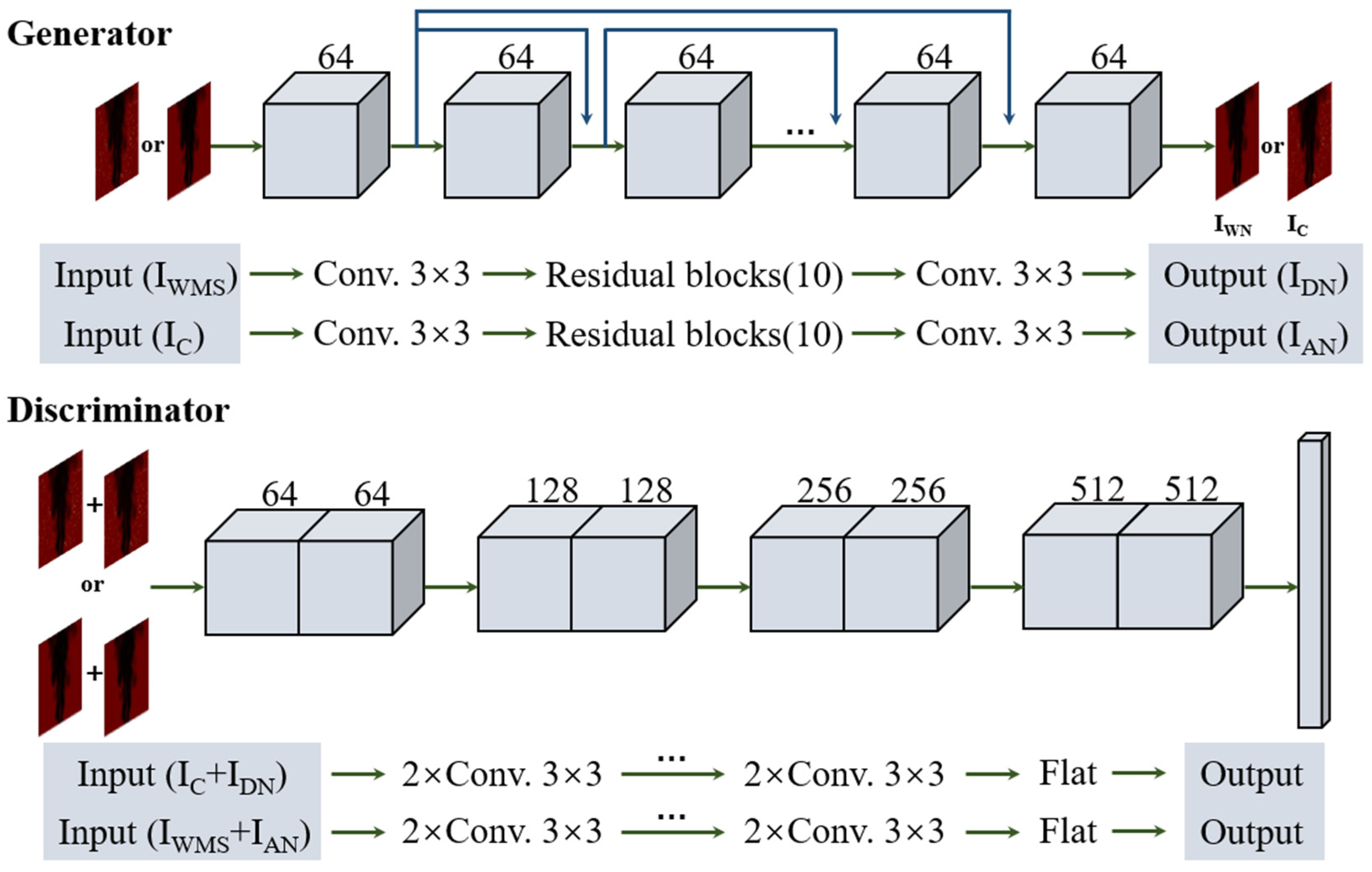
Figure 5 illustrates the architecture of the generators and the discriminators. Note that the architectures of the two discriminators, D_Y and D_X, and the two generators, G and F, are essentially the same. For that reason, only one generator and one discriminator are shown in Figure 5. The structure of the generator (G or F) can be seen on the upper side of Figure 5. The number of output channels and the number of strides were uniformly set to 64 and 1, respectively, for 2D convolution with a kernel size of 3 × 3, which considers a tradeoff between network performance and computational cost. In addition to 2D convolution, other operations, including batch normalization, the leaky ReLU function, residual blocks, and a skip connection, are indicated by the blue arrows in Figure 5. The main effect of the BN layers is to change the data distribution, ensuring that it lies in the sensitive interval of the activation function in order to avoid gradient disappearance [27]. The use of BN layers is also expected to speed up the convergence of the network since the intensity variation from batch to batch is eliminated. In the parameter tuning process, we tried to remove the BN layers, which made it more difficult for the iteration process to converge to a stable state and resulted in poor denoising quality. The activation function is known to be an effective tool for stabilizing the weight parameters during the learning process. We tried both the ReLU and the leaky ReLU functions, and the latter was found to give a slightly better performance, although both functions performed well [28]. A combination of residual blocks and a skip connection can help to avoid gradient dispersion [29] and deepen the network without extra coding. For the network used here, each residual block contained two batch normalizations, two convolutional layers, and one ReLU layer. The number of residual blocks was set to 10, since the denoising ability of a network tends to saturate when the number reaches 10. At the end of each generator, an activation layer was used to output the denoised image, I_DN, or the noisy image, I_AN. The structure of the discriminator (D_X or D_Y) can be seen on the lower side of Figure 5. The number of output channels progressively increased from 64 to 512 from the start to the end. Each pair of convolutional layers was combined into one group operation. The former contained a 2D convolution and a ReLU layer with a stripe of 1, while the latter contained one more batch normalization with a stripe of 2. The result was a long vector of 131,072 elements with characteristics obtained by a sigmoid activation layer.

The loss function measures the difference between the predicted results and the ground truth, although the flame patterns of those two are not necessarily the same in unsupervised learning. The essence of the training process is to minimize the loss function, and thus build a nonlinear mapping between clear and noisy Rayleigh images. The loss function used in this work includes both forward and backward propagation due to the particular architecture of the CycelGAN learning model. In particular, the weighted sum of the mean square error loss, L_MSE, the adversarial loss, L_adv, and the cycle-consistency loss, L_cycle, constitutes the loss function of generators, L_gen,

$$L_{gen}=L_{MSE}+\beta \times L_{adv}+\gamma \times L_{Cycle}$$

(2)

where β and γ are hyper-parameters, which were set to 1 × 10⁻³ and 10, respectively [16,18]. L_MSE is defined through a pixel-by-pixel comparison, as displayed in Equation (3),

$$L_{MSE}=\frac{1}{WH}{\displaystyle \sum }_{pixel}{\left(I_C-I_{DN}\right)}^2+\frac{1}{WH}{\displaystyle \sum }_{pixel}{\left(I_{WMS}-I_{AN}\right)}^2$$

(3)

where W is the width and H is the height of the image, and I_DN and I_AN are the output results of G and F, respectively. The adversarial loss, L_adv, represents the perceptual agreement between the output of the generator and the ground-truth image and prevents the output results from being over-smoothened. The definition of L_adv is presented in Equation (4):

$$L_{adv}=-{\displaystyle \sum }_{pixel}log{D}_X\left(G\left(I_{WMS}\right)\right)-{\displaystyle \sum }_{pixel}log{D}_Y\left(F\left(I_C\right)\right)$$

(4)

where G and D_Y are the generator and discriminator in the forward propagation, respectively, and F and D_X are the generator and discriminator in the back propagation, respectively. The third term in Equation (2), L_cycle, is the core of the generator loss function. In the definition of L_cycle in Equation (5), G(F(I_C)) represents the result of adding noise and then denoising the image, while F(G(I_WMS)) represents the result of denoising the image and then adding noise. Hence, L_cycle essentially refers to the error of transforming an input image to the source domain after passing it through the two generators. Ideally, no difference should be found on a frame after passing it though the two generators.

$$L_{Cycle}=\frac{1}{WH}{\displaystyle \sum }_{pixel}\left(I_C-G(F\left(I_C\right)\right)+\frac{1}{WH}{\displaystyle \sum }_{pixel}\left(I_{WMS}-F(G\left(I_{WMS}\right)\right)$$

(5)

The loss function of the discriminators is defined by the sum of two feature distributions for clear and noisy images, as shown in Equation (6):

$$L_{dis}=\left(D_Y\left(I_{DN}\right)-D_F\left(I_C\right)\right)+\left(D_X\left(I_{WMS}\right)-D_X\left(I_{AN}\right)\right)$$

(6)

2.3. Model Training and Testing

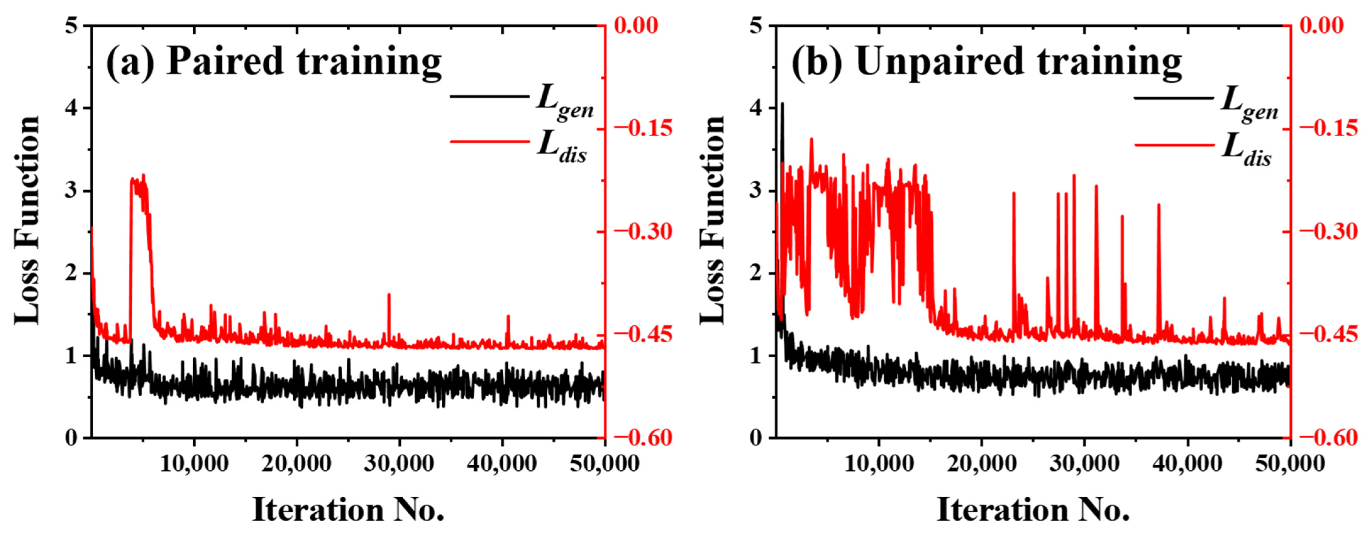
Once the training data have been prepared and the learning model has been constructed, the network can be trained and tested. The proposed model was realized based on the Tensorflow framework and trained with two Nvidia RTX-2080TI GPUs. The model parameters were determined using the adaptive moment estimation (Adam) algorithm [30]. When the model had 10 residual blocks and the learning rate was set to 0.0002, four hours of training were needed to achieve a convergent solution with 50,000 iterations. By alternately training the generators and the discriminators, the denoising result of the generator was good enough that the discriminator confused the denoising result with the corresponding ground truth image. In this work, the network was trained twice (once with feature-paired data and once with feature-unpaired data). In the feature-paired data, the flame features and patterns were the same between noisy Rayleigh images and clear ground-truth images. The only difference is that the Rayleigh images are noisy and the ground-truth images are not. Correspondingly, in the feature-unpaired data, the flame patterns in noisy and clear images can be adopted from different time instants. In this case, simultaneous acquisition of the clear and noisy images is not necessary. Figure 6 presents evolutions of the loss functions during the training process with feature-paired data and feature-unpaired data, respectively. For a pre-trained network, the time required to generate a denoising result is approximately 10 milliseconds. The loss function values tend to converge similarly. Once the network converges to a steady state, an indistinguishable denoising solution has been generated such that the output of the generator G can deceive the discriminator D_Y effectively.

3. Results and Discussion

This section presents the performance of the proposed network both qualitatively and quantitatively. First, the denoising model trained by the feature-paired dataset was used for a preliminary validation and compared with several other denoising models from the literature, including DNGAN [20], DNCNN [31], and RESTNET [32]. It should be noted that the other three other networks used the same forward inference network as G in CycleGAN in order to guarantee a comparable baseline. The discriminator of DNGAN was similar to D_Y of CycleGAN. The same hyperparameters were used for these networks, except that the learning rate of DNGAN, DNCNN, and RESTNET was set uniformly to 0.0001. Moreover, the model trained with the unpaired dataset further extends the application potential to cases where no clear Rayleigh images are available. The remainder of this paper deals with detailed outcomes.

3.1. Network Performance Based on Feature-Paired Training

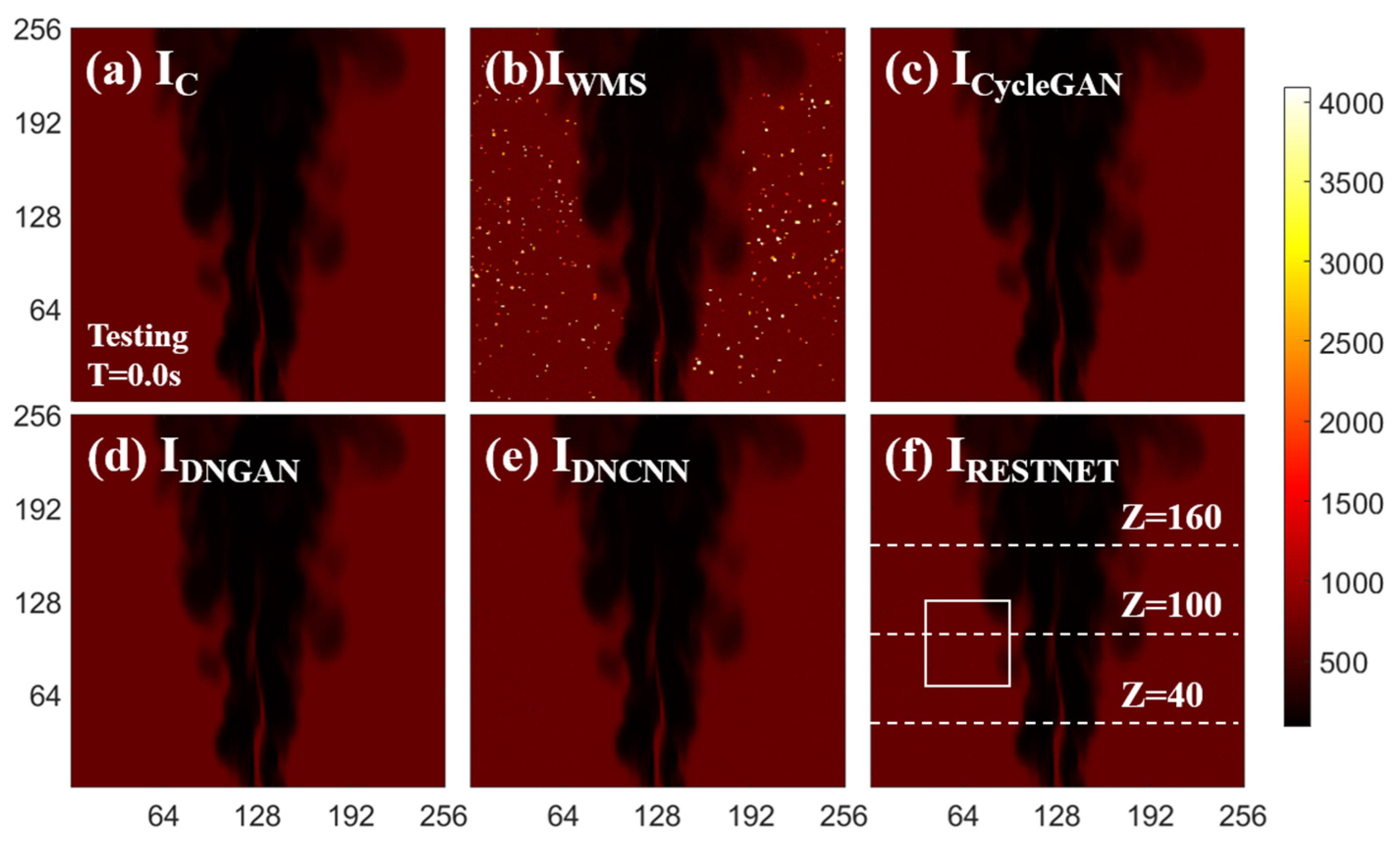
As a preliminary examination, the feature-paired dataset was used to train the proposed network and the three other aforementioned networks, i.e., DNGAN, DNCNN, and RESTNE. These four pre-trained models were tested using 20 noisy Rayleigh images (flame C). Figure 7a,b demonstrate the clear and noisy images with Mie scattering noise and shot noise for comparison purposes. Figure 7c–f show the denoising results obtained by taking advantage of the trained four networks. As can be seen, each model achieves a good level of noise purification and there are no sensible dissimilarities in Figure 7c–f. This is due in part to the limited zoom ratio. To better illustrate the visual difference, the smaller boxed areas shown in Figure 7f were amplified and are presented in Figure 8a–d. There is sensible high-value noise that has not been removed completely in the denoising results of DNCNN and RESTNET, while CycleGAN and DNGAN yield much better denoising results.

Figure 9 presents a comparison of the intensity variation in the denoising results along the three horizontal lines marked by dashed white lines in Figure 7f with Z = 40, 100, and 160, respectively. We can see that the intensity variations of CycleGAN and DNGAN are in very good agreement with the ground truth. This implies that the two algorithms not only effectively suppress the noise caused by Mie scattering and shot noise, but also accurately recover the original Rayleigh signal variation. DNCNN and RESTNET exhibit obvious deviations from the ground truth variation, and the high-value noise points have not been completely eliminated, as already shown in Figure 8c,d. Furthermore, all four networks were able to preserve the intensity variation in the central region, implying a good feature learning capability for shot noise.

To further quantitatively evaluate the denoising performance, three metrics, i.e., the peak signal-to-noise ratio (PSNR) [33], the overall reconstruction error (E_R) [34], and the structural similarity index (SSIM) [35], are shown in Figure 10. The PSNR is widely used to assess the pixel-to-pixel difference between two images by measuring the peak signal to mean signal ratio. The E_R is commonly used to measure the overall correspondence between two images, with a smaller E_R value representing a better match. The SSIM is a standard indicator used to compare the similarity of the structure, contrast, and intensity between two images. A larger SSIM signifies a higher degree of similarity, and the SSIM value would be 1 for two identical images. As can be seen from Figure 10a, the PSNR of the CycleGAN and DNGAN frameworks is consistently greater than 40, which outperforms DNCNN and RESTNET. Figure 10b,c compare the E_R and the SSIM among the networks. It can be seen that CycleGAN and DNGAN maintain an absolute advantage with lower E_R and higher SSIM values. Additionally, DNGAN is slightly better than CycleGAN according to Figure 10.

3.2. Network Performance Based on Feature-Unpaired Training

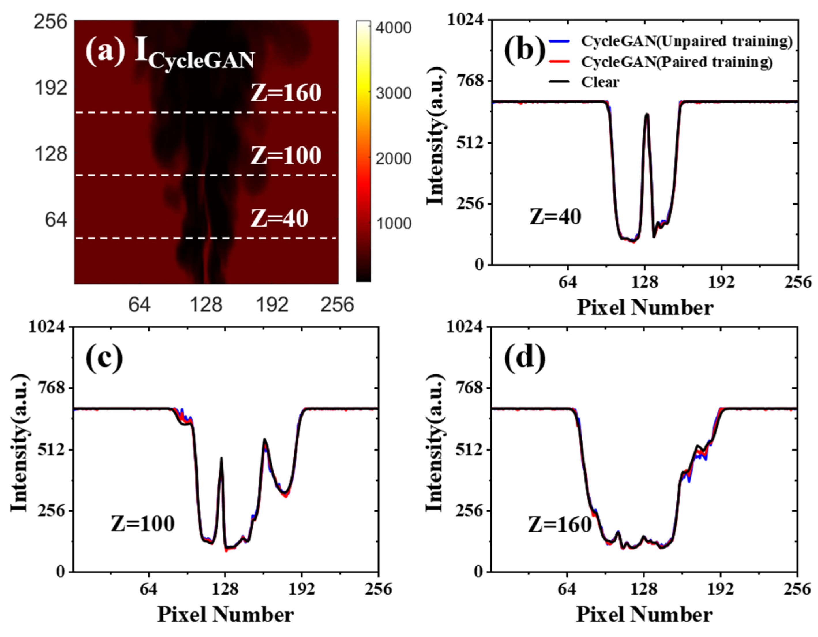
As mentioned above, feature-paired training of the framework yields good denoising results. Notwithstanding, a paired dataset with the same flame patterns is usually not easy to obtain in a practical experiment due to the dynamically varying turbulent flow structure. In this subsection, therefore, the CycleGAN network’s performance is discussed based on feature-unpaired training. In this case, the CycleGAN network was retrained one more time with the unpaired data. The evolutions of the corresponding loss functions are displayed in Figure 6b. To comprehensively evaluate the performance of the network, the retrained model was tested under three test scenarios: (1) noisy Rayleigh images of flame C as already demonstrated on the paired training network; (2) noisy Rayleigh images with noise of varying strengths; and (3) a set of flame data on flame B with a different Reynolds number. Similarly to the evaluation with feature-paired training, Figure 11 presents a qualitative and quantitative comparison for a sample case from CycleGAN that is based on feature-unpaired training. According to a visual examination of Figure 11a, the CycleGAN network is able to remove the high-value Mie scattering noise in the low-temperature region. The denoised Rayleigh image is quite close to the corresponding noise-free image, as shown in Figure 7a, making them indistinguishable to the naked eye. Figure 11b–d further illustrate the variation in the Rayleigh intensity along three horizontal lines with Z = 40, 100, and 160 as depicted in Figure 11a. In Figure 11b–d, the blue lines represent the intensity variation in the denoised result based on feature-unpaired training, while the red and black lines represent the denoised result based on feature-paired training and the ground truth variation corresponding to Figure 7a,c, respectively. On the other hand, the blue line deviates from the variation in the clear image more than the red line, although the deviation is not as apparent. This means that the performance of the neural network depends on both the neural network’s architecture and the training data. It is noted that the three other networks (DNGAN, DNCNN, and RESTNET) are not shown here, since they failed to output an acceptable result when the training data were not feature-paired. Since DNGAN, DNCNN, and RESTNET are supervised-learning-based models, they all require a feature-paired dataset in which the flame patterns of noisy and clear images are the same. When fed feature-unpaired data, the objectives for the models to learn are wrong. No matter how many iterations are performed, they cannot correctly learn the underlying physics of noise addition. However, the CycleGAN model’s objectives are not only to reconstruct a clear image from the noisy version, but also to generate a noisy image from the clear version. From this perspective, CycleGAN is essentially transferring the style of the images, which is a key capability of the unsupervised model.

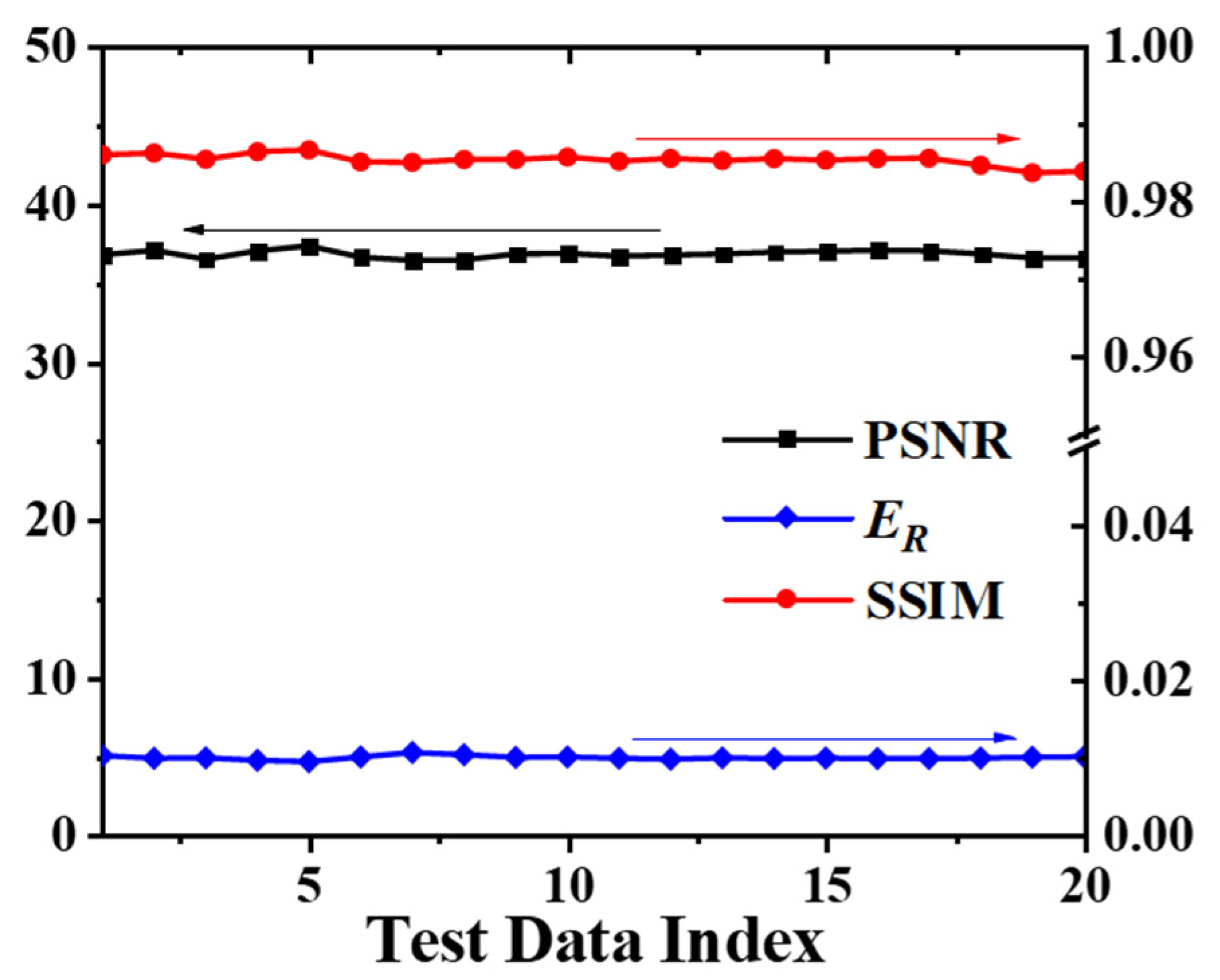
Similarly, the variations in the PSNR, the E_R, and the SSIM of the denoised results were obtained and are shown in Figure 12. In Figure 12, the PSNR corresponds to the left Y-axis, while E_R and the SSIM correspond to the right Y-axis. Each of these three assessment metrics remains on a non-varying level, which means that the performance of the trained network is stable for the test data. Several observations can be made from Figure 12. The mean values of the PSNR, E_R, and SSIM are 37 dB, 1%, and 0.985, respectively. These values are at the same level as those of DNCNN and RSTNET (Figure 10) but are not as outstanding as those of the DNGAN network. However, the visual reconstruction quality of Figure 11 is significantly better than the results of DNCNN and RESTNET (Figure 9). A reasonable explanation is the definition of the loss function and the network architecture. As mentioned above, the generator loss in the forward propagation model consists of the content loss, the adversarial loss, and the cycle-consistency loss, allowing the denoising model to learn potential feature textures more comprehensively. The DNCNN and RESTNET loss functions contain only L2 regularization, which is not sufficient to retain the natural pattern of the turbulent flame. Moreover, compared with DNCNN and RESTNET, the adversarial training of the GAN model updates the model parameters (G and F) according to the back propagation of the discriminators (D_X and D_Y). The difference in performance implies that the PSNR alone cannot guarantee the best solution and more assessment parameters should be used to comprehensively evaluate a neural network model. Nevertheless, Figure 11 and Figure 12 illustrate that the proposed unsupervised model can yield high denoising quality in cases where feature-paired clear and noisy images are not accessible.

In addition to the basic demonstration of the unsupervised model, the noise immunity of our network due to the randomness of the Mie scattering intensity in the experiment was also investigated. In the Rayleigh imaging process, the intensity of Mie scattering noise may vary due to the particle density, laser irradiance, observation angle, and so on. Therefore, it is necessary to take into account the denoising performance of the proposed model when it is subjected to different levels of noise. Without updating the model parameters based on feature-unpaired training, the denoising performance with varying levels of noise was examined, and the results are shown in Figure 13. Noise of different magnitudes was added to the test data on flame C in accordance with Equation (7), which is defined on a pixel-to-pixel basis:

$$I_{WMS}=Mode{l}_{Poisson}\left(I_C+I_{Mie}\left(1+\sigma \right)\right)$$

(7)

where σ represents the number of times extra Mie scattering noise was added, and Model_Poisson represents the Poisson modeling process. The newly generated noise in Equation (7) is not simply proportional to the previously added noise. Note that when σ is zero, I_WMS represents the above-described results from Figure 2, Figure 3, Figure 4, Figure 5, Figure 6, Figure 7, Figure 8, Figure 9, Figure 10, Figure 11 and Figure 12. Figure 13 shows the denoising results of the network with σ = 25%, 50%, and 100%, as evaluated by the three metrics of the PSNR, the E_R, and the SSIM. As can be seen from Figure 13, the three parameters almost remain unchanged with σ = 25% and 50%, and the variations in the two cases are almost identical. On the condition that σ increases to 100%, the E_R value exhibits a small deviation, while the corresponding PSNR and SSIM values have not changed significantly compared to σ = 25% and 50%. Noisy Rayleigh images with even higher intensities were not examined further, considering the limited dynamic range of the data acquisition devices used in practical experiments. According to Figure 13, when subjected to more intense Mie scattering noise, the proposed model demonstrates satisfying reconstruction quality and good noise immunity. It should be noted that the model parameters of the network were not updated when tested with more intense noise. Improved noise immunity could therefore be expected if enhanced noisy data are used in the network training process.

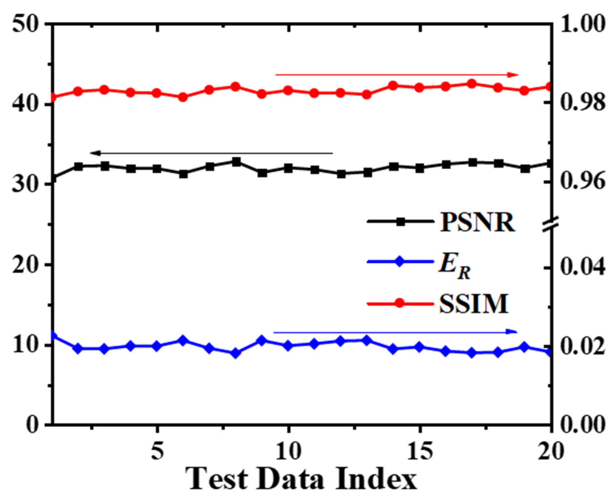
For the purpose of further evaluating the generalization ability of the proposed unsupervised model, another set of test data on flame B was used to evaluate the denoising performance. Correspondingly, the model parameters were not updated during testing. The main jet Reynolds number of turbulent flame B was 8200, which is smaller than that of flame C. We selected 20 snapshots at different time instants and added Mie scattering and shot noise accordingly. By feeding the noisy images into the trained unsupervised network, the variations in the PSNR, the E_R, and the SSIM were calculated. As illustrated in Figure 14, the unsupervised model exhibits a satisfying denoising ability when tested on flames with different structures. The mean values of the PSNR, the E_R, and the SSIM are 33.5 dB, 2%, and 0.983, respectively, which proves that our unsupervised model has a good generalization ability for varying Reynolds numbers.

4. Conclusions

In this work, an unsupervised denoising and image reconstruction model for 2D Rayleigh imaging based on the CycleGAN architecture was developed and demonstrated. Both intense Mie scattering noise and shot noise were considered in this work. When trained with both feature-paired and feature-unpaired datasets, the model was able to overcome the limitation of paired data and showed potential for application in practical experiments. When trained with feature-paired data, the proposed unsupervised denoising model performed as well as the state-of-the-art supervised learning network. When trained with feature-unpaired data, the model’s performance degraded slightly, but it was still able to provide visually indiscernible results. Further examinations with varying noise intensities and flames with different Reynolds numbers showed that the proposed network has a promising generalization capability. In future work, we will focus on using experimental means to obtain all experimental data and promoting our model with more practical perspectives in realistic Rayleigh imaging measurement scenarios.

References

1. Pu, J.; Sutton, J.A. Quantitative 2D thermometry in turbulent sooting non-premixed flamesusing filtered Rayleigh scattering. Appl. Opt. 2021, 60, 5742–5751. [Google Scholar] [CrossRef] [PubMed]
2. McManus, T.A.S.; Jeffrey, A. Quantitative planar temperature imaging in turbulent non-premixed flames using filtered Rayleigh scattering. Appl. Opt. 2019, 58, 2936–2947. [Google Scholar] [CrossRef]
3. Patton, R.A.; Gabet, K.N.; Jiang, N.; Lempert, W.R.; Sutton, J.A. Multi-kHz mixture fraction imaging in turbulent jets using planar Rayleigh scattering. Appl. Phys. B 2012, 106, 457–471. [Google Scholar] [CrossRef]
4. Espey, C.; Dec, J.E.; Litzinger, T.A.; Santavicca, D.A. Planar laser rayleigh scattering for quantitative vapor-fuel imaging in a diesel jet. Combust. Flame 1997, 109, 65–86. [Google Scholar] [CrossRef]
5. Gustavsson, J.P.R.; Segal, C. Filtered Rayleigh scattering velocimetry—Accuracy investigation in a M = 2.2 axisymmetric jet. Exp. Fluids 2005, 38, 11–20. [Google Scholar] [CrossRef]
6. Frank, J.H.; Kaiser, S.A. High-resolution imaging of dissipative structures in a turbulent jet flame with laser Rayleigh scattering. Exp. Fluids 2008, 44, 221–233. [Google Scholar] [CrossRef]
7. Buch, K.A.; Dahm, W.J.A. Experimental study of the fine-scale structure of conserved scalar mixing in turbulent shear flows. Part 2. Sc ≈ 1. J. Fluid Mech. 1998, 364, 1–29. [Google Scholar] [CrossRef]
8. Green, H.G. Developments in signal analysis for laser Rayleigh scattering. J. Phys. E Sci. Instrum. 1987, 20, 670–676. [Google Scholar] [CrossRef]
9. Barat, R.B.; Longwell, J.P.; Sarofim, A.F.; Smith, S.P.; Bar-Ziv, E. Laser Rayleigh scattering for flame thermometry in a toroidal jet stirred combustor. Appl. Opt. 1991, 30, 3003–3010. [Google Scholar] [CrossRef] [PubMed]
10. Miles, R.B.; Lempert, W.R.; Forkey, J. Instantaneous velocity fields and background suppression by filtered Rayleigh scattering. In Proceedings of the 29th AIAA Aerospace Sciences Meeting, Reno, NV, USA, 1 January 1991. [Google Scholar]
11. Kempema, N.; Long, M. Quantitative Rayleigh thermometry for high background scattering applications with structured laser illumination planar imaging. Appl. Opt. 2014, 53, 6688–6697. [Google Scholar] [CrossRef]
12. Kristensson, E.; Ehn, A.; Bood, J.; Aldén, M. Advancements in Rayleigh scattering thermometry by means of structured illumination. Proc. Combust. Inst. 2015, 35, 3689–3696. [Google Scholar] [CrossRef]
13. Mehta, S.; Vajpai, J.; Mehta, S.; Vajpai, J. Directional Adaptive Multilevel Median Filter for Salt–and-Pepper Noise Reduction. J. Comput. Appl. 2014, 975, 8887. [Google Scholar]
14. Song, Q.; Li, M.; Cao, J.; Xiao, H. Image Denoising Based on Mean Filter and Wavelet Transform. In Proceedings of the 2015 4th International Conference on Advanced Information Technology and Sensor Application (AITS), Harbin, China, 21–23 August 2015. [Google Scholar]
15. Zhao, R.; Li, X.; Sun, P. An improved windowed Fourier transform filter algorithm. Opt. Laser Technol. 2015, 74, 103–107. [Google Scholar] [CrossRef]
16. Ledig, C.; Theis, L.; Huszár, F.; Caballero, J.; Cunningham, A.; Acosta, A.; Aitken, A.; Tejani, A.; Totz, J.; Wang, Z.; et al. Photo-Realistic Single Image Super-Resolution Using a Generative Adversarial Network. In Proceedings of the 2017 IEEE Conference on Computer Vision and Pattern Recognition (CVPR), Honolulu, HI, USA, 21–26 July 2017; pp. 105–114. [Google Scholar]
17. Chen, J.; Chen, J.; Chao, H.; Yang, M. Image Blind Denoising with Generative Adversarial Network Based Noise Modeling. In Proceedings of the 2018 IEEE/CVF Conference on Computer Vision and Pattern Recognition, Salt Lake City, UT, USA, 18–23 June 2018; pp. 3155–3164. [Google Scholar]
18. Zhu, J.; Park, T.; Isola, P.; Efros, A.A. Unpaired Image-to-Image Translation Using Cycle-Consistent Adversarial Networks. In Proceedings of the 2017 IEEE International Conference on Computer Vision (ICCV), Venice, Italy, 22–29 October 2017; pp. 2242–2251. [Google Scholar]
19. Xu, W.; Luo, W.; Wang, Y.; You, Y. Data-driven three-dimensional super-resolution imaging of a turbulent jet flame using a generative adversarial network. Appl. Opt. 2020, 59, 5729–5736. [Google Scholar] [CrossRef]
20. Cai, M.; Luo, W.; Xu, W.; You, Y. Development of learning-based noise reduction and image reconstruction algorithm in two dimensional Rayleigh thermometry. Optik 2021, 248, 168082. [Google Scholar] [CrossRef]
21. Kim, H.; Kim, J.; Won, S.; Lee, C. Unsupervised deep learning for super-resolution reconstruction of turbulence. J. Fluid Mech. 2021, 910, A29. [Google Scholar] [CrossRef]
22. Xu, W.; Luo, W.; Chen, S.; You, Y. Numerical demonstration of 3D reduced order tomographic flame diagnostics without angle calibration. Optik 2020, 220, 165198. [Google Scholar] [CrossRef]
23. Barlow, R.S.; Frank, J.H. Effects of turbulence on species mass fractions in methane/air jet flames. Symp. Int. Combust. 1998, 27, 1087–1095. [Google Scholar] [CrossRef]
24. Jones, W.P.; Prasad, V.N. Large Eddy Simulation of the Sandia Flame Series (D–F) using the Eulerian stochastic field method. Combust. Flame 2010, 157, 1621–1636. [Google Scholar] [CrossRef]
25. Yang, B.; Pope, S.B. An investigation of the accuracy of manifold methods and splitting schemes in the computational implementation of combustion chemistry. Combust. Flame 1998, 112, 16–32. [Google Scholar] [CrossRef]
26. Xu, W.; Liu, N.; Ma, L. Super resolution PLIF demonstrated in turbulent jet flows seeded with I 2. Opt. Laser Technol. 2018, 101, 216–222. [Google Scholar] [CrossRef]
27. Ioffe, S.; Szegedy, C. Batch Normalization: Accelerating Deep Network Training by Reducing Internal Covariate Shift. In Proceedings of the 32nd International Conference on Machine Learning, Lille, France, 7–9 July 2015; pp. 448–456. [Google Scholar]
28. Nair, V.; Hinton, G.E. Rectified linear units improve restricted boltzmann machines. In Proceedings of the 27th International Conference on International Conference on Machine Learning, Haifa, Israel, 21–24 June 2010; pp. 807–814. [Google Scholar]
29. He, K.; Zhang, X.; Ren, S.; Sun, J. Deep Residual Learning for Image Recognition. In Proceedings of the IEEE Conference on Computer Vision and Pattern Recognition (CVPR), Las Vegas, NV, USA, 27–30 June 2016. [Google Scholar]
30. Kingma, D.P.; Ba, J. Adam: A Method for Stochastic Optimization. arXiv 2014, arXiv:1412.6980. [Google Scholar]
31. Li, F.; Chen, J. Denoising Convolutional Neural Networkwith Mask for Salt and Pepper Noise. IET Image Process. 2019, 13, 2604–2613. [Google Scholar]
32. Li, B.; Wei, W.; Ferreira, A.; Tan, S. ReST-Net: Diverse Activation Modules and Parallel Subnets-Based CNN for Spatial Image Steganalysis. IEEE Signal Process. Lett. 2018, 25, 650–654. [Google Scholar] [CrossRef]
33. Yang, C.-Y.; Ma, C.; Yang, M.-H. Single-Image Super-Resolution: A Benchmark. In Computer Vision—ECCV 2014; Springer International Publishing: Cham, Switzerland, 2014. [Google Scholar]
34. Xu, W.; Carter, C.D.; Hammack, S.; Ma, L. Analysis of 3D combustion measurements using CH-based tomographic VLIF (volumetric laser induced fluorescence). Combust. Flame 2017, 182, 179–189. [Google Scholar] [CrossRef]
35. Wang, Z.; Bovik, A.C.; Sheikh, H.R.; Simoncelli, E.P. Image quality assessment: From error visibility to structural similarity. IEEE Trans. Image Process. 2004, 13, 600–612. [Google Scholar] [CrossRef] [Green Version]
Figure 1. The generation process of clear Rayleigh images. (a) The 3D turbulent flame structure, (b) a 2D central slice of the temperature field, and (c) the corresponding clear Rayleigh images.
Energies 15 05747 g001
Figure 2. Signal superposition process for generating noisy Rayleigh images. (a) Clear Rayleigh image, (b) Mie scattering image, (c) Rayleigh image superimposed with Mie scattering, and (d) Rayleigh image with Mie scattering and shot noise. Note that Mie scattering interference is not present in the central part of the flame because of the destruction of particles in combustion regions.
Energies 15 05747 g002
Figure 3. Intensity variations along three lines of clear and noisy Rayleigh images (Z = 40, 100, and 160 in (ac) panels, respectively).
Energies 15 05747 g003
Figure 4. CycleGAN model consisting of (a) forward propagation and (b) backward propagation.
Energies 15 05747 g004
Figure 5. Network architectures of the generators and the discriminators with the corresponding operations.
Energies 15 05747 g005
Figure 6. Evolutions of the loss function during the training process. (a) Loss function variation when trained with the paired dataset and (b) loss function variation when trained with the unpaired dataset.
Energies 15 05747 g006
Figure 7. Visual comparison of the denoising results of different networks when trained with the paired data.
Energies 15 05747 g007
Figure 8. Zoomed illustration of a local area with the denoising results of different networks and the slight difference that can be observed.
Energies 15 05747 g008
Figure 9. Intensity variations along three different horizontal lines (Z = 40, 100, and 160 in (ac) panels, respectively) of the denoising results of different networks.
Energies 15 05747 g009
Figure 10. Overall performance metrics in terms of (a) PSNR, (b) ER, and (c) SSIM, of the proposed denoising model and three other neural networks when trained with paired data.
Energies 15 05747 g010
Figure 11. (a) Visual illustration of the denoising result obtained by our unsupervised model and (bd) a comparison of the intensity variations of the denoising results at different Z locations when the dataset is paired and unpaired.
Energies 15 05747 g011
Figure 12. Overall performance metrics of the denoising results with unpaired training.
Energies 15 05747 g012
Figure 13. The evaluation of noise immunity in terms of (a) PSNR, (b) ER, and (c) SSIM when extra noise was added.
Energies 15 05747 g013
Figure 14. Variation in noise reduction performance for the turbulent flame with a different Reynolds number (flame B) when the network was trained with unpaired data.
Energies 15 05747 g014
Publisher’s Note: MDPI stays neutral with regard to jurisdictional claims in published maps and institutional affiliations.