Volume-of-Fluid Based Finite-Volume Computational Simulations of Three-Phase Nanoparticle-Liquid-Gas Boiling Problems in Vertical Rectangular Channels

Abstract

This study develops robust numerical algorithms for the simulation of three-phase (solid-liquid-gas) boiling and bubble formation problems in rectangular channels. The numerical algorithms are based on the Finite Volume Methods (FVM) and implement both the volume-of-fluid (VOF) methods for liquid-gas interface tracking as well as the volume-fraction methods to account for the concentration of embedded solid nano-particles in the liquid phase. Water is used as the base-liquid and the solid phase is modelled via metallic nano-particles (both aluminium oxide and titanium oxide nano-particles are considered) that are homogeneously mixed within the liquid phase. The gas phase is considered as a vapour arising from the bolling processes of the liquid-phase. The finite volume methodology is implemented on the OpenFOAM software platform, specifically by careful modification and manipulation of existing OpenFOAM solvers. The governing fluid dynamical equations, for the three-phase boiling problem, take into account the thermal conductivity effects of the solid (nano-particle), the momentum and energy equations for both the liquid-phase and the gas-phase, and finally the decoupled mass conservation equations for the liquid- and gas- phases. The decoupled mass conservation equations are specifically used to model the phase change between the liquid- and gas- phases. In addition to the FVM and VOF numerical methodologies for the discretization of the governing equations, the pressure-velocity coupling is resolved via the PIMPLE algorithm, a combination of the Pressure Implicit with Splitting of Operator (PISO) and the Semi-Implicit Method for Pressure-Linked Equations (SIMPLE) algorithms. The computational results are presented graphically with respect to variations in time as well as in the nano-particle volume fractions. The simulations and results accurately capture the formation of vapour bubbles in the two-phase (particle-free) liquid-gas flow and additionally the computational algorithms are similarly demonstrated to accurately illustrate and capture simulated boiling processes. The presence of the nano-particles is demonstrated to enhance the heat-transfer, boiling, and bubble formation processes.

1. Introduction

Three-phase, solid-liquid-gas flows are a subset of the broader category of multi-phase flows. The turbulent nature of multi-phase flows that contain the liquid-gas phases makes the mathematical models for such flows highly intractable to analytical solution or treatment. A recourse to computational-fluid-dynamics (CFD) techniques is therefore unavoidable in the mathematical solution and simulation of the multi-phase flow problems that contain the liquid-gas phase. Indeed, the coupled and non-linear nature of multi-phase in general make them intractable to analytical treatment. Great progress has been made over the years in developing computational tools that can complement experimental investigations of multi-phase flows. Investigation into multi-phase flow problems have largely therefore been conducted via experimental or CFD techniques. Important CFD techniques that have been developed to track the complex mixing and interactions in, say, liquid-gas phase change flows include the volume-of-fluid (VOF) method, see for example [1] who investigated two-phase flow in coiled tubes during boiling, [2], who studied the growth of vapor bubbles in microchannels during water boiling, [3], who employed VOF based OpenFOAM simulations of boiling, and [4], who also implemented an OpenFOAM based solver for two-phase flow simulations with thermally driven phase change. Other CFD techniques that have been employed in tracking the complex mixing and interactions in liquid-gas phase change flows include Eulerian-Eulerian techniques, see for example [5,6,7]; and the Lagrangian tracking of individual particles, see for example [8,9,10]. The VOF method has proved to be an excellent tool specifically for interface tracking in liquid-gas phase change problems, see for example [11,12,13].

The work in [1] employed VOF methods to numerically investigate boiling flow using an R-141B refrigerant in a horizontal coiled pipe and their results were in good agreement with experimental data. The investigations in [14] numerically simulated the transient heat transfer process, during nucleate boiling, using an HFE-700 refrigerant via a VOF based OpenFOAM solver. In these simulations, the VOF method was coupled with the Level Set (LS) approach to more accurately capture the exact position of the interface. The research in [4] developed a VOF based OpenFOAM solver to simulate a broad range of boiling, condensation, and evaporation problems within a single environment. The work in [15] employed a Hart evaporation model, based on VOF, FVM, and PISO algorithms implemented in OpenFOAM, for interface tracking. The VOF interface tracking methods coupled with the FVM numerical methodologies were also employed in [16] to model phase-change processes in two-phase fluid flow. Validation tests using the 1D Stefan-Problem and a 2D axi-symmetric film boiling were conducted, in [16], and simulation results were in excellent agreement with analytical results. The investigations in [17] used the color-function volume-of-fluid (CF-VOF) interface tracking methods in OpenFOAM to simulate boiling and condensation processes. Additionally, the surface tension was modelled via the continuous-surface-force (CSF) model and the pressure-velocity coupling was resolved by employing the PISO algorithm on a collocated grid. A comprehensive discussion on the VOF-linked color-functions and mollified color-functions as well as mathematical descriptions of the CSF, and related continuous-surface-stress (CSS) models can be found in [18]. The work in [18] investigated the deformation and break-up of liquid droplets in a two-phase, droplet-matrix mixture and the pressure correction was conducted via the SIMPLE algorithms.

The work in [19] uses experimental techniques to study the heat transfer mechanisms at nucleate boiling of the two liquids, water and ethanol, subject to a wide range of heat fluxes. The investigations of [20] give a broad overview of heterogeneous two-phase flow with solid particles, droplets, or bubbles, suspended in the flow of a liquid or gas. The work in [21] gives an overview of methods for calculating the pressure drops and heat transfer of two-phase flows in small-diameter channels.

Various phase-change models have been developed to characterize the phase-change phenomenon for liquid-gas flows, these include the Scharge model [22], Tanasawa model [23], Lee model [24], Sun model [25] and temperature recovery model [26]. The Scharge model is based on modelling the pressure difference on each side of the two-phase flow interface. Specifically, this pressure difference results in differential saturation temperatures across the interface and the phase change mass flux is calculated from the mass balance at the interface. The Tanasawa model simplifies the Scharge model by assuming a constant saturation temperature on both sides of the interface. The Lee model is a derivative of the Scharge model in which it is assumed that the boiling process occurs at a constant pressure across the interface. The Sun model, simplifies the sharp interface model (which assumes that the heat received by the interface is used in evaporation) by removing the thermal conductivity of the gaseous phase. In the temperature recovery model, it is assumed that the interface cells reach the thermal equilibrium condition immediately.

The present work incorporates a solid (nano-particle) phase into the existing two-phase, liquid-gas, problems and, in turn, the Lee model, [24] which has indeed been widely used in two-phase, liquid-gas boiling flow simulations, see for example [27,28,29,30,31]. The present study simulates the liquid-gas phase change (boiling) process using the VOF and FVM based OpenFOAM solver interCondensatingEvaporatingFoam and additionally incorporates a solid (nano-particle) phase via a volume-fraction parameter and relevant modifications to the thermal conductivity functions and hence also to the interCondensatingEvaporatingFoam solver. This solver supports evaporation and condensation between fluid and vapour for non-isothermal immiscible fluids using VOF interface capturing. The broader aims of the present research are to develop multi-domain and multi-phase flow solvers, modified from the solvers used in the present work, for the purposes of multi-domain heat-exchanger simulations with phase change. Specifically, such a solver would be capable of resolving the multi-domain heat-exchanger flow problems, such as those presented in [32,33], with combined multi-phase flow effects such as in the present work.

2. Physical and Mathematical Model

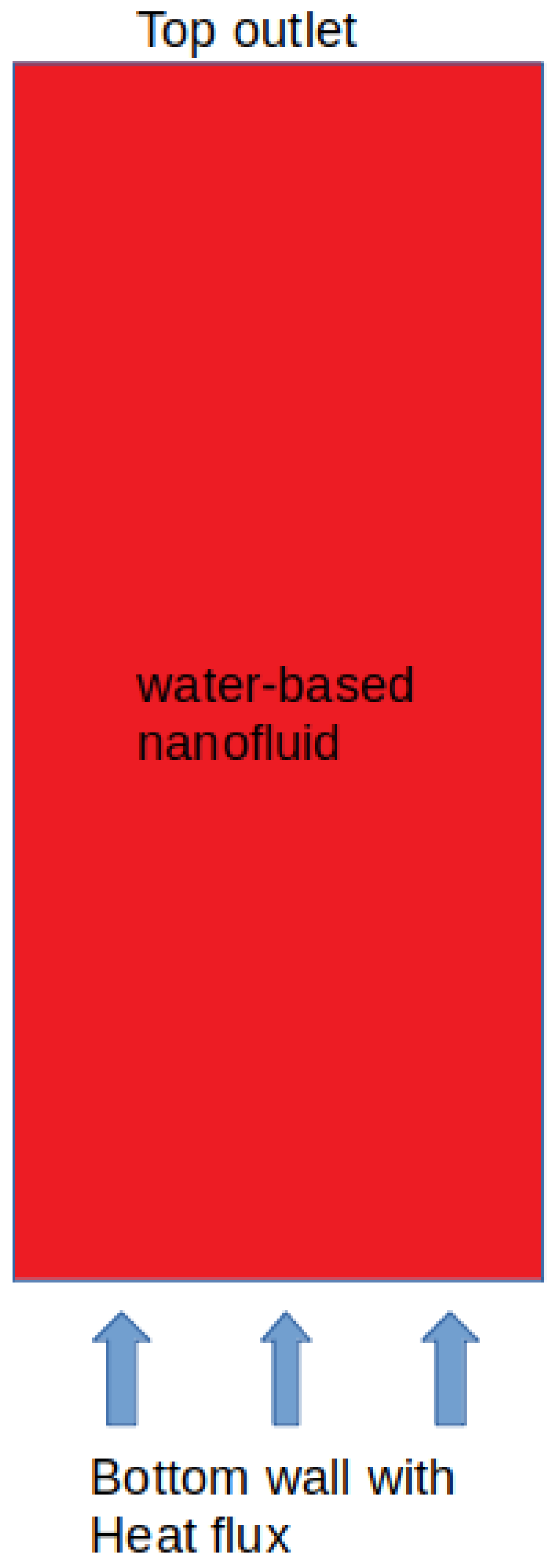
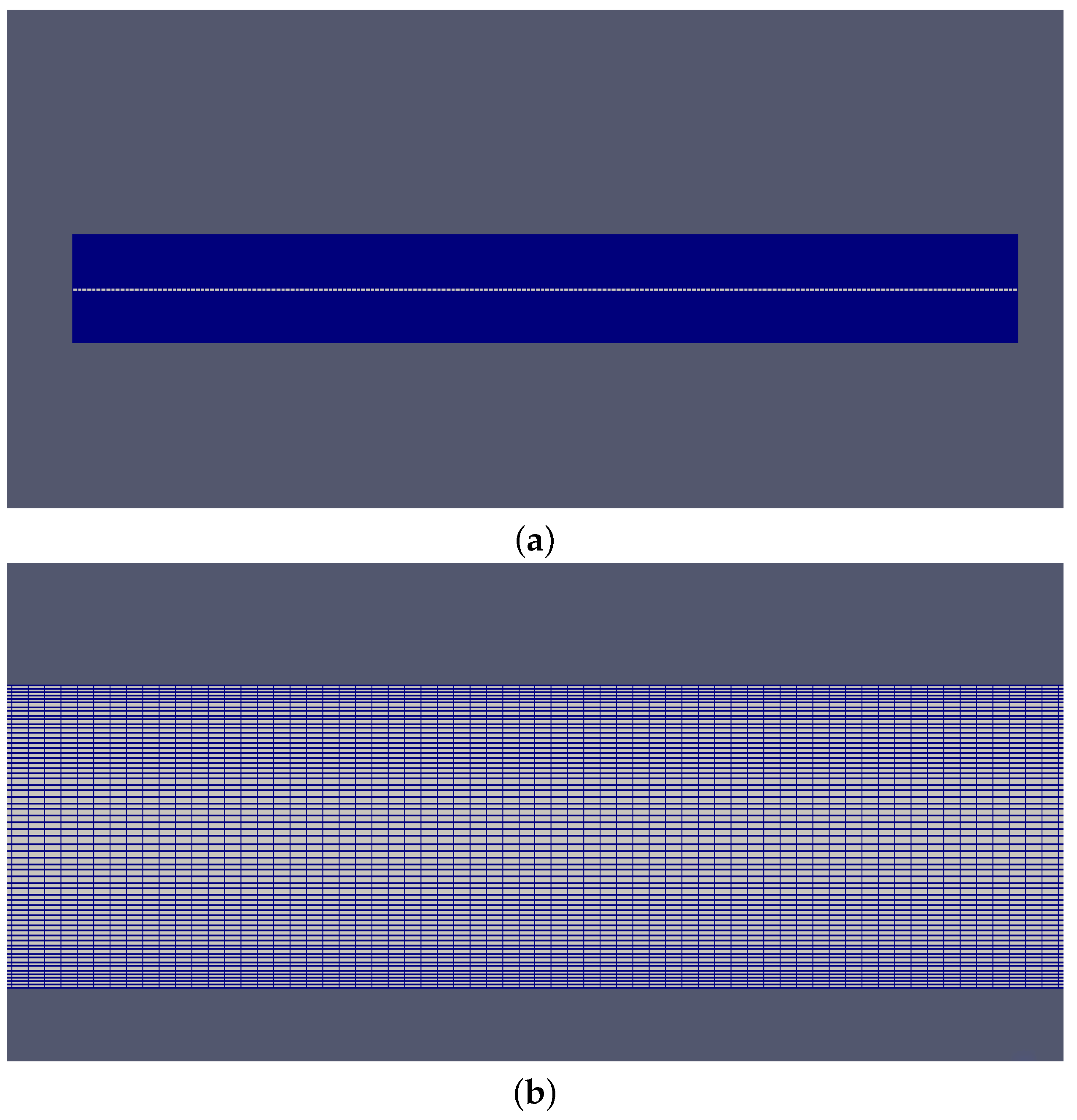
The physical model geometry is represented by a vertical rectangular channel of vertical length 4 m and horizontal width 1 m, see illustration in Figure 1. The fluid flow is in the upward-direction, with fluid entering at the bottom and exiting out the top.

The computational modelling in the present two-phase, liquid-gas flow study will require an efficient method to continuously track (in space and time) the liquid-vapour interface. The well developed volume-of-fluid (VOF) method will be employed for these purposes – to track the liquid-vapour interface. Specifically, the VOF method uses a volume-fraction indicator, say $\alpha$, to describe the volume-fraction of one phase (say the liquid phase) at any point and time in a computational cell within the flow field [34]. The volume-fraction $\alpha$ in the present sense will therefore be taken to indicate the ratio of the liquid volume in a computational cell to the total cell volume. It therefore easily follows that if the cell is completely filled with liquid, then $\alpha =1$, if the cell is completely filled with vapour, then $\alpha =0$, if the cell is half filled with liquid, then $\alpha =0.5$, if the cell is three quarter filled with liquid, then $\alpha =0.75$, etc. This leads to the following definition of the volume-fraction $\alpha$

$$\begin{array}{c}\hfill \alpha (y,t)=\left\{\begin{array}{cc}0& \mathrm{vapour}\mathrm{phase},\\ 0<\alpha <1& \mathrm{mixing}\mathrm{region},\\ 1& \mathrm{liquid}\mathrm{phase}.\end{array}\right.\end{array}$$

The flow quantities, i.e., the density ($\rho$), heat capacity ($c_p$), viscosity ($\mu$), and thermal conductivity (K), of the three-phase mixture may therefore be computed, in each computational cell, as the linear combinations of the respective contributions from the nanofluid phase, ${\left(\right)}_{nf}$, and the vapour phase, ${\left(\right)}_v$,

$$\begin{array}{c}\hfill \rho =\alpha {\rho }_{nf}+(1-\alpha ){\rho }_v,\end{array}$$

(1)

$$\begin{array}{c}\hfill \rho c_p=\alpha {\left(\rho c_p\right)}_{nf}+(1-\alpha ){\left(\rho c_p\right)}_v,\end{array}$$

(2)

$$\begin{array}{c}\hfill \mu =\alpha {\mu }_{nf}+(1-\alpha ){\mu }_v,\end{array}$$

(3)

$$\begin{array}{c}\hfill K=\alpha K_{nf}+(1-\alpha )K_v,\end{array}$$

(4)

where, ${\left(\right)}_{nf}$, represents the homogeneous nanofluid mixture formed from the combination of solid nano-particles, ${\left(\right)}_s$, that are homogeneously embedded in the base-liquid, ${\left(\right)}_{bl}$, phase. What we have so far referred to as the liquid-phase, should therefore more correctly now be referred to as the base-liquid phase. Specifically, the three-phase mixture is composed of nano-particles, a base-liquid, and a vapour. The nano-particles and base-liquid are homogeneously mixed to form the nanofluid.

The nanofluid density, heat capacity, and viscosity are calculated from a combination of the solid (nano-particle) contribution, ${\left(\right)}_s$, and the base-liquid contribution, ${\left(\right)}_{bl}$, see for example [33,35,36,37,38],

$$\begin{array}{c}\hfill {\rho }_{nf}=\phi {\rho }_s+(1-\phi ){\rho }_{bl},\end{array}$$

(5)

$$\begin{array}{c}\hfill {\left(\rho c_p\right)}_{nf}=\phi {\left(\rho c_p\right)}_s+(1-\phi ){\left(\rho c_p\right)}_{bl},\end{array}$$

(6)

$$\begin{array}{c}\hfill {\mu }_{nf}=\frac{{\mu }_{bl}}{{\left(\sqrt{1-\phi }\right)}^5}.\end{array}$$

(7)

where $\phi \in [0,1]$ is the volume-fraction of the nano-particles,

$$\begin{array}{c}\hfill \phi =\left\{\begin{array}{cc}0,& 0\%\mathrm{of}\mathrm{nano}\text{-}\mathrm{particles}\mathrm{by}\mathrm{volume}\mathrm{in}\mathrm{nanofluid},\hfill \\ 0<\phi <1,& 100\phi \%\mathrm{nano}\text{-}\mathrm{particles}\mathrm{by}\mathrm{volume}\mathrm{in}\mathrm{nanofluid},\hfill \\ 1,& 100\%\mathrm{nano}\text{-}\mathrm{particles}\mathrm{by}\mathrm{volume}\mathrm{in}\mathrm{nanofluid}.\hfill \end{array}\right.\end{array}$$

The thermal conductivity for the nanofluid is empirically determined, see for example [33,35,36,37,38]. The following empirical formula is adopted,

$$\begin{array}{c}\hfill K_{nf}=\frac{K_s+(1-\aleph )K_{bl}+(1-\aleph )\phi (K_{bl}-K_s)}{K_s+(1-\aleph )K_{bl}+\phi (K_{bl}-K_s)}(1+\epsilon A_{2}T),\end{array}$$

(8)

where $\epsilon$ and $A_2$ are thermal-conductivity parameters and ℵ is an empirically determined nano-particle shape-factor. For spherical-shaped nano-particles, $\aleph =3$, [33,35,36,37,38].

2.1. Conservation Equations

The dynamical governing equations for the nanofluid and vapour phases are obtained from the conservation laws, namely the conservation of mass, momentum, and energy, respectively given as,

$$\begin{array}{cc}\hfill & \frac{\partial \rho }{\partial t}+\nabla ·\left(\rho \mathit{U}\right)=0,\hfill \\ \hfill & \hfill \end{array}$$

(9)

$$\begin{array}{cc}\hfill & \frac{\partial }{\partial t}\left(\rho \mathit{U}\right)+\nabla ·\left(\rho \mathit{U}\mathit{U}\right)=-\nabla p+\nabla ·\left[\mu (\nabla \mathit{U}+\nabla {\mathit{U}}^T)-\frac{2}{3}(\nabla ·\mathit{U})\mathit{I}\right]+\rho ({\mathit{F}}_g+{\mathit{F}}_{\sigma }),\hfill \\ \hfill & \hfill \end{array}$$

(10)

$$\begin{array}{cc}\hfill & \frac{\partial }{\partial t}\left(\rho c_{p}T\right)+\mathit{U}·\nabla \left(\rho c_{p}T\right)=\nabla ·(K\nabla T)+Q,\hfill \end{array}$$

(11)

where $\rho$ is the fluid density, t is time, $\mathit{U}$ the velocity field, p the pressure field, ${\mathit{F}}_g$ is the gravitational force field, ${\mathit{F}}_{\mathbf{\sigma }}$ is the force due to surface-tension, T the temperature field, $\mathit{I}$ is the unit tensor, $c_p$ the specific heat capacity at constant pressure, K is the thermal conductivity, and Q represents heat sources. The surface-tension, ${\mathit{F}}_{\sigma }$, is calculated using the continuum-surface-force (CSF) model for the cells containing the nanofluid-vapour interface [18,39],

$${\displaystyle {\mathit{F}}_{\sigma }=\sigma \frac{{\rho }_{nf}{\alpha }_{nf}{\kappa }_v{\mathit{N}}_v+{\rho }_v{\alpha }_v{\kappa }_{nf}{\mathit{I}}_{nf}}{0.5\left({\rho }_{nf}+{\rho }_v\right)},}$$

(12)

where $\sigma$ is the surface tension of the nanofluid, ${\alpha }_v$ is the vapour volume fraction, ${\alpha }_{nf}$ is the nanofluid volume fraction, ${\rho }_v$ is the vapour density, ${\rho }_{nf}$ is the nanofluid density, ${\kappa }_v$ is the curvature of the vapour phase, ${\kappa }_{nf}$ is the curvature of the nanofluid phase. In our notation, we assume ${\alpha }_{nf}=\alpha$ and ${\alpha }_v=1-{\alpha }_{nf}=1-\alpha$. The unit normal vectors are defined as,

$${\mathit{N}}_{nf}=\frac{\nabla {\alpha }_{nf}}{\nabla {\alpha }_{nf}},{\mathit{N}}_v=\frac{\nabla {\alpha }_v}{\nabla {\alpha }_v}.$$

(13)

In the Lee model, [24], which is adopted in the present work, the continuity (mass conservation) equation, Equation (9), is not solved directly for the combined phases, as with the momentum and energy equations, Equations (10) and (11). The mass conservation equation will therefore be solved, for each phase, via Lee’s phase change model.

2.2. Phase Change Model

The phase change model is described via Lee’s model [24]. This model is based on the assumption that mass is transferred at a quasi-thermo-equilibrium and at constant pressure. The mass transfer depends mainly on the shared and saturated temperatures. Accordingly, the mass conservation equations for the volume fractions of the nanofluid and vapour phases are respectively,

$$\begin{array}{cc}\hfill \frac{\partial {\alpha }_{nf}}{\partial t}+\nabla ·\left(\mathit{U}{\alpha }_{nf}\right)& =\frac{S_{nf}}{{\rho }_{nf}},\hfill \end{array}$$

(14)

$$\begin{array}{cc}\hfill \frac{\partial {\alpha }_v}{\partial t}+\nabla ·\left(\mathit{U}{\alpha }_v\right)& =\frac{S_v}{{\rho }_v}.\hfill \end{array}$$

(15)

The source terms due to phase change, $S_{nf}$ and $S_v$ are adopted from Lee’s phase change model [24],

$$\begin{array}{cc}\hfill S_{nf}& =C_{nf}{\rho }_{nf}{\alpha }_{nf}{\rho }_{nf}\frac{T-T_{\mathrm{sat}}}{T_{\mathrm{sat}}}T\ge T_{\mathrm{sat}},\hfill \end{array}$$

(16)

$$\begin{array}{cc}\hfill S_v& =C_v{\rho }_v{\alpha }_v{\rho }_v\frac{T_{\mathrm{sat}}-T}{T_{\mathrm{sat}}}T<T_{\mathrm{sat}},\hfill \end{array}$$

(17)

where $T_{\mathrm{sat}}$ is the saturation temperature of the nanofluid, T is the temperature of the three-phase mixture, $C_{nf}$ and $C_e$ are empirically determined phase change coefficients [1,27,40,41]. The values of C must be chosen such that they maintain the interfacial temperature reasonably close to the saturation temperature and also prevent divergence problems. We adopt the value $C=C_{nf}=C_v=1500$ s${}^{-1}$ used in [24].

2.3. Turbulence Modelling

The turbulence modelling is achieved via the Shear Stress Transport (SST) model, see [42,43], which essentially combines the best aspects of the k-$\omega$ and the k-$\epsilon$ formulations,

$$\begin{array}{cc}\hfill \frac{D}{Dt}\left(\rho k\right)& =\mathbf{\Sigma }-{\beta }^{*}\rho k\omega +\nabla ·[(\mu +{\sigma }_k{\mu }_t)\nabla k]\hfill \\ \hfill & \hfill \end{array}$$

(18)

$$\begin{array}{cc}\hfill \frac{D}{Dt}\left(\rho \omega \right)& =\frac{\gamma }{\widehat{{\nu }_t}}\widehat{\mathbf{\Sigma }}-\beta \rho {\omega }^2+\nabla ·[(\mu +{\sigma }_{\omega }{\mu }_t)\nabla \omega ]+2(1-F1)\rho {\sigma }_{\omega 2}\frac{1}{\omega }\nabla k·\nabla \omega .\hfill \end{array}$$

(19)

The production terms, $\mathbf{\Sigma }$ and $\widehat{\mathbf{\Sigma }}$, are,

$$\begin{array}{cc}\hfill \widehat{\mathbf{\Sigma }}& =\left[{\mu }_t\left(\nabla \mathit{U}+{\nabla \mathit{U}}^T-\frac{2}{3}(\nabla ·\mathit{U})\mathit{I}\right)-\frac{2}{3}\rho k\mathit{I}\right]\nabla \mathit{U},\hfill \\ \hfill & \hfill \end{array}$$

(20)

$$\begin{array}{cc}\hfill \mathbf{\Sigma }& =min\{\widehat{\mathbf{\Sigma }},10{\beta }^{*}\rho k\omega \},\hfill \end{array}$$

(21)

where $\mathit{I}$ is the unit tensor. The kinematic eddy viscosities are,

$$\begin{array}{cc}\hfill {\nu }_t& =\frac{{\mu }_t}{\rho }=\frac{a_{1}k}{max\{a_1\omega ,\dot{\gamma }{F}_2\}},\hfill \\ \hfill & \hfill \end{array}$$

(22)

$$\begin{array}{cc}\hfill \widehat{{\nu }_t}& =max\{{\nu }_t,{10}^{-8}\},\hfill \end{array}$$

(23)

where $\dot{\gamma }$ is the invariant measure of the rate-of-strain, i.e., the absolute value of the strain rate,

$$\dot{\gamma }=\mathit{S}=\sqrt{2\mathit{S}:{\mathit{S}}^T},\mathrm{where}\mathit{S}=\frac{1}{2}\left[\nabla \mathit{U}+{(\nabla \mathit{U})}^T\right].$$

(24)

The material derivative $D/Dt$ is,

$$\frac{D}{Dt}\left(\rho \omega \right)=\frac{\partial \rho \omega }{\partial t}+\mathit{U}·\nabla \left(\rho \omega \right),$$

(25)

For ease of comparison with the notation of [42,43], Equations (18) and (19) may also be cast in tensorial index notation, for example, Equation (18) can be recast as,

$$\begin{array}{c}\hfill \frac{\partial }{\partial t}\left(\rho k\right)+\frac{\partial }{\partial x_i}\left(\rho U_{i}k\right)={\Sigma }_k-{\beta }^{*}\rho k\omega +\frac{\partial }{\partial x_i}\left[(\mu +{\sigma }_k{\mu }_t)\frac{\partial k}{\partial x_i}\right],\end{array}$$

(26)

with,

$$\begin{array}{cc}\hfill {\widehat{\Sigma }}_k& =\left[{\mu }_t\left(U_{i,j}+U_{j,i}-\frac{2}{3}\nabla ·U_{k,k}{\delta }_{ij}\right)-\frac{2}{3}\rho k{\delta }_{ij}\right]U_{i,j},\hfill \\ \hfill & \hfill \end{array}$$

(27)

$$\begin{array}{cc}\hfill {\Sigma }_k& =min\{{\widehat{\Sigma }}_k,10{\beta }^{*}\rho k\omega \},\hfill \end{array}$$

(28)

The blending functions, $F_1$ and $F_2$, are similarly defined as in [42,43],

$$\begin{array}{cc}\hfill F_1& =tanh\left\{{\left\{min\left[max\left(\frac{\sqrt{k}}{{\beta }^{*}\omega Y},\frac{500\nu }{Y^2\omega }\right),\frac{4\rho {\sigma }_{\omega 2}k}{{\mathrm{CD}}_{k\omega }{Y}^2}\right]\right\}}^4\right\},\hfill \end{array}$$

(29)

$$\begin{array}{cc}\hfill F_2& =tanh\left[{\left[max\left(\frac{2\sqrt{k}}{{\beta }^{*}\omega Y},\frac{500\nu }{Y^2\omega }\right)\right]}^2\right],\hfill \end{array}$$

(30)

where the closure coefficient, ${\mathrm{CD}}_{k\omega }$, is defined as,

$${\mathrm{CD}}_{k\omega }=max\left(2\rho {\sigma }_{\omega 2}\frac{1}{\omega }\nabla k·\nabla \omega ,{10}^{-10}\right).$$

(31)

In index tensor notation, we can write,

$$\nabla k·\nabla \omega =\frac{\partial k}{\partial x_i}\frac{\partial \omega }{\partial x_i}.$$

(32)

The coefficients embedded in the SST model are calculated from the blending function, $F_1$, using formulas such as,

$$\beta =F_1{\beta }_1+(1-F_1){\beta }_2,\gamma =F_1{\gamma }_1+(1-F_1){\gamma }_2,\mathrm{etc}.$$

(33)

where ${\left(\right)}_1$ and ${\left(\right)}_2$ represent the coefficients of the k-$\omega$ and the k-$\epsilon$ model respectively. The values of these coefficients are given in [42,43],

$$\begin{array}{cc}\hfill k\text{-}\omega :& {\sigma }_{k_1}=1.176,{\sigma }_{{\omega }_1}=2.000,\kappa =0.41,{\gamma }_1=0.5532,{\beta }_1=0.0750,{\beta }^{*}=0.09,c_l=10,\hfill \\ \hfill k\text{-}\epsilon :& {\sigma }_{k_2}=1.000,{\sigma }_{{\omega }_2}=1.168,\kappa =0.41,{\gamma }_2=0.4403,{\beta }_2=0.0828,{\beta }^{*}=0.09.\hfill \end{array}$$

3. Numerical and Computational Methodologies

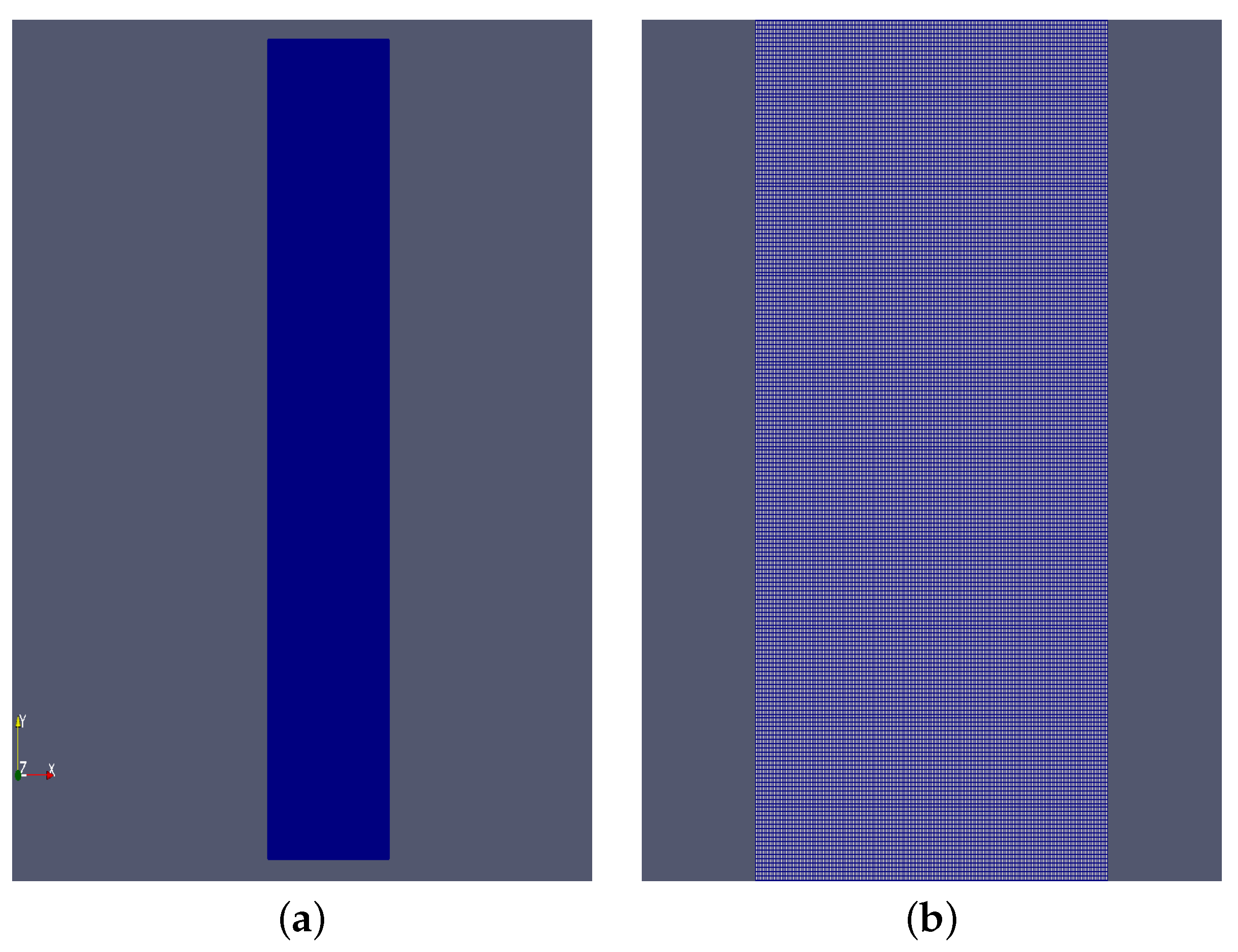
The computational domain and 2D uniform mesh used in the simulations are respectively shown in Figure 2a,b. The computational mesh grid is created using the OpenFOAM mesh generation tool, blockMesh.

The OpenFOAM software implements finite volume methods (FVM) as the standard numerical methodology for the solution of governing equations. The interCondensatingEvaporatingFoam solver which already exists on the OpenFOAM platform is designed for two-phase, liquid-gas, boiling flow simulations. This solver is adopted and modified as necessary to fit the simulations in the present work, specifically, the inclusion of the solid (nano-particle) phase and hence also incorporating relevant modifications to the embedded parameters such as the base-liquid density, viscosity, specific heat capacity, and thermal conductivity.

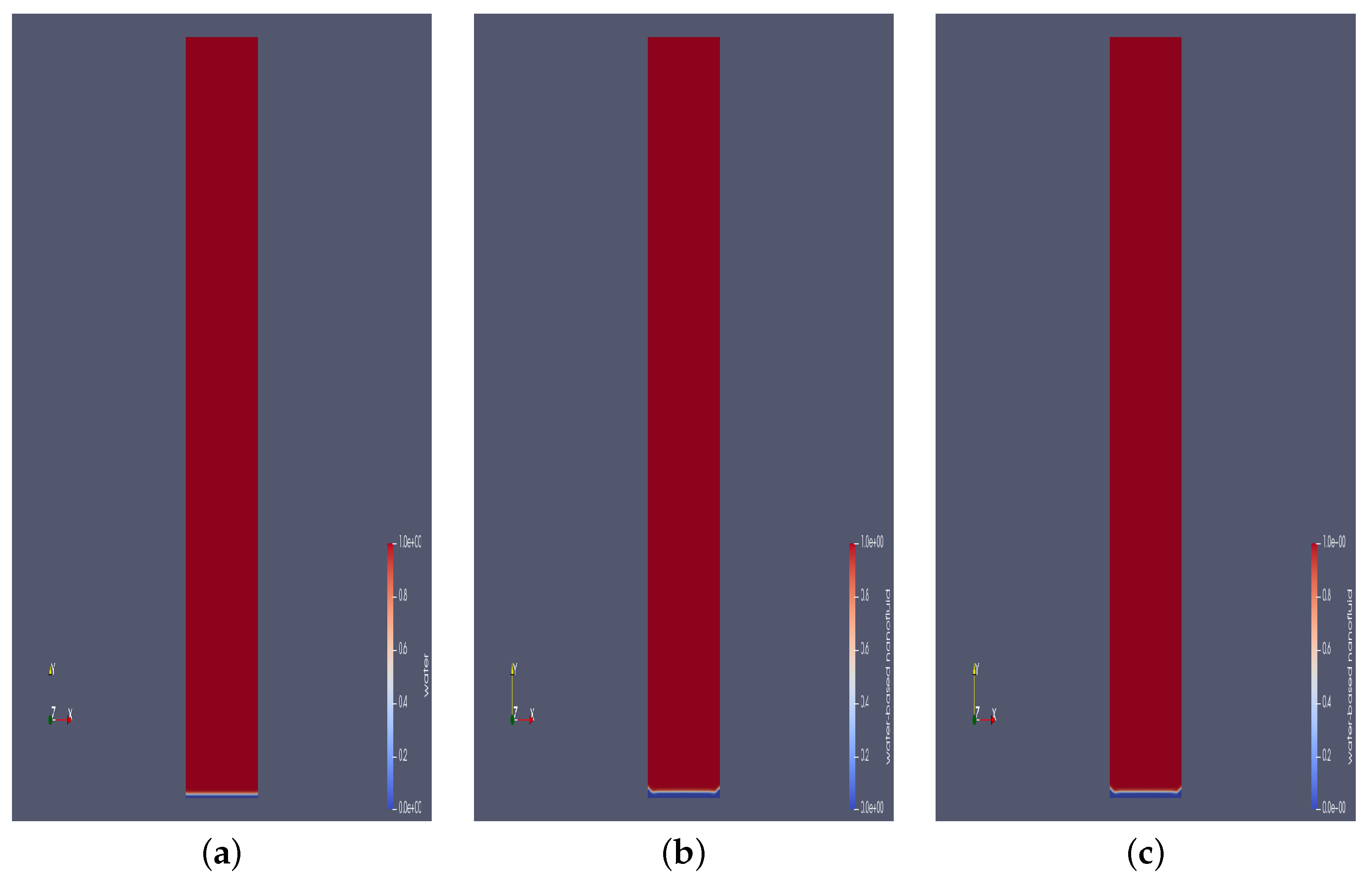
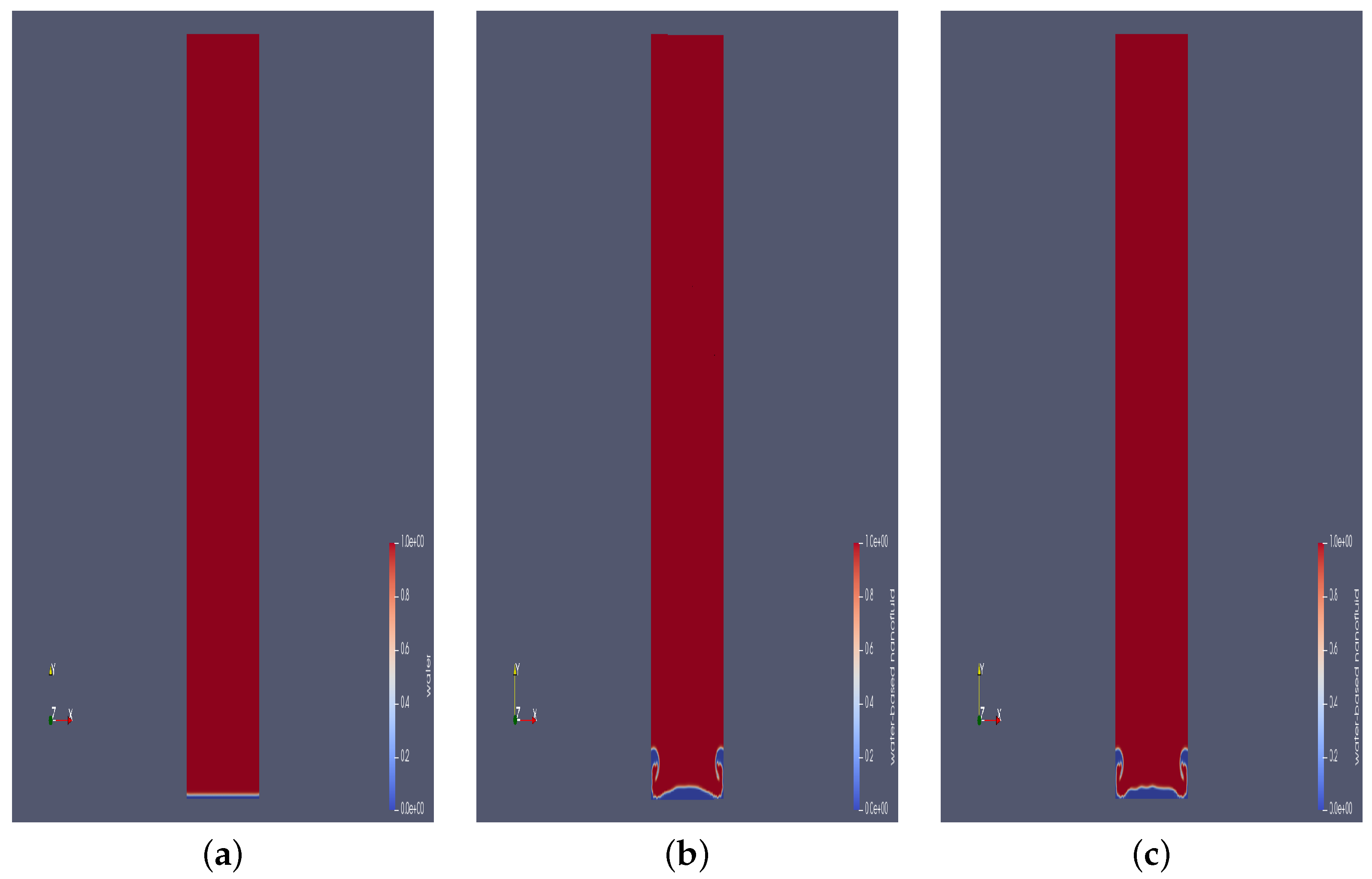
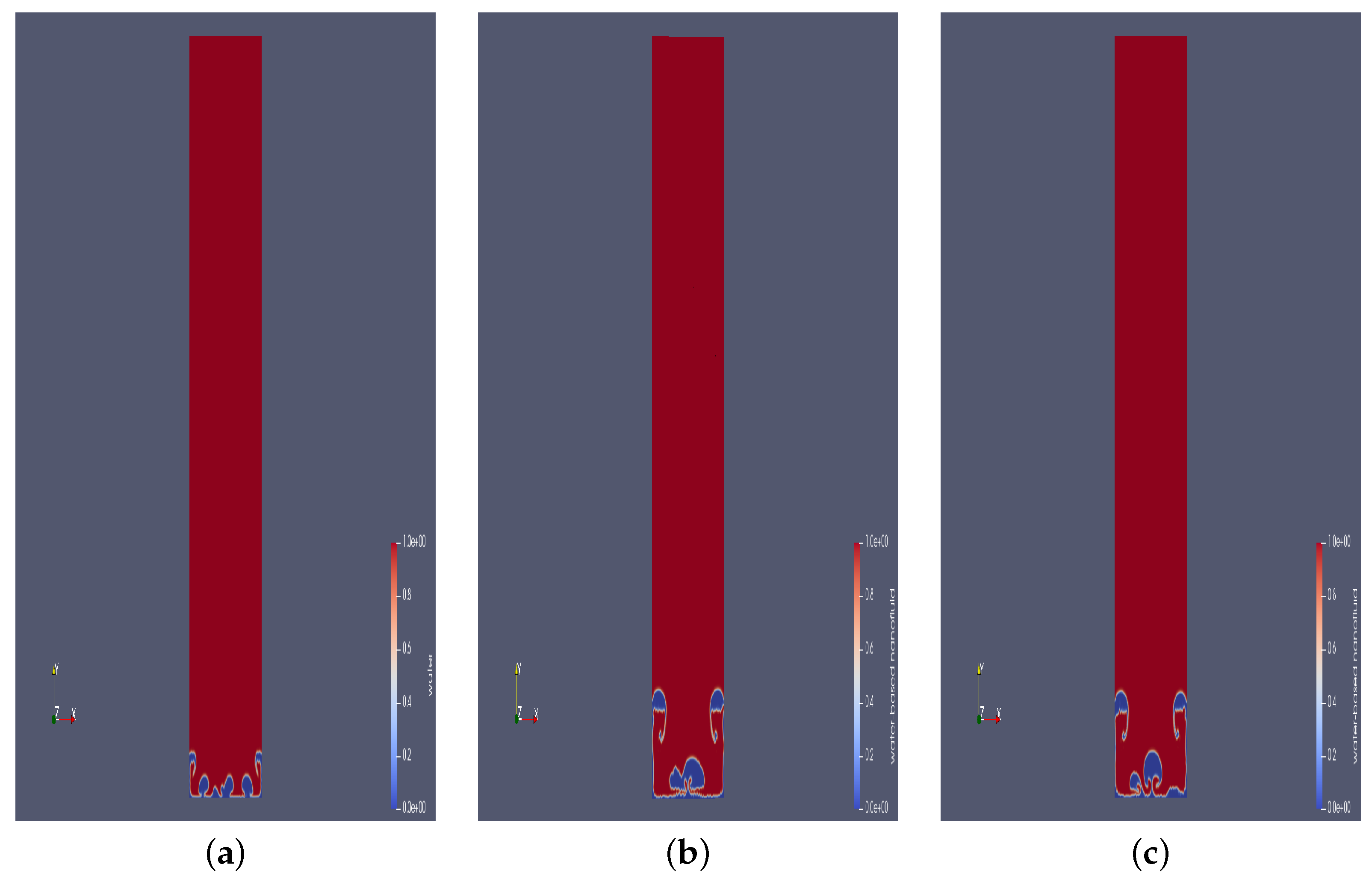
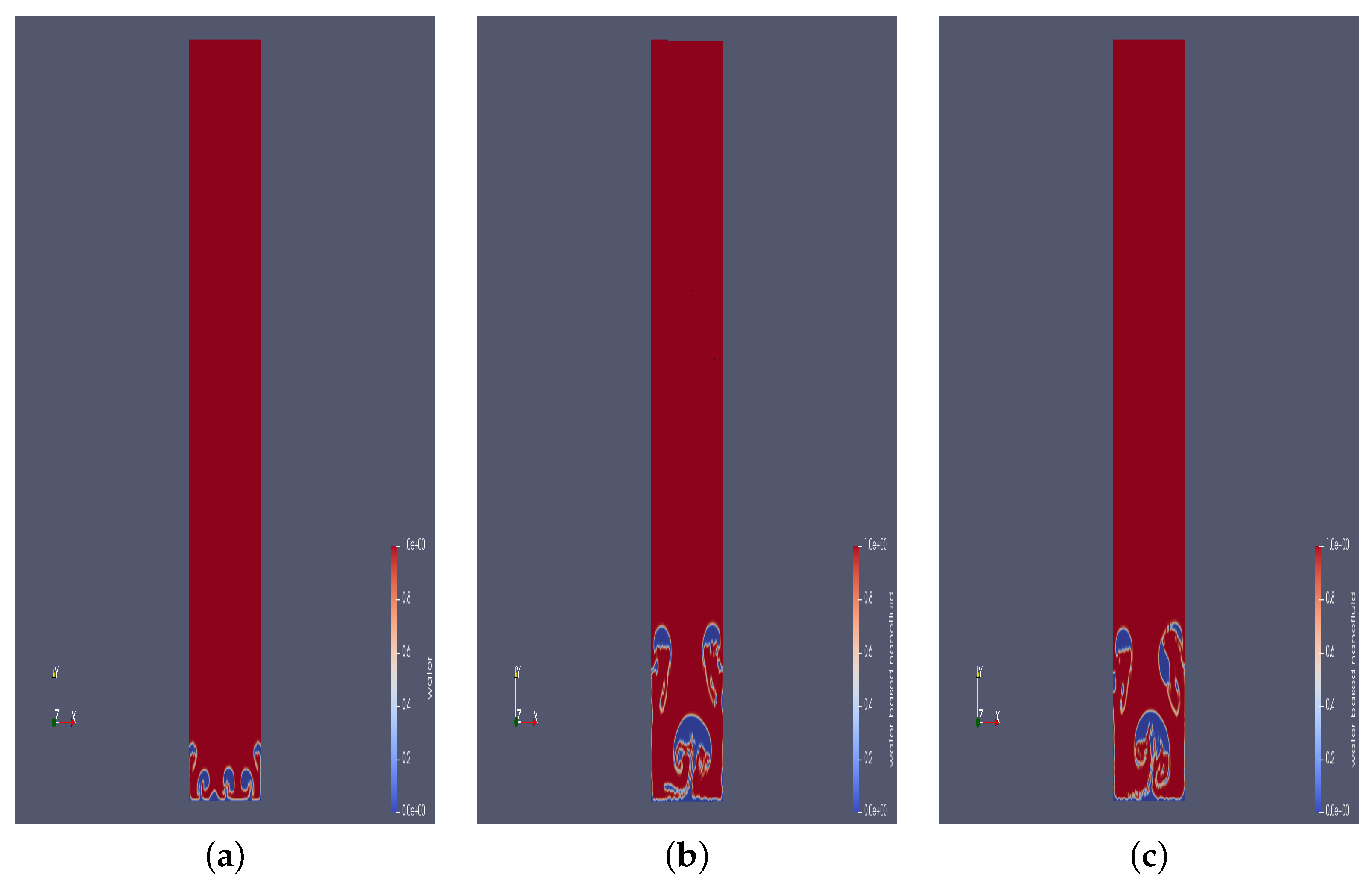
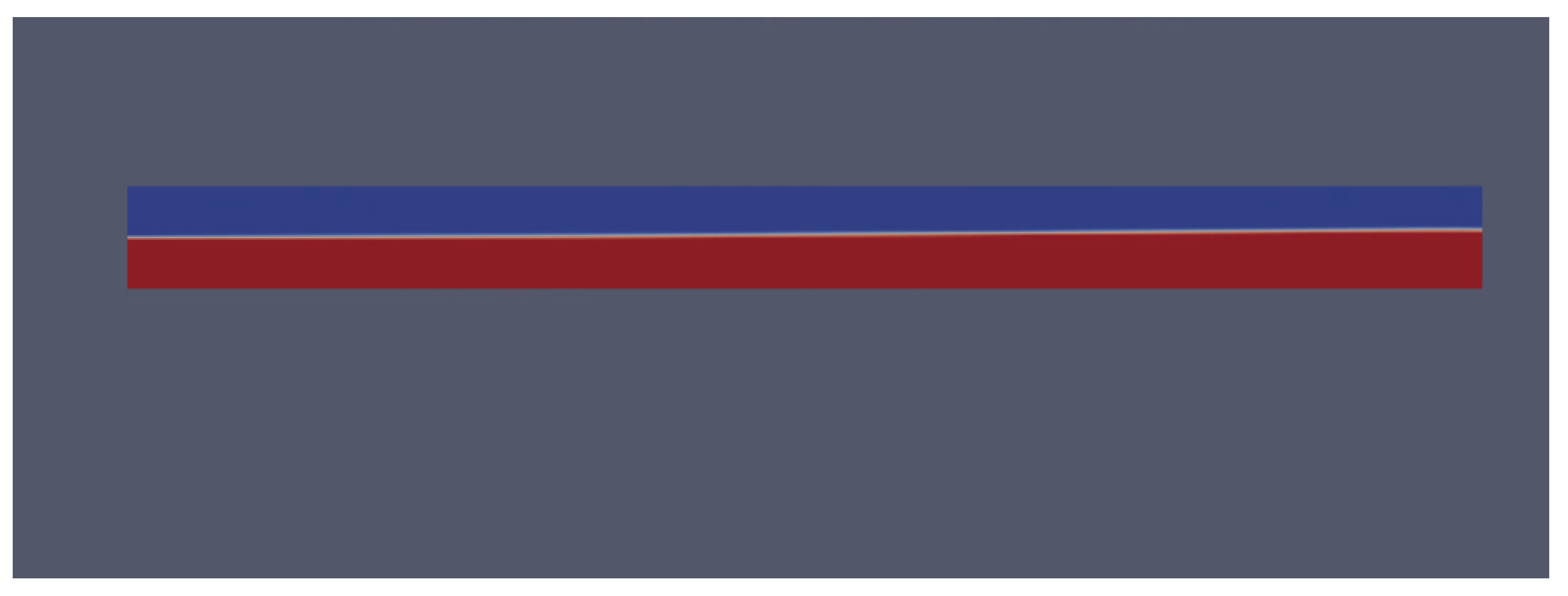
The multi-phase mixture is initially at rest (at time $t<0$) with an initial temperature of 373 K and pressure at ${10}^5$ kg/m${}^3$. The turbulence parameters, $k,\epsilon ,{\nu }_t$, and $\omega$ are all set to 1. At the bottom wall, the temperature is set at 390 K and the velocity is maintained at 0 m/s. The subsequent motion of fluid in the channel is entirely attributed to convective heat fluxes as a result of the heat flux introduced at the bottom wall from time $t\ge 0$. Standard no-slip boundary conditions are imposed on the velocity at the vertical (solid) walls. The wall function boundary condition is implemented for the turbulence parameters. The inlet-outlet boundary condition is also implemented for turbulence parameters except for ${\nu }_t$ for which a calculated boundary condition is used. At the outlet, zero-gradient boundary conditions are considered for temperature and velocity while a calculated boundary condition is used for the pressure.

The pressure-velocity coupling is resolved via the PIMPLE algorithm, a combination of the Pressure Implicit with Splitting of Operator (PISO) and the Semi-Implicit Method for Pressure-Linked Equations (SIMPLE) algorithms. A combination of Gauss linear, Gauss upwind, and Gauss interface compression are used for the discretization of spatial derivatives. The first order implicit Euler method is used for the discretization of time derivatives. The discrete systems of algebraic equations are solved via robust linear algebraic techniques with appropriate smoothers. A symmetric Gauss-Seidel smoother is employed for the temperature, velocity, and pressure equations. The pressure equation is otherwise solved via the Preconditioned-Conjugate-Gradient (PCG) technique in conjunction with Geometric-Algebra-Multi-Grid (GAMG) and Diagonal-Incomplete-Cholesky (DIC) pre-conditioners. Turbulence equations are solved using the Preconditioned Bi-Conjugate Gradient Stabilized (PBiCGStab) solver with a Diagonal-Incomplete-LU (DILU) pre-conditioner.

4. Results and Discussion

Unless otherwise indicated, the default values for the embedded flow quantities as displayed in Table 1, Table 2, Table 3 and Table 4 will be assumed in the subsequent analysis.

• General quantities:

Table 1. Default values for general flow quantities.

Number of computational cells (${\mathit{M}}_1$)	100,000 cells
Final computational time	10 s
Volume fraction ($\phi$)	$0.2$
Initial fluid temperature	373 K for $t<0$
Bottom wall fluid temperature	390 K for $t\ge 0$
Initial fluid velocity	0 m/s throughout channel
Initial fluid pressure	${10}^5$ kg/m${}^3$

Table 1. Default values for general flow quantities.

Number of computational cells (${\mathit{M}}_1$)	100,000 cells
Final computational time	10 s
Volume fraction ($\phi$)	$0.2$
Initial fluid temperature	373 K for $t<0$
Bottom wall fluid temperature	390 K for $t\ge 0$
Initial fluid velocity	0 m/s throughout channel
Initial fluid pressure	${10}^5$ kg/m${}^3$

• Water, H${}_{\mathbf{2}}$O:

Table 2. Default values for water.

Viscosity of water	0.001 kg/m/s
Density of water	997.10 kg/m${}^3$
Specific heat for water	4180 J/K/kg
Thermal conductivity for water	0.6071 W/m/K

Table 2. Default values for water.

Viscosity of water	0.001 kg/m/s
Density of water	997.10 kg/m${}^3$
Specific heat for water	4180 J/K/kg
Thermal conductivity for water	0.6071 W/m/K

• Aluminium Oxide (Al${}_{\mathbf{2}}$O${}_{\mathbf{3}}$) nano-particles:

Table 3. Default values for Aluminium Oxide.

Density of Al${}_2$O${}_3$ nano-particles	3970 kg/m${}^3$
Specific heat for Al${}_2$O${}_3$ nano-particles	765 J/K/kg
Thermal conductivity for Al${}_2$O${}_3$ nano-particles	40 W/m/K

Table 3. Default values for Aluminium Oxide.

Density of Al${}_2$O${}_3$ nano-particles	3970 kg/m${}^3$
Specific heat for Al${}_2$O${}_3$ nano-particles	765 J/K/kg
Thermal conductivity for Al${}_2$O${}_3$ nano-particles	40 W/m/K

• Titanium Oxide (TiO${}_{\mathbf{2}}$) nano-particles:

Table 4. Default values for Titanium Oxide.

Density of TiO${}_2$ nano-particles	4250 kg/m${}^3$
Specific heat for TiO${}_2$ nano-particles	686.2 J/K/kg
Thermal conductivity for TiO${}_2$ nano-particles	8.9538 W/m/K

Table 4. Default values for Titanium Oxide.

Density of TiO${}_2$ nano-particles	4250 kg/m${}^3$
Specific heat for TiO${}_2$ nano-particles	686.2 J/K/kg
Thermal conductivity for TiO${}_2$ nano-particles	8.9538 W/m/K

4.1. Mesh Dependence

Unlike laminar flows for which reproducible steady-state solutions would be expected after a certain time, turbulent flows are not expected to settle to reproducible steady states. In other words, time convergence to reproducible (identical) steady-state solutions would not be expected for turbulent flow. Even though the quantitative solutions would be expected to differ as indicated, the qualitative behaviour of the turbulent flow solutions would still be expected to be similar. Figure 3 gives the results obtained from using three different mesh sizes; $M_1,M_2,M_3$; and as expected, the quantitative solutions are different but the qualitative behaviour is similar.

4.2. Numerical Validation—Two-Phase Flow

To validate the efficacy of the numerical and computational methodologies employed in this investigation, the well documented two-phase, water-air, boiling flow problem in a horizontal channel is considered. The various flow patterns for such two-phase, water-air, boiling flow in a rectangular horizontal channel are illustrated in Figure 4 which is adapted from [44].

The 2D horizontal channel and corresponding mesh used in the validation tests are shown in Figure 5a,b, respectively. The mesh grid is generated via the OpenFOAM mesh generation tool, blockMesh.

The computational results obtained using the numerical approaches of the present investigation, as displayed in Figure 6, Figure 7, Figure 8 and Figure 9 respectively, replicate the expected flow patterns, shown in Figure 4 which is adapted from [44], corresponding to stratified flow, way flow, plug flow, and bubbly flow.

4.3. Nanofluid Results

The transient results, illustrating the evolution in time of the flow patterns for the three types of multi-phase fluid-mixtures, namely; a two-phase water-vapour mixture; a water-vapour-Al${}_2$O${}_3$ nanofluid mixture; and a water-vapour-TiO${}_2$ are shown in Figure 10, Figure 11, Figure 12 and Figure 13.

The computational results shown in Figure 10, Figure 11, Figure 12 and Figure 13 are able to accurately simulate the boiling process and to subsequently capture the formation of vapour bubbles as time progresses. As time progresses, the hotter fluid progressively becomes dominant leading to boiling and the formation of vapour bubbles. The results demonstrate that the boiling process, and hence also formation of vapour bubbles (denoted by the blue areas in the graphs), is significantly enhanced for the nanofluid cases than for the ordinary water case. The bubbly regions are identified by the regions of low temperature, i.e., the blue areas on the graphs. The explanation for this is straightforward. The region inside the air/vapour bubbles will always be significantly cooler than that in the surrounding continuum liquid (water in this case). Plumbers generally use this simple test in domestic and industrial applications to check the flow properties and heating efficiencies of domestic or industrial geysers. By placing your hand under a tap of running hot water, if there is a significant presence of bubbles, then the water would not be as hot as expected from (or recorded on) the source-geyser thermostat settings.

The qualitative results for both types of nanofluids, H${}_2$O-Al${}_2$O${}_3$ nanofluid and H${}_2$O-TiO${}_2$, are similar despite the distinctly different properties of the constituent nano-particles. The reason reduces to the realization that the properties of the resultant nanofluids at the operating temperatures and volume fractions are in fact similar. This is illustrated in

Table 5. Comparative properties of water, nano-particles, and nanofluids at $T=390$ K and $\phi =0.2$.

	Al${}_2$O${}_3$	TiO${}_2$	H${}_2$O	H${}_2$O-Al${}_2$O${}_3$	H${}_2$O-TiO${}_2$
Density, kg/m${}^3$	3970	4250	997.10	1591.68	1647.68
Specific heat, J/K/kg	765	686.2	4180	3497	3481.24
Thermal conductivity, W/m/K	40	8.9538	0.6071	29.294551	30.295152

using the temperature, $T=390$ K, and the volume fraction, $\phi =0.2$.

Specifically, Table 5 shows that even though, say, the thermal conductivities of Al${}_2$O${}_3$ and TiO${}_2$ nano-particles are quite different—respectively 40 W/m/K and 8.9538 W/m/K—the respective thermal conductivities of the corresponding nanofluids, water-Al${}_2$O${}_3$ and water-TiO${}_2$, are practically similar—29.294551 W/m/K and 30.295152 W/m/K. These nanofluid thermal conductivities are significantly (nearly 50 times) higher than the corresponding thermal conductivity of water, 0.6071 W/m/K which explains the results in Figure 10, Figure 11, Figure 12 and Figure 13.

The results therefore clearly imply that the heat conduction properties, and hence also the boiling and bubble formation processes, may be enhanced by employing nanofluids of increasing nano-particle concentration. The results of Figure 14, Figure 15 and Figure 16, which are respectively for $\phi =0.05$, $\phi =0.1$, and $\phi =0.2$, provide the relevant confirmation.

As before, the qualitative results for both types of nanofluids, H${}_2$O-Al${}_2$O${}_3$ nanofluid and H${}_2$O-TiO${}_2$, are similar despite the distinctly different properties of the constituent nano-particles. As before, the reason reduces to the realization that the properties of the resultant nanofluids at the operating temperatures and volume fractions are in fact similar. This is illustrated in

Table 6. Comparative thermal-conductivities of water, nano-particles, and nanofluids at $T=390$ K.

	Al${}_2$O${}_3$	TiO${}_2$	H${}_2$O	H${}_2$O-Al${}_2$O${}_3$	H${}_2$O-TiO${}_2$
Thermal conductivity, $\phi =0.05$	40	8.9538	0.6071	19.264274	19.438368
Thermal conductivity, $\phi =0.1$	40	8.9538	0.6071	22.229736	22.619839
Thermal conductivity, $\phi =0.2$	40	8.9538	0.6071	29.294551	30.295152

using the temperature, $T=390$ K, and the volume fraction, $\phi =0.2$.

The results therefore clearly indicate that the thermal conductivities of the nanofluids, and hence also their corresponding heat conduction properties and hence also the boiling and bubble formation processes would be enhanced by increasing the concentration (volume fraction) of the embedded nano-particles. The results of Figure 14, Figure 15 and Figure 16; which are respectively for $\phi =0.05$, $\phi =0.1$, and $\phi =0.2$; provide the relevant confirmation.

5. Concluding Remarks

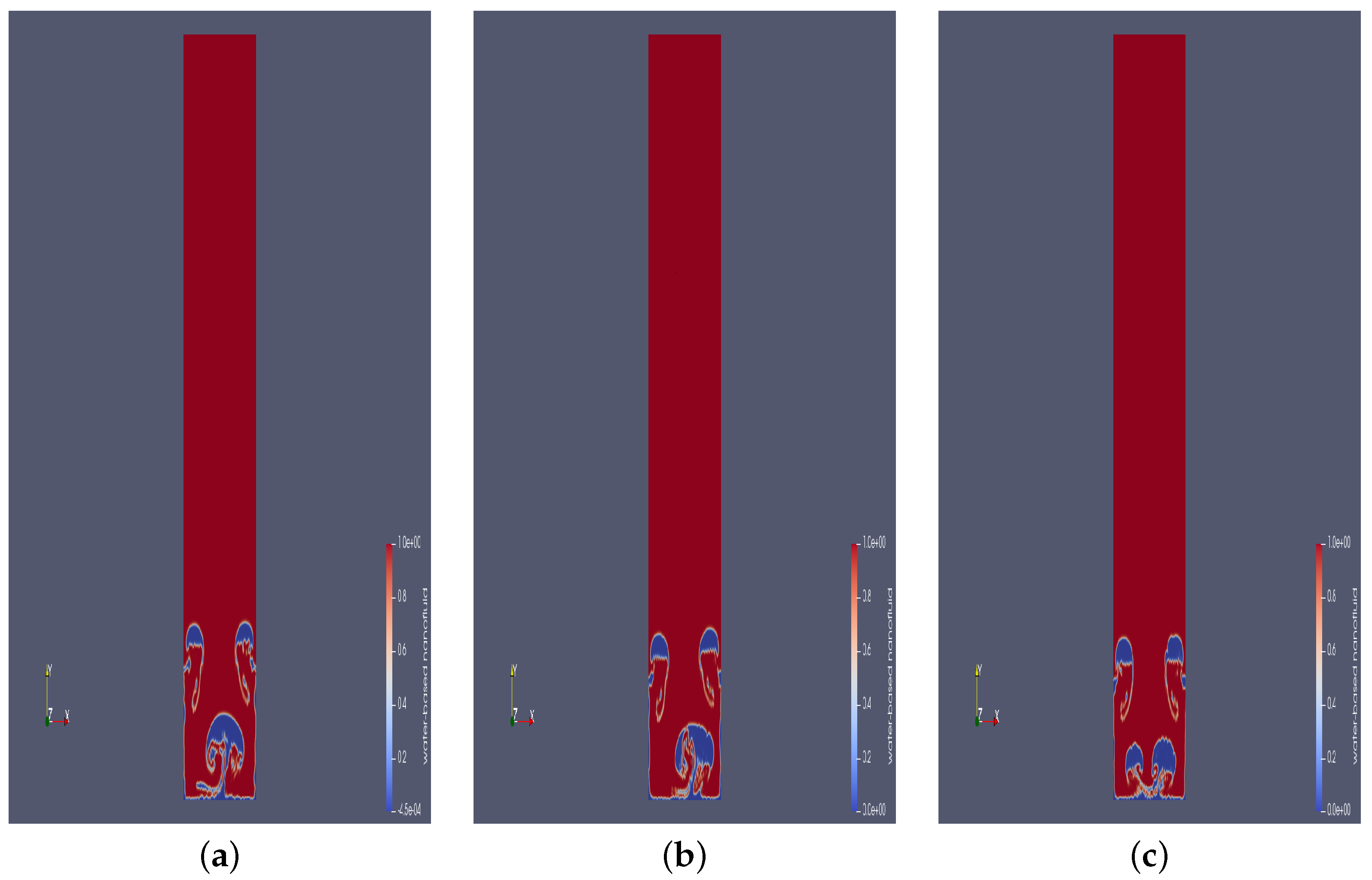
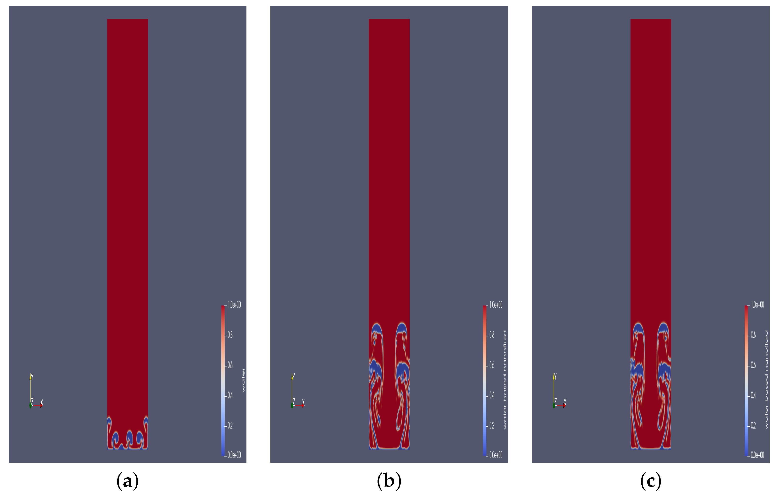
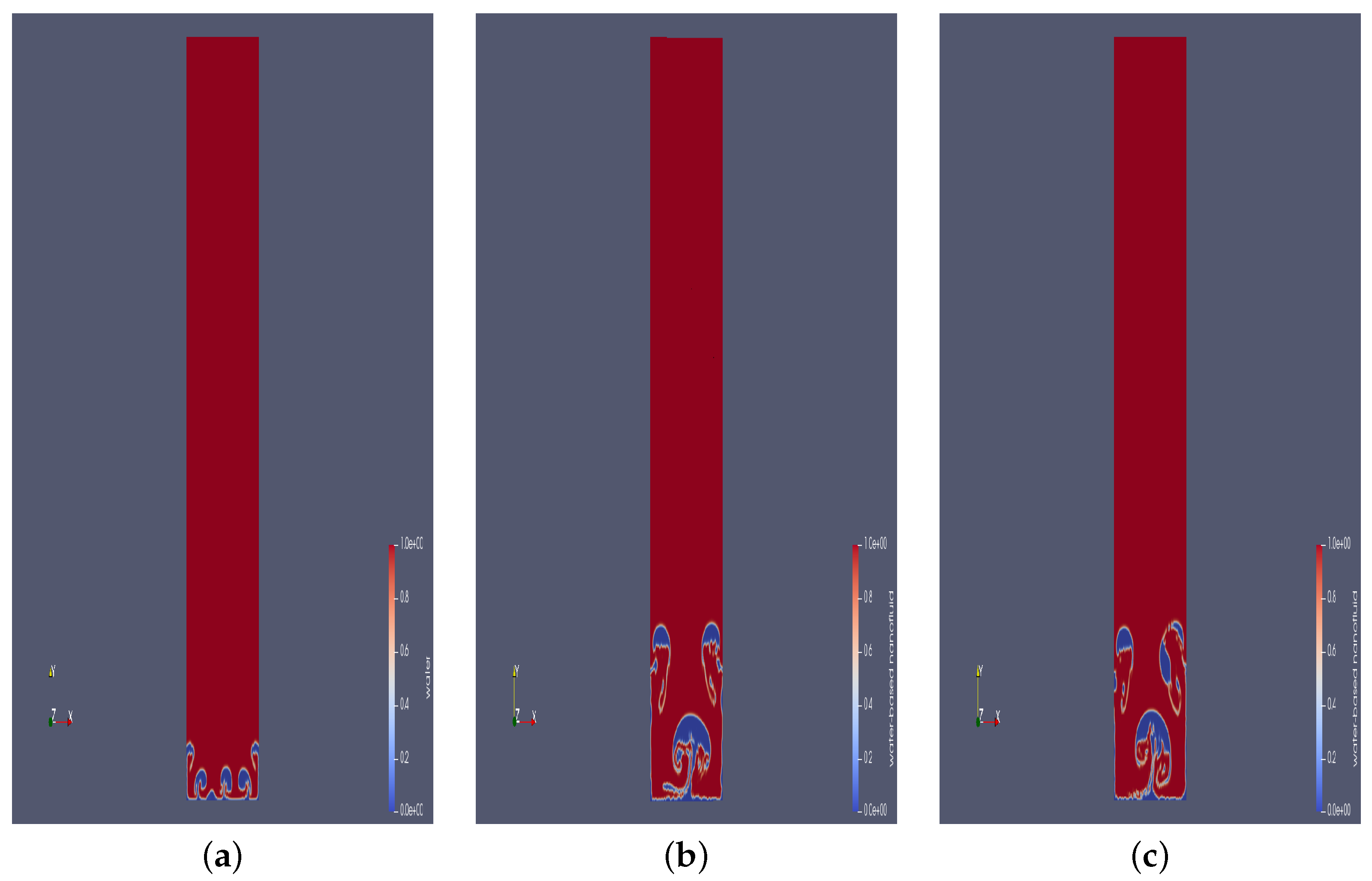
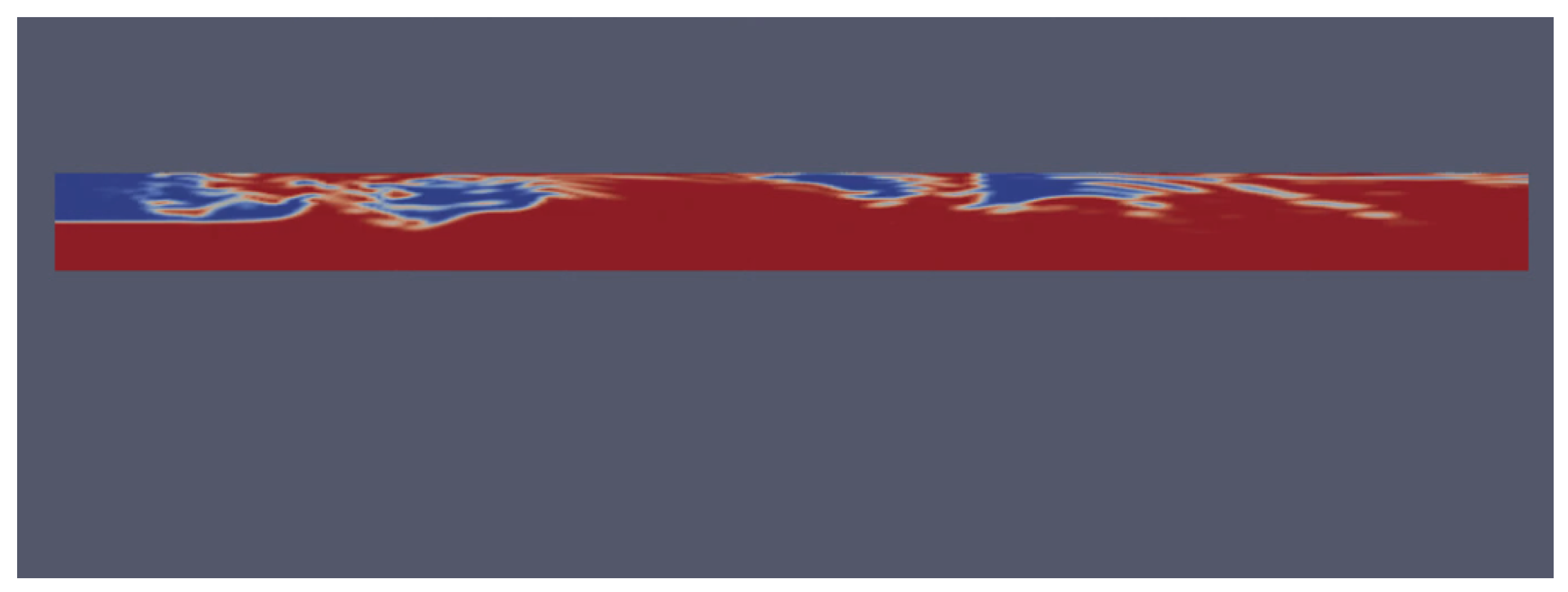
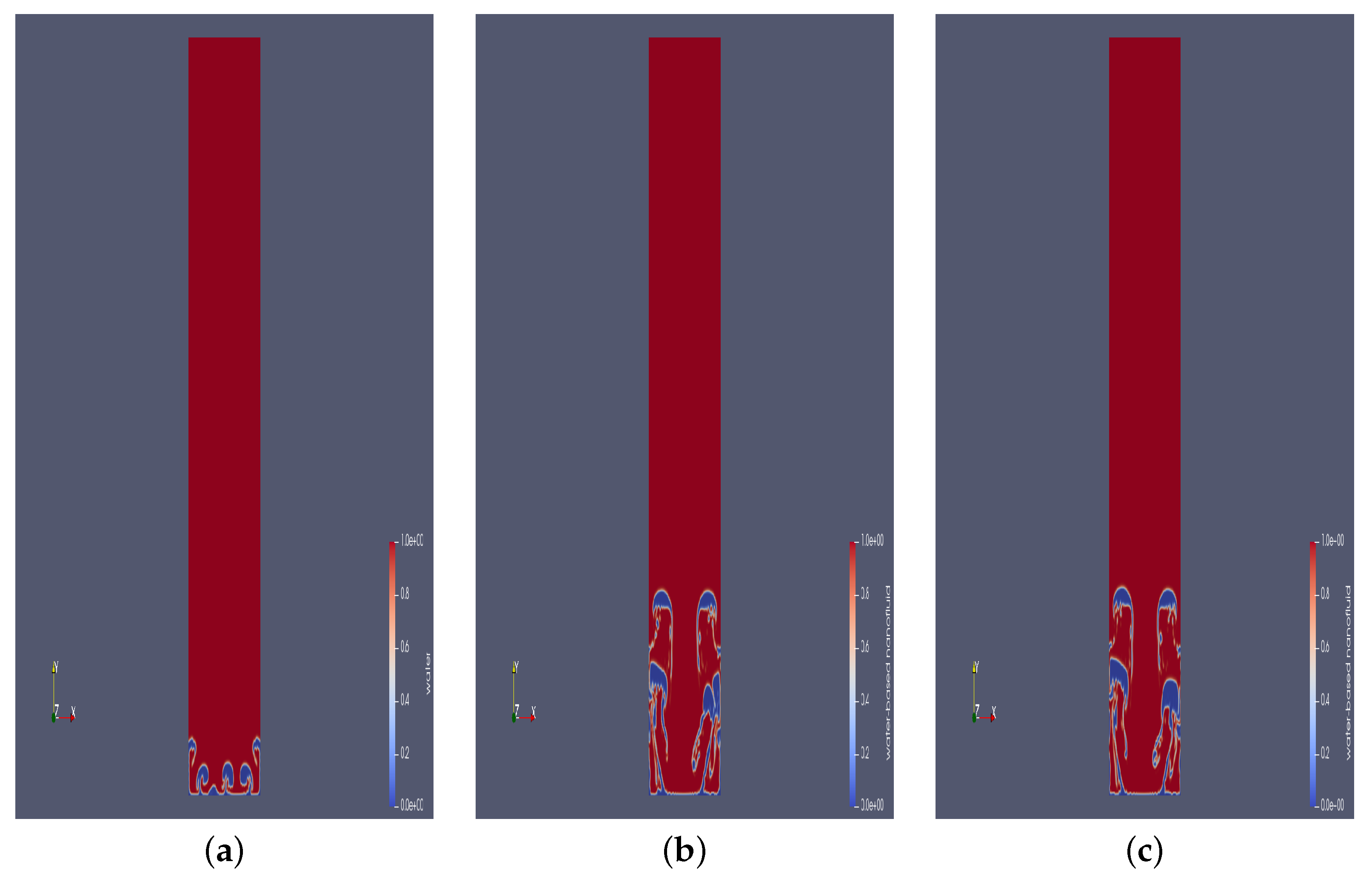
The investigation develops robust numerical algorithms for the simulation of three-phase, solid-liquid-gas, boiling flow problems in rectangular channels. The numerical algorithms are based on the finite-volume-methods (FVM) and implement both the volume-of-fluid (VOF) methods for liquid-gas interface tracking as well as the volume-fraction methods to account for the concentration of embedded solid nano-particles in the liquid phase. Water is used as the base-liquid and the solid phase is modelled via metallic nano-particles (both aluminium oxide and titanium oxide nano-particles are considered) that are homogeneously mixed within the liquid phase. The gas phase is considered as a vapour arising from the boiling processes of the liquid-phase. The finite volume methodology is implemented on the OpenFOAM software platform, specifically by careful modification and manipulation of existing OpenFOAM solvers. The computational results are presented graphically with respect to variations in time as well as in the nano-particle volume fractions. The simulations and results accurately capture the formation of vapour bubbles in the two-phase (particle-free) liquid-gas flow and additionally the computational algorithms are similarly demonstrated to accurately illustrate and capture simulated boiling processes. The presence of the nano-particles is demonstrated to enhance the heat-transfer, boiling, and bubble formation processes. The investigation lays the important groundwork to develop computational algorithms for the simulation of heat-transfer problems in coupled geometries, such as heat-exchangers, and under conditions of phase-change, boiling, condensation, variable nano-particle concentration, etc.