
Intelligent Action Planning for Well Construction Operations Demonstrated for Hole Cleaning Optimization and Automation


Abstract
1. Introduction
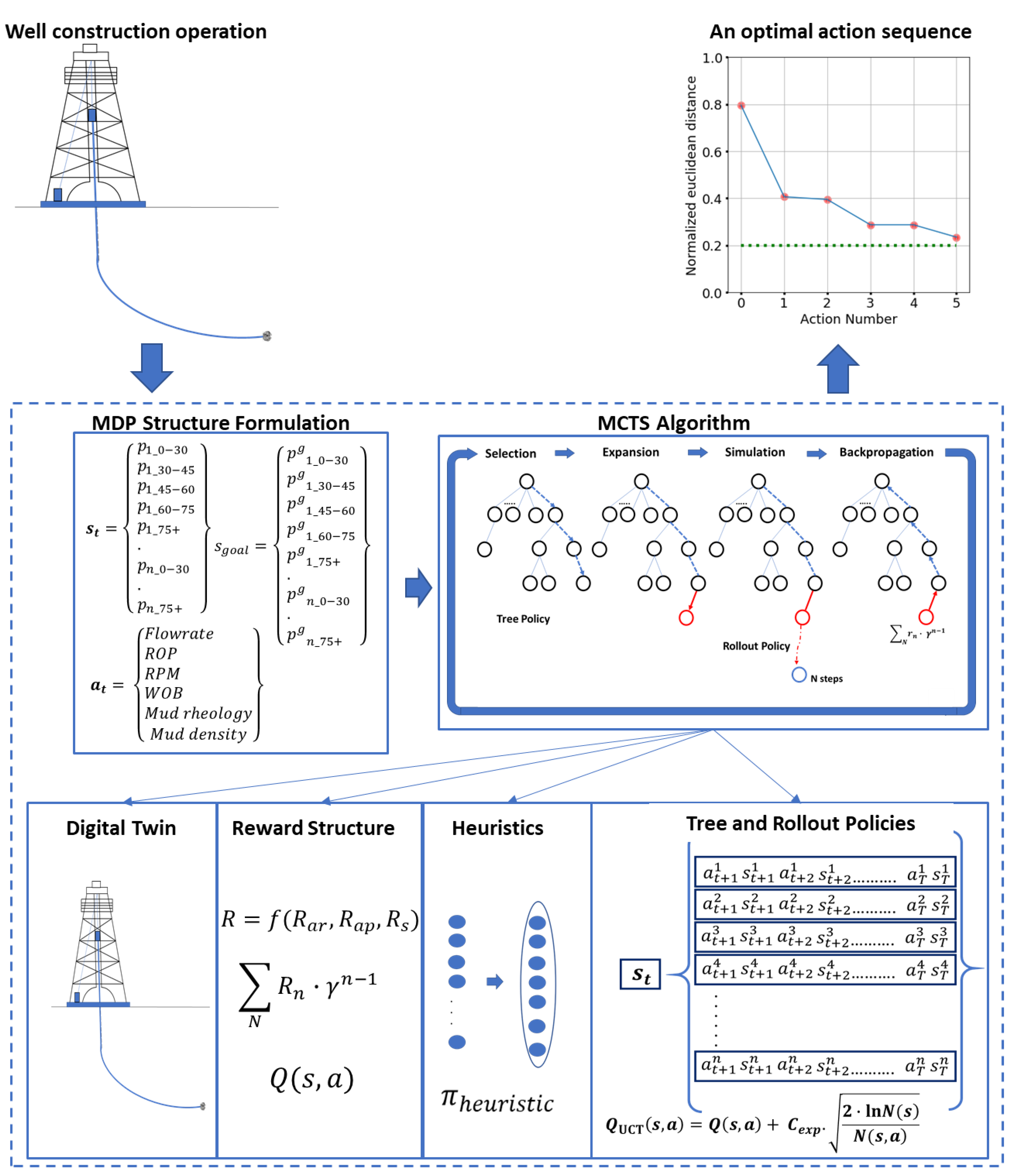
2. Setting Up Decision-Engines for Well Construction Operations
2.1. Comparison of Planning Algorithms
2.2. Utilizing SBS for Well Construction Action Planning
2.2.1. Monte Carlo Tree Search (MCTS) Algorithm
- Selection from nodes already in the search tree using the tree policy;
- Expansion of the tree at the leaf node by adding one (or more) node(s);
- Simulation or rollout of actions, using the rollout policy, until the terminal condition is met (either reaching a terminal state or the end of the planning time horizon, T);
- Backpropagation or backing the rewards up the expanded tree to update the values of different state-action pairs (Q(s, a)) encountered during the episode.
2.2.2. Structuring Well Construction Operations as Sequential Decision-Making Systems
- Identification of appropriate parameters to quantify the state () of the system, and defining the desired or goal states () based on the operation’s objective;
- Identification of relevant control variables or actions () that can affect the system state;
- Building the state-space () and the action-space () such that and for all and ;
- Incorporating problem-specific heuristics () to identify legitimate and promising actions from every state;
- Building models (digital twins) of the underlying processes to simulate the state transitions () brought about by different actions;
- Defining a method to quantify the various state action transitions, for instance, by using reward functions () to calculate long-term value functions ();
- Selection of a suitable action-planning technique to formulate a plan (—the suggested sequence of actions for successive decision epochs).
3. Design of a Planning System for Hole Cleaning Action Planning using MCTS
3.1. Setting Up the MDP
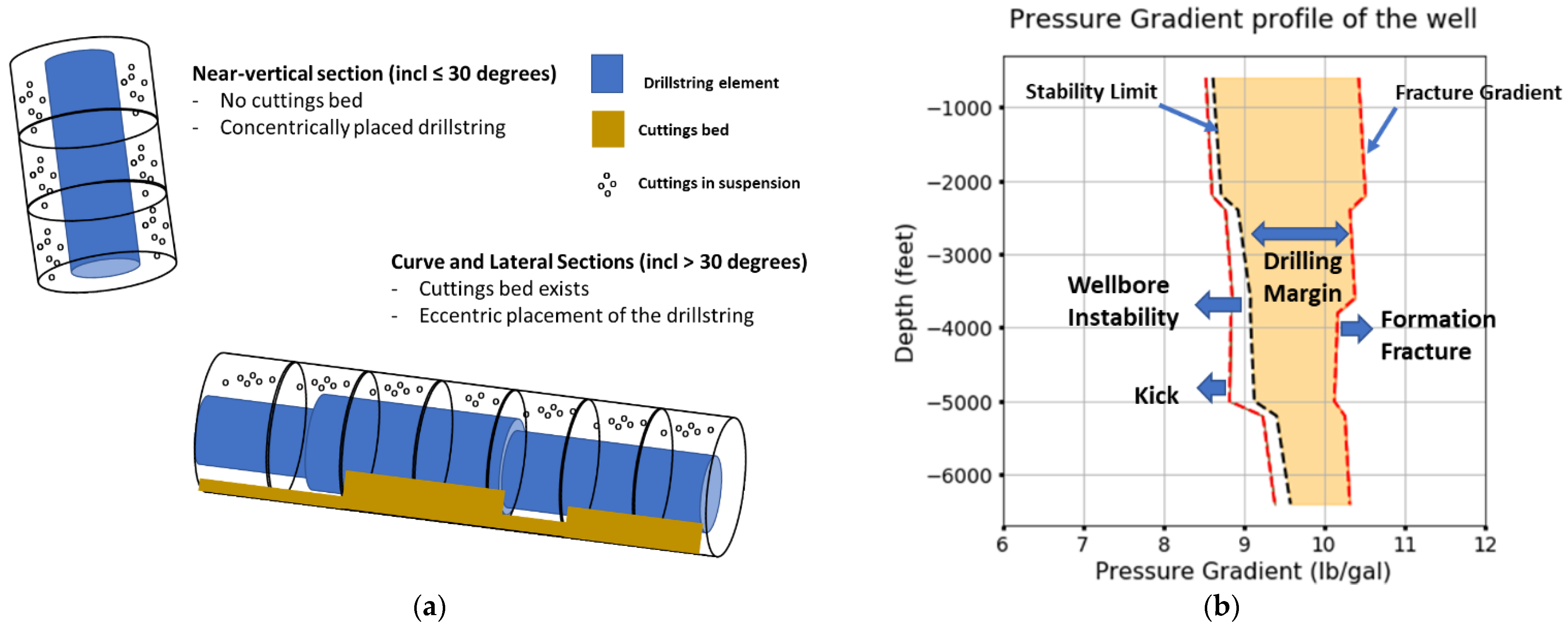
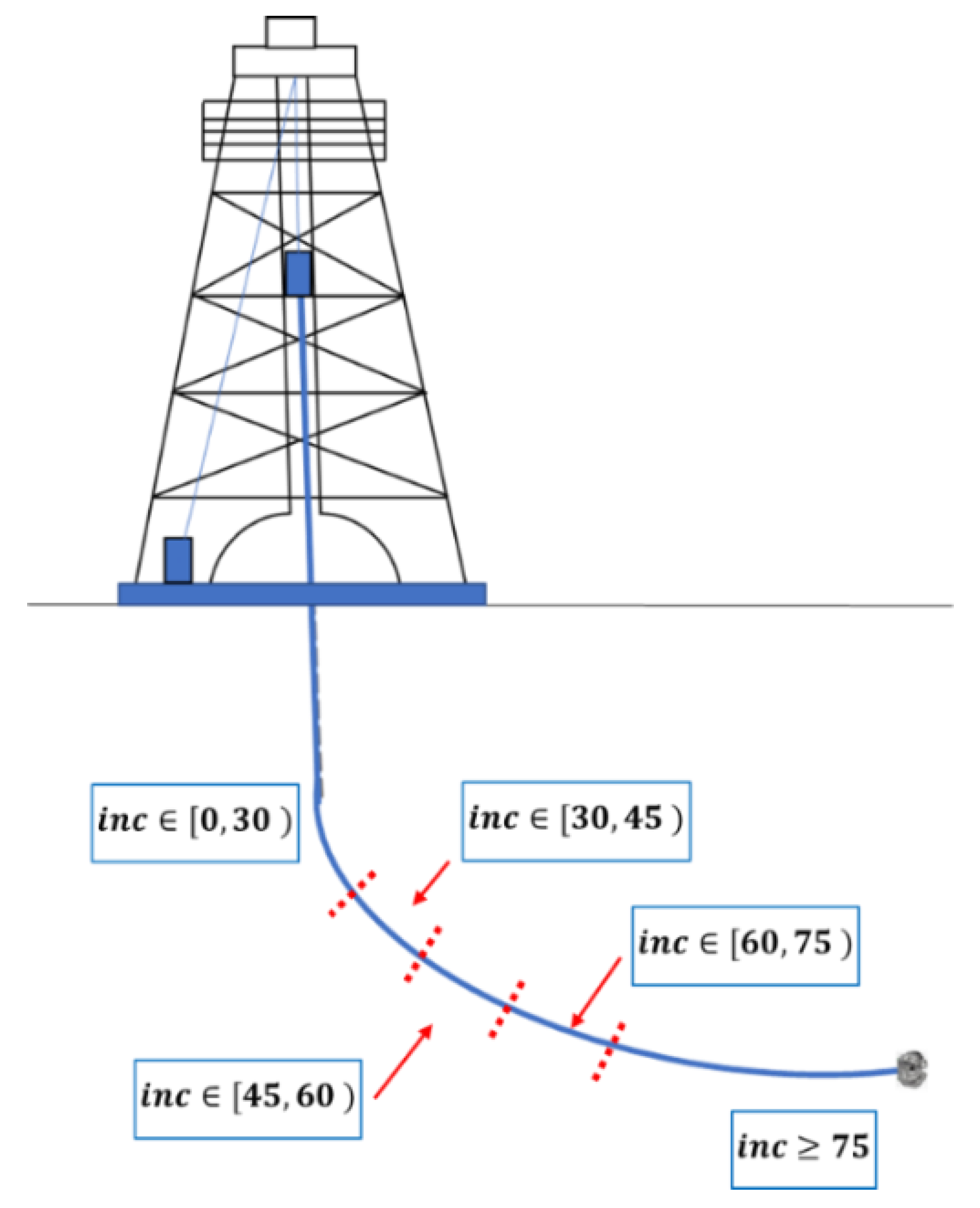
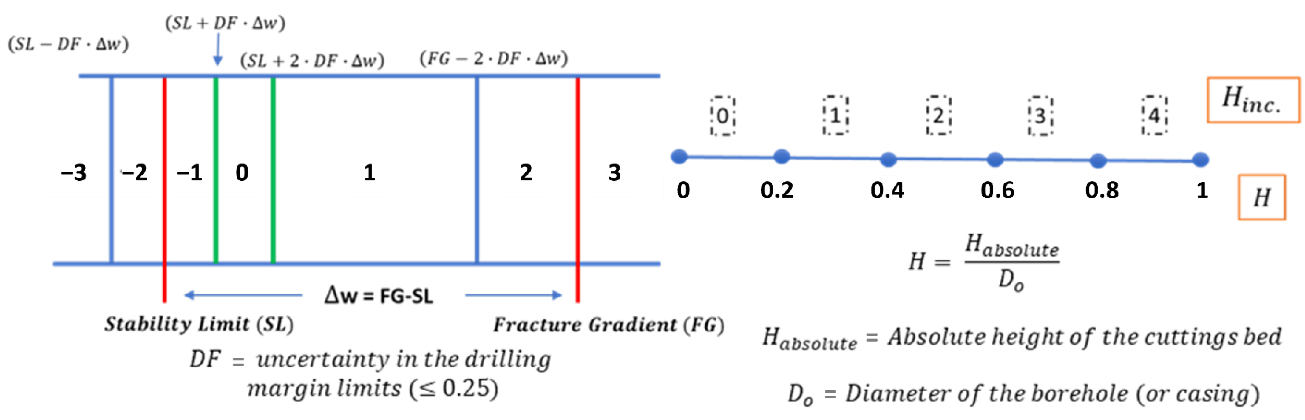
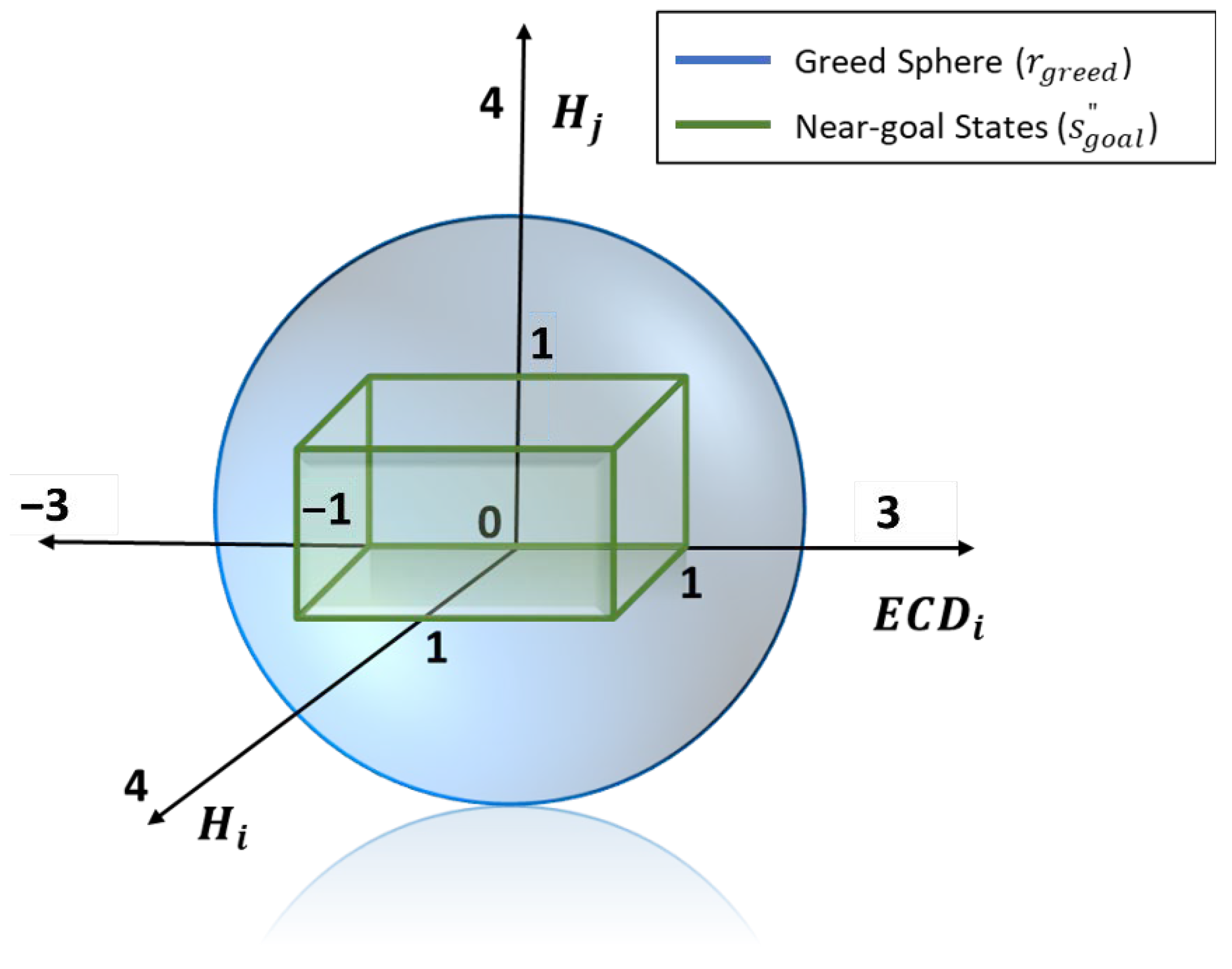
3.1.1. State-Space and the Goal State
- Height of the cuttings bed in the curve and the lateral sections of the well;
- ECD along the length of the well.
3.1.2. Action-Space
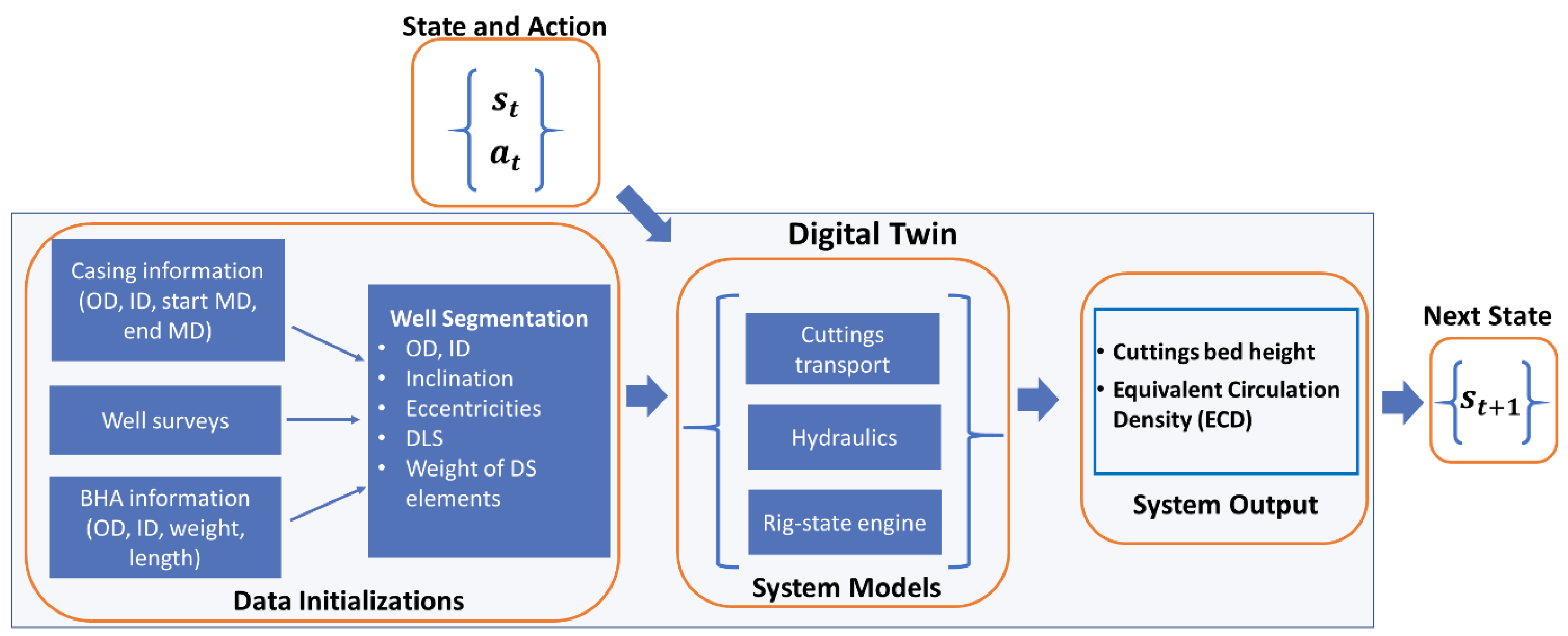
3.1.3. Digital Twin
3.1.4. Reward Function
- the reward set associated with state transition (Rs);
- the penalty set associated with action transition (Rap);
- the reward set associated with action values (Rar).
3.2. MCTS Setup for Hole Cleaning
- The agent is rewarded only when a terminal or a goal state is reached, i.e., sparse rewarding;
- From any state within the tree, all actions in its action-space (As) are evaluated by the UCT policy regardless of their practicability for the operation;
- The rollout policy is random uniform, i.e., all actions (irrespective of their feasibility) have an equal probability of being selected.
- Definition of a non-sparse reward function, such that the reward for every state-action transition during the rollout step is utilized for updating all tree nodes’ Q values. This is addressed by the reward function shaping strategy, which was discussed in the previous section;
- Using a heuristic function to improve the tree policy;
- Using a heuristic function to reduce the randomness in the rollout policy.
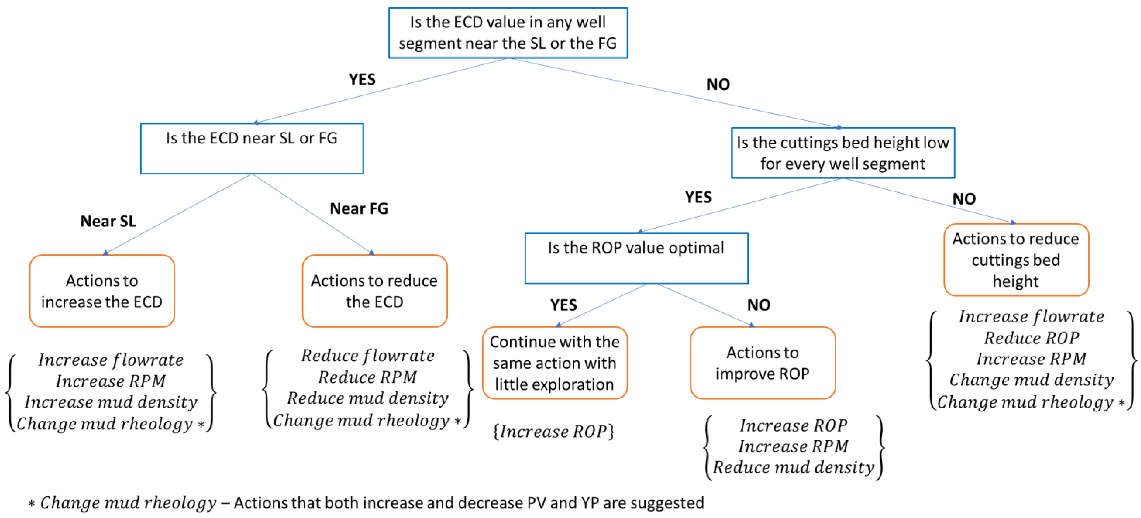
3.2.1. Heuristic Function Development
- Safety and performance metric (Asp), to prevent well control issues (such as kicks and lost circulation events) from occurring, as well as to ensure efficient cuttings bed removal and ROP maximization for optimal drilling performance;
- Performance metric, to ensure efficient cuttings bed removal and ROP maximization for optimal drilling performance;
- Sequential metric (Asq), to ensure smoother or sequential changes in values of action control variables;
- Feasibility constraints (Afe), to suggest realistic changes in values of the action control variables;
- Proximity metric (Apx), to prioritize actions based on Euclidean distance to the goal state.
3.2.2. MCTS Structure
- The current system state (st);
- The most recent action (at−1);
- The action space of the node ();
- The total number of visits to the node so far ();
- All implemented actions and the resulting transitions, i.e., all child nodes ({ai:nodei});
- The total value associated with all iterations passing through the current state (∑children i Q(st, ai));
- The parent node (nodet−1);
4. Application of the System
- well trajectory, represented by directional surveys (inclination and azimuth versus the hole depth);
- well profile, represented by the BHA, casing and bit details;
- one-second surface sensor data, for directly and indirectly measuring the drilling parameters;
- mud-checks, to determine mud density and rheology among other drilling mud properties.
4.1. Well Profile
4.2. Performance Tracking and Action Planning
4.2.1. Performance Tracking
4.2.2. Action Planning
- The final system state;
- The average return value of the action sequence (V), which is the mean of total accumulated reward over the given trajectory that results from following the action sequence.
4.2.3. Plan 1
4.2.4. Plan 2
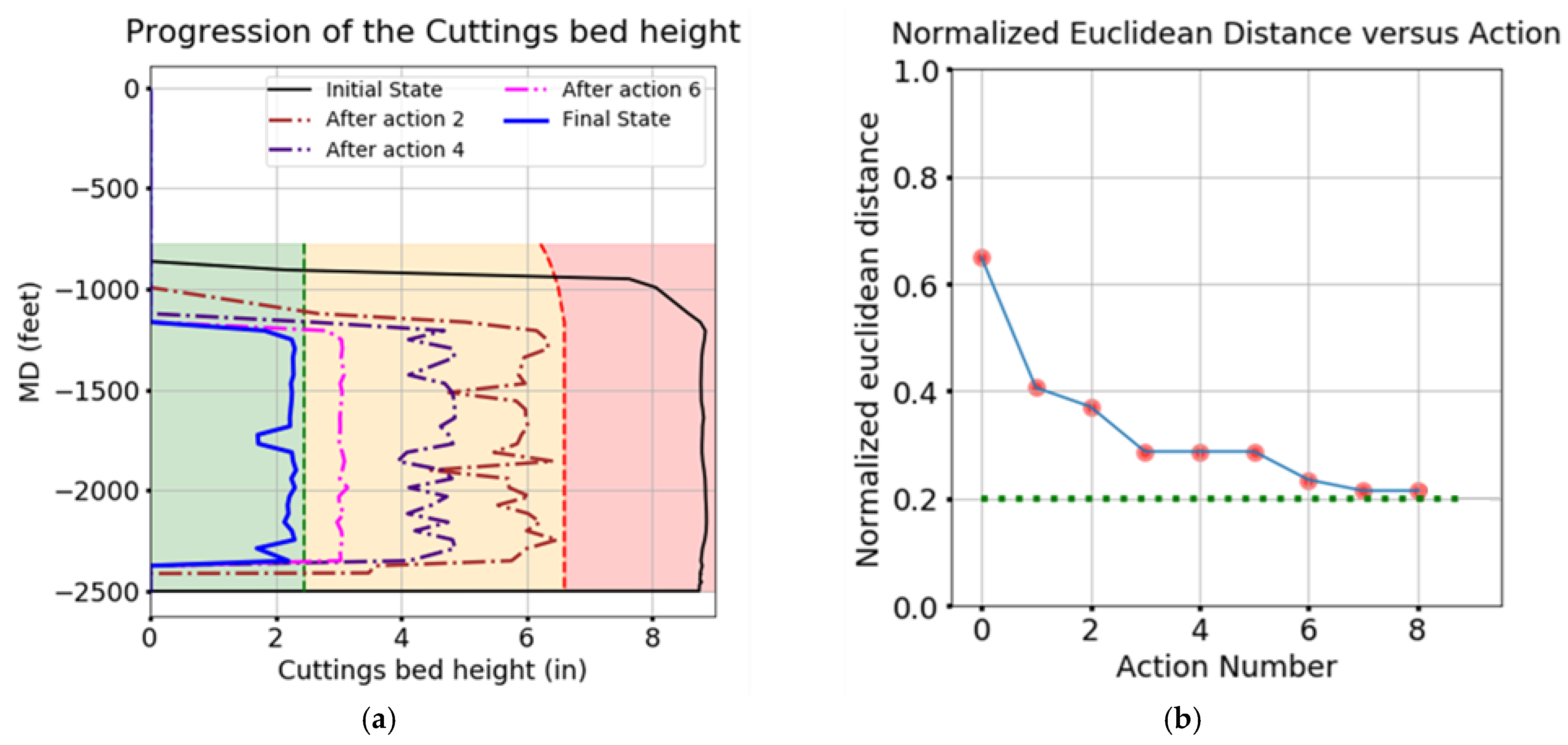
4.3. Discussion
- 1.
- The non-holonomic nature of drilling operations combined with the decision-engine’s long-term planning capabilities allow for more robust planning. An example of this is the system selecting appropriate mud properties at the beginning of the circulation cycle by evaluating multiple steps into the future. Both plans that were generated result in a better outcome than the actual plan generated and implemented by a human decision-maker.
- 2.
- Tuning the weights associated with the different reward components allows for prioritizing different objectives or different sections of the well over others.
- 3.
- Utilizing the domain-knowledge enriched MCTS allows for faster and more efficient planning, and well-defined heuristic functions make such planning systems implementable in the field. Exhaustively evaluating all nodes in the search tree to the eighth level (eight decision epochs or 40-min) would require over a hundred million simulations, as well as require storing the results of each state-action transition. This would be highly computationally and memory inefficient. MCTS, on the other hand, requires a number of simulations that are many orders of magnitude lower (only a few thousand in total), and all state-action transition results do not need to be stored. For the cases discussed in this paper, the planning algorithm, without any parallel processing or multi-threading on a standard laptop using a non-streamlined Python code, was able to generate these plans in under an hour.
- 4.
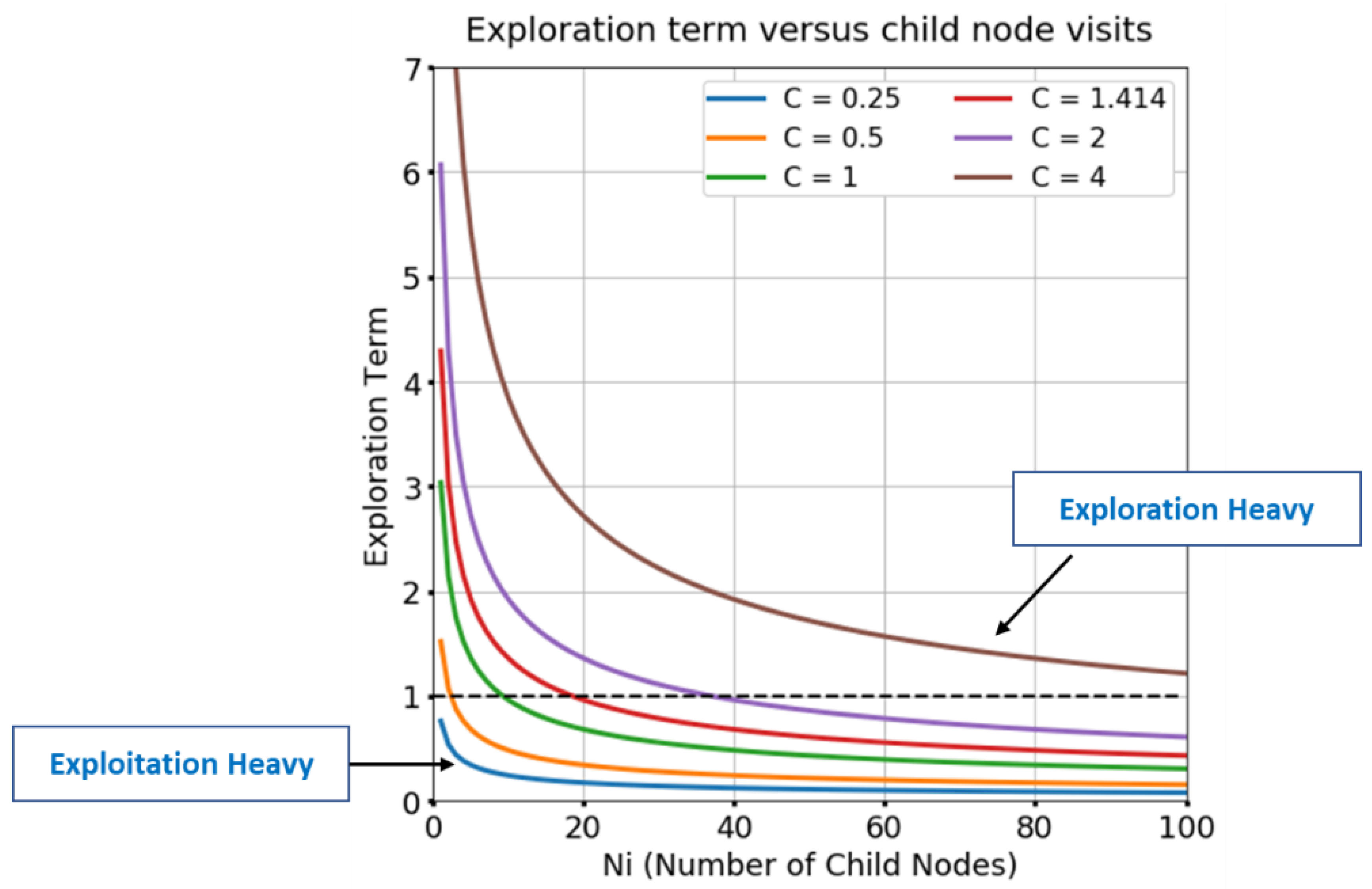
- Planning with higher values does result in the convergence of the state’s Euclidean distance towards the 0.2-line, but it requires many more simulations. On the other hand, lower Cexp values introduce an element of bias depending on the order in which the nodes are added to the tree, which itself depends on the random rollout policy for MC simulations.
5. Conclusions
- 1.
- MCTS planning systems allow for a hybrid approach to managing conflicting objectives by combining the advantages of the exploration-exploitation trade-off offered by the MCTS, with domain-knowledge derived heuristics, thereby helping make better decisions.
- 2.
- A combination of the digital twin and a non-sparse reward function, with backpropagation of the episodic returns, allows the system to learn from simulated experience. A non-sparse reward structure ensures that the feedback received by the agent is frequent and meaningful, thereby speeding up the policy improvement process.
- 3.
- The underlying tree and rollout policies of the MCTS algorithm can be enhanced by using well-defined process-specific heuristics. This assists in improving the convergence rate of the system towards an optimal action sequence. For the hole cleaning system, the heuristic was designed to balance safety, performance, feasibility, and proximity constraints.
- 4.
- Utilizing such systems can aid in overall performance improvement by eliminating the need to wait on decisions, as well as suggesting optimal drilling parameters for the given wellbore condition.
Author Contributions
Funding
Acknowledgments
Conflicts of Interest
Unit Conversion
| 1 meter (m) | 3.28 feet (ft) |
| 1 meter/second (m/s) | 11,811 feet/hour (ft/h) |
| 1 psi | 6894.76 Pa |
| 1 ppg | 119.83 kg/m3 |
| 1 radian | 57.2958 degrees |
| 1 ft3 | 0.02832 m3 |
| 1 GPM | 0.0000631 m3/s |
| 1 cP | 0.001 Pa·s |
| 1 lbf/100 ft2 | 0.4788 Pa |
| 1 lbs. | 0.4536 Kg |
Nomenclature
| Action-space | |
| Action set associated with feasibility constraints (for hole cleaning heuristic) | |
| Action set associated with proximity metric (for hole cleaning heuristic) | |
| Reduced action space for a state during the rollout phase of the MCTS | |
| Action space from state | |
| The action space of the node associated with state | |
| Action set associated with safety and performance metrics (for hole cleaning heuristic) | |
| Action set associated with sequential metric (for hole cleaning heuristic) | |
| The most recently executed action | |
| Aggressive actions representing greater magnitude changes in values of action control variables relative to the most recent action | |
| Regular actions representing small changes in action control variables with respect to the most recent action | |
| action sequence recommended by the system for the first planning case | |
| action sequence recommended by the system for the second planning case | |
| Action executed by the agent at time or decision epoch | |
| The exploration factor in the UCT formula | |
| True vertical depth for the measured depth | |
| Normalized Euclidean distance for the current state | |
| Equivalent circulation density (pounds per gallon or ppg) | |
| Functional value of ECD in the inclination interval segment | |
| The level at is in the tree | |
| Rate of flow of the drilling mud through the drillstring controlled by a positive displacement reciprocating mud pump on the surface (GPM) | |
| the net discounted return to decision epochs | |
| Acceleration due to gravity (9.81 m/s2) | |
| Functional value of the cuttings bed height in the inclination interval segment | |
| Inclination angle range (degrees) | |
| Total number of visits to the state | |
| Number of times action has been taken from state | |
| Total number of visits to the node associated with state | |
| Root node corresponding to the starting state | |
| Randomly expanded node from the leaf node during the expansion phase of the MCTS | |
| Leaf node reached at the end of the selection phase of the MCTS | |
| Node at decision epoch | |
| Frictional pressure drop in the annulus (Pa) at a measured depth | |
| Hydrostatic Pressure (Pa) at a vertical depth of | |
| Transition probability of a system in the state to the state when an agent executes action | |
| Plastic viscosity (cP) | |
| Average value associated with implementing action from state | |
| The upper confidence bound or the urgency term in the UCT formula | |
| Reward set | |
| Action reward component associated with the density value | |
| Action reward component associated with the flowrate value | |
| Action reward component associated with the PV value | |
| Action reward component associated with the ROP value | |
| Action reward component associated with the RPM value | |
| Action reward component associated with the YP value | |
| Action transition-based penalty set | |
| Normalized action penalty for the hole cleaning system | |
| Action value-based reward set | |
| Normalized action reward for the hole cleaning system | |
| State reward component associated with ECD in the inclination interval | |
| Action Penalty component associated with changing mud density | |
| Action Penalty component associated with changing flowrate | |
| State reward component associated with cuttings bed height in the inclination interval | |
| Net normalized reward function for the hole cleaning system | |
| Action Penalty component associated with changing mud PV | |
| Action Penalty component associated with changing ROP | |
| Action Penalty component associated with changing RPM | |
| State transition-based reward set | |
| Normalized state reward for the hole cleaning system | |
| Action Penalty component associated with changing mud YP | |
| Rate of penetration or drilling rate (ft/h) | |
| Drillstring rotation speed (revs./min) | |
| Radius of the greed sphere for evaluation | |
| Reward associated with the state-action transition | |
| State-space | |
| Stability limit (ppg) | |
| State of the hole cleaning system at the well TD | |
| State of the wellbore after performing a circulation cycle at TD | |
| State of the wellbore after performing a circulation cycle at TD following | |
| State of the wellbore after performing a circulation cycle at TD following | |
| Goal or desired state for the MDP | |
| The states near the goal state (for evaluating the set) | |
| State of the system at time or decision epoch | |
| Number of decision epochs to evaluate till in the future | |
| Time step or decision epoch | |
| Time available for MCTS algorithm to plan | |
| The average return value of an action sequence | |
| Weight set associated with the action transition penalty | |
| Weight value associated with the normalized action penalty | |
| Weight set associated with the action value reward | |
| Weight value associated with the normalized action reward | |
| Weight set associated with state transition reward | |
| Weight value associated with the normalized state reward | |
| Weight on bit (klbs.) | |
| Yield point (l bf/100 ft2) | |
| Policy or plan | |
| Problem specific heuristic (probability of selecting action ) | |
| Tree policy—the action selected from a given node in the search tree during the selection phase of the MCTS | |
| Discount factor for return calculation |
References
- Sadlier, A.; Says, I.; Hanson, R. Automated Decision Support to Enhance While-Drilling Decision Making: Where Does it fit Within Drilling Automation? In Proceedings of the SPE/IADC Drilling Conference, Amsterdam, The Netherlands, 5–7 March 2013. [Google Scholar] [CrossRef]
- Shokouhi, S.V.; Skalle, P. Enhancing decision making in critical drilling operations. In Proceedings of the SPE Middle East Oil and Gas Show and Conference, Manama, Bahrain, 15–18 March 2009; pp. 809–816. [Google Scholar] [CrossRef]
- Mayani, M.G.; Baybolov, T.; Rommetveit, R.; Ødegaard, S.I.; Koryabkin, V.; Lakhtionov, S. Optimizing drilling wells and increasing the operation efficiency using digital twin technology. In Proceedings of the IADC/SPE International Drilling Conference and Exhibition, Galveston, TX, USA, 3–5 March 2020. [Google Scholar] [CrossRef]
- Nadhan, D.; Mayani, M.G.; Rommetveit, R. Drilling with digital twins. In Proceedings of the IADC/SPE Asia Pacific Drilling Technology Conference and Exhibition, Bangkok, Thailand, 27–29 August 2018. [Google Scholar] [CrossRef]
- Saini, G.S.; Ashok, P.; van Oort, E.; Isbell, M.R. Accelerating well construction using a digital twin demonstrated on unconventional well data in North America. In Proceedings of the Unconventional Resources Technology Conference, Houston, TX, USA, 23–25 July 2018. [Google Scholar] [CrossRef]
- Danner, G.E. Using knowledge graphs to enhance drilling operations. In Proceedings of the Offshore Technology Conference, Houston, TX, USA, 4–7 May 2020. [Google Scholar] [CrossRef]
- Miller, P.; Gouveia, J. Applying decision trees to improve decision quality in unconventional resource development. In Proceedings of the SPE Annual Technical Conference and Exhibition, Calgary, AB, Canada, 30 September–2 October 2019. [Google Scholar] [CrossRef]
- Cordoso, J.V.; Maidla, E.E.; Idagawa, L.S. Problem detection during tripping operations in horizontal and directional wells. SPE Drill. Complet. 1995, 10, 77–83. [Google Scholar] [CrossRef]
- Zhang, F.; Miska, S.; Yu, M.; Ozbayoglu, E.; Takach, N.; Osgouei, R.E. Is Well Clean Enough? A Fast Approach to Estimate Hole Cleaning for Directional Drilling. In Proceedings of the SPE/ICoTA Coiled Tubing & Well Intervention Conference & Exhibition, The Woodlands, TX, USA, 24–25 March 2015. [Google Scholar] [CrossRef]
- Abbas, A.K.; Almubarak, H.; Abbas, H.; Dawood, J. Application of machine learning approach for intelligent prediction of pipe sticking. In Proceedings of the Society of Petroleum Engineers—Abu Dhabi International Petroleum Exhibition and Conference 2019 (ADIP 2019), Abu Dhabi, UAE, 11–14 November 2019. [Google Scholar] [CrossRef]
- Da Cruz Mazzi, V.A.; Dumlao, V.C.Q.; Mourthé, A.C.L.; Elshahawi, H.; Kim, I.; Lumens, P. Machine Learning-Enabled Digital Decision Assistant for Remote Operations. In Proceedings of the Offshore Technology Conference, Houston, TX, USA, 4–7 May 2020. [Google Scholar] [CrossRef]
- Fjellheim, R. Smart collaboration for decision making in drilling. In Proceedings of the SPE Middle East Intelligent Energy Conference and Exhibition, Manama, Bahrain, 28–30 October 2013. [Google Scholar] [CrossRef]
- Saini, G.S.; Chan, H.C.; Ashok, P.; van Oort, E.; Behounek, M.; Thetford, T.; Shahri, M. Spider bots: Database enhancing and indexing scripts to efficiently convert raw well data into valuable knowledge. In Proceedings of the Unconventional Resources Technology Conference, Houston, TX, USA, 23–25 July 2018. [Google Scholar] [CrossRef]
- Chan, H.C.; Lee, M.M.; Saini, G.S.; Pryor, M.; van Oort, E. Development and Validation of a Scenario-Based Drilling Simulator for Training and Evaluating Human Factors. IEEE Trans. Hum.-Mach. Syst. 2020, 50, 327–336. [Google Scholar] [CrossRef]
- Ji, Y.; Wang, J.; Xu, J.; Fang, X.; Zhang, H. Real-Time Energy Management of a Microgrid Using Deep Reinforcement Learning. Energies 2019, 12, 2291. [Google Scholar] [CrossRef]
- Kuznetsova, E.; Li, Y.F.; Ruiz, C.; Zio, E.; Ault, G.; Bell, K. Reinforcement learning for microgrid energy management. Energy 2013, 59, 133–146. [Google Scholar] [CrossRef]
- Guan, J.; Tang, H.; Wang, K.; Yao, J.; Yang, S. A parallel multi-scenario learning method for near-real-time power dispatch optimization. Energy 2020, 202, 117708. [Google Scholar] [CrossRef]
- Jasmin, E.A.; Imthias Ahamed, T.P.; Jagathy Raj, V.P. Reinforcement Learning approaches to Economic Dispatch problem. Int. J. Electr. Power Energy Syst. 2011, 33, 836–845. [Google Scholar] [CrossRef]
- Qi, X.; Luo, Y.; Wu, G.; Boriboonsomsin, K.; Barth, M. Deep reinforcement learning enabled self-learning control for energy efficient driving. Transp. Res. Part C Emerg. Technol. 2019, 99, 67–81. [Google Scholar] [CrossRef]
- Vandael, S.; Claessens, B.; Ernst, D.; Holvoet, T.; Deconinck, G. Reinforcement Learning of Heuristic EV Fleet Charging in a Day-Ahead Electricity Market. IEEE Trans. Smart Grid 2015, 6, 1795–1805. [Google Scholar] [CrossRef]
- Kang, D.-J.; Park, J.H.; Yeo, S.-S. Intelligent Decision-Making System with Green Pervasive Computing for Renewable Energy Business in Electricity Markets on Smart Grid. EURASIP J. Wirel. Commun. Netw. 2009, 2009, 247483. [Google Scholar] [CrossRef]
- Arulkumaran, K.; Cully, A.; Togelius, J. AlphaStar: An Evolutionary Computation Perspective. In Proceedings of the Genetic and Evolutionary Computation Conference Companion, Prague, Czech Republic, 13–17 July 2019; pp. 314–315. [Google Scholar] [CrossRef]
- Moerland, T.M.; Broekens, J.; Plaat, A.; Jonker, C.M. A0C: Alpha Zero in Continuous Action Space. arXiv 2018, arXiv:1805.09613. [Google Scholar]
- Ontanon, S.; Synnaeve, G.; Uriarte, A.; Richoux, F.; Churchill, D.; Preuss, M. A survey of real-time strategy game AI research and competition in starcraft. IEEE Trans. Comput. Intell. AI Games 2013, 5, 293–311. [Google Scholar] [CrossRef]
- Silver, D.; Sutton, R.S.; Müller, M. Temporal-difference search in computer Go. Mach. Learn. 2012, 87, 183–219. [Google Scholar] [CrossRef]
- Silver, D.; Schrittwieser, J.; Simonyan, K.; Antonoglou, I.; Huang, A.; Guez, A.; Hubert, T.; Baker, L.; Lai, M.; Bolton, A.; et al. Mastering the game of Go without human knowledge. Nature 2017, 550, 354–359. [Google Scholar] [CrossRef] [PubMed]
- Silver, D.; Hubert, T.; Schrittwieser, J.; Antonoglou, I.; Lai, M.; Guez, A.; Lanctot, M.; Sifre, L.; Kumaran, D.; Graepel, T.; et al. A general reinforcement learning algorithm that masters chess, shogi, and Go through self-play. Science 2018, 362, 1140–1144. [Google Scholar] [CrossRef] [PubMed]
- Ahmed, O.S.; Aman, B.M.; Zahrani, M.A.; Ajikobi, F.I.; Aramco, S. Stuck Pipe Early Warning System Utilizing Moving Window Machine Learning Approach. In Proceedings of the Abu Dhabi International Petroleum Exhibition & Conference, Abu Dhabi, UAE, 11–14 November 2019. [Google Scholar]
- Forshaw, M.; Becker, G.; Jena, S.; Linke, C.; Hummes, O. Automated hole cleaning monitoring: A modern holistic approach for NPT reduction. In Proceedings of the International Petroleum Technology Conference, Dhahran, Saudi Arabia, 13–15 January 2020. [Google Scholar] [CrossRef]
- LaValle, S.M. Planning Algorithms; Cambridge University Press: Cambridge, UK, 2006. [Google Scholar] [CrossRef]
- Poole, D.L.; Mackworth, A.K. Artificial Intelligence: Foundations of Computational Agents, 2nd ed.; Cambridge University Press: Cambridge, UK, 2017. [Google Scholar]
- Bennett, B. Graphs: Breadth First Search vs. Depth First Search [WWW Document]. 2019. Available online: https://medium.com/javascript-in-plain-english/graphs-breadth-first-search-vs-depth-first-search-d9908c560642 (accessed on 1 July 2020).
- Mussmann, S.; See, A. Graph Search Algorithms. 2017. Available online: http://cs.stanford.edu/people/abisee/gs.pdf (accessed on 1 June 2020).
- Alija, A.S. Analysis of Dijkstra’s and A* Algorithm to Find the Shortest Path. Ph.D. Thesis, Universiti Tun Hussein Onn Malaysia, Batu Pahat, Malaysia, 2015. [Google Scholar]
- Reddy, H. Path Finding—Dijkstra’s and A* Algorithm’s. Int. J. IT Eng. 2013, 1–15. [Google Scholar]
- Bhaumik, D.; Khalifa, A.; Green, M.C.; Togelius, J. Tree Search vs Optimization Approaches for Map Generation. arXiv 2019, arXiv:1903.11678. [Google Scholar]
- Cui, X.; Shi, H. A*-based Pathfinding in Modern Computer Games. Int. J. Comput. Sci. Netw. Secur. 2011, 11, 125–130. [Google Scholar]
- Klein, S. Attacking SameGame using Monte-Carlo Tree Search: Using Randomness as Guidance in Puzzles. Master’s Thesis, KTH Royal Institute of Technology, Stockholm, Sweden, 2015. [Google Scholar]
- Li, L.K.; Seng, K.P.; Yeong, L.S.; Ch’ng, S.I.; Li-Minn, A. The Boundary Iterative-Deepening Depth-First Search Algorithm. Int. J. Adv. Comput. Sci. Its Appl. 2014, 4, 45–50. [Google Scholar]
- Korkmaz, M.; Durdu, A. Comparison of optimal path planning algorithms. In Proceedings of the 2018 14th International Conference on Advanced Trends in Radioelecrtronics, Telecommunications and Computer Engineering (TCSET), Slavske, Ukraine, 20–24 January 2018; pp. 255–258. [Google Scholar] [CrossRef]
- Sutton, R.S.; Barto, A.G. Reinforcement Learning: An Introduction, 2nd ed.; The MIT Press: Cambridge, MA, USA, 2018. [Google Scholar]
- Silver, D. Reinforcement Learning and Simulation-Based Search in Computer Go; University of Alberta: Alberta, AB, Canada, 2009. [Google Scholar]
- Cayeux, E.; Mihai, R.; Carlsen, L.; Stokka, S. An approach to autonomous drilling. In Proceedings of the IADC/SPE International Drilling Conference and Exhibition, Galveston, TX, USA, 3–5 March 2020. [Google Scholar] [CrossRef]
- Mitchell, R.F.; Miska, S.Z. Fundamentals of Drilling Engineering; Society of Petroleum Engineers: Richardson, TX, USA, 2011. [Google Scholar]
- James, S.; Konidaris, G.; Rosman, B. An analysis of Monte Carlo tree search. In Proceedings of the 31st AAAI Conference on Artificial Intelligence, San Francisco, CA, USA, 4–9 February 2017; pp. 3576–3582. [Google Scholar]
- Vodopivec, T.; Samothrakis, S.; Ŝter, B. On Monte Carlo Tree Search and Reinforcement Learning. J. Artif. Intell. Res. 2017, 60, 881–936. [Google Scholar] [CrossRef]
- Browne, C.B.; Powley, E.; Whitehouse, D.; Lucas, S.M.; Cowling, P.I.; Rohlfshagen, P.; Tavener, S.; Perez, D.; Samothrakis, S.; Colton, S. A Survey of Monte Carlo Tree Search Methods. IEEE Trans. Comput. Intell. AI Games 2012, 4, 1–43. [Google Scholar] [CrossRef]
- Kocsis, L.; Szepesvári, C.; Willemson, J. Improved Monte-Carlo Search; Technical. Repotrt 1; University of Tartu: Tartu, Estonia, 2006. [Google Scholar]
- Vodopivec, T. Monte Carlo Tree Search Strategies; Maastricht University: Maastricht, The Netherlands, 2018. [Google Scholar]
- Chaslot, G.; Bakkes, S.; Szitai, I.; Spronck, P. Monte-carlo tree search: A New Framework for Game AI. In Proceedings of the AAAI Conference on Artificial Intelligence and Interactive Digital Entertainment, Stanford, CA, USA, 22–24 October 2008; pp. 389–390. [Google Scholar]
- Chaslot, G.M.J.-B.; Winands, M.H.M.; van den Herik, H.J.; Uiterwijk, J.W.H.M.; Bouzy, B. Progressive Strategies for Monte-Carlo Tree Search. New Math. Nat. Comput. 2008, 4, 343–357. [Google Scholar] [CrossRef]
- Gelly, S.; Silver, D. Monte-Carlo tree search and rapid action value estimation in computer Go. Artif. Intell. 2011, 175, 1856–1875. [Google Scholar] [CrossRef]
- Efroni, Y.; Dalal, G.; Scherrer, B.; Mannor, S. How to Combine Tree-Search Methods in Reinforcement Learning. In Proceedings of the AAAI Conference on Artificial Intelligence, Honolulu, HI, USA, 27 January–1 February 2019; Volume 33, pp. 3494–3501. [Google Scholar] [CrossRef]
- Puterman, M.L. Markov Decision Processes, Wiley Series in Probability and Statistics; John Wiley & Sons, Inc.: Hoboken, NJ, USA, 1994. [Google Scholar] [CrossRef]
- Bourgoyne, A.T.; Millheim, K.K.; Chenevert, M.E.; Young, F.S. Applied Drilling Engineering; Society of Petroleum Engineers: Richardson, TX, USA, 1986. [Google Scholar]
- Ozbayoglu, M.E.; Saasen, A.; Sorgun, M.; Svanes, K. Effect of Pipe Rotation on Hole Cleaning for Water-Based Drilling Fluids in Horizontal and Deviated Wells. In Proceedings of the IADC/SPE Asia Pacific Drilling Technology Conference and Exhibition, Jakarta, Indonesia, 25–27 August 2008. [Google Scholar] [CrossRef]
- Sanchez, R.A.; Azar, J.J.; Bassal, A.A.; Martins, A.L. The Effect of Drillpipe Rotation on Hole Cleaning During Directional Well Drilling. In Proceedings of the SPE/IADC Drilling Conference, Amsterdam, The Netherlands, 4–6 March 1997. [Google Scholar] [CrossRef]
- Baldino, S.; Osgouei, R.E.; Ozbayoglu, E.; Miska, S.; Takach, N.; May, R.; Clapper, D. Cuttings settling and slip velocity evaluation in synthetic drilling fluids. In Proceedings of the Offshore Mediterranean Conference and Exhibition, Ravenna, Italy, 25–27 March 2015. [Google Scholar]
- Cayeux, E.; Mesagan, T.; Tanripada, S.; Zidan, M.; Fjelde, K.K. Real-time evaluation of hole-cleaning conditions with a transient cuttings-transport model. SPE Drill. Complet. 2014, 29, 5–21. [Google Scholar] [CrossRef]
- Gul, S.; van Oort, E.; Mullin, C.; Ladendorf, D. Automated Surface Measurements of Drilling Fluid Properties: Field Application in the Permian Basin. SPE Drill. Complet. 2020, 35, 525–534. [Google Scholar] [CrossRef]
- Nazari, T.; Hareland, G.; Azar, J.J. Review of Cuttings Transport in Directional Well Drilling: Systematic Approach. In Proceedings of the SPE Western Regional Meeting, Anaheim, CA, USA, 27–29 May 2010. [Google Scholar] [CrossRef]
- Saini, G.S.; Ashok, P.; van Oort, E. Predictive Action Planning for Hole Cleaning Optimization and Stuck Pipe Prevention Using Digital Twinning and Reinforcement Learning. In Proceedings of the IADC/SPE International Drilling Conference and Exhibition, Galveston, TX, USA, 3–5 March 2020. [Google Scholar] [CrossRef]
- De Oliveira, G.L.; Zank, C.A.C.; De Costa, A.F.S.; Mendes, H.M.; Henriques, L.F.; Mocelin, M.R.; De Oliveira Neto, J. Offshore drilling improvement through automating the rig state detection process—Implementation process history and proven success. In Proceedings of the IADC/SPE Drilling Conference and Exhibition, Fort Worth, TX, USA, 1–3 March 2016. [Google Scholar] [CrossRef]


| Inclination Interval | Stability Limit (ppg) | Fracture Gradient (ppg) |
|---|---|---|
| [0, 30)—in casing | 6 | 18 |
| [30, 45) | 8.2 | 10.6 |
| [45, 60) | 8.4 | 10.4 |
| [60, 75) | 8.2 | 10.2 |
| [75+) | 8.6 | 10.0 |
| Control Variable | Number of Discrete Values | Range of Values |
|---|---|---|
| Flowrate (GPM) | 10 | [0, 1800] |
| Drilling ROP (ft/h) | 10 | [0, 900] |
| Drillstring RPM (rev/min) | 10 | [0, 180] |
| Mud Density (ppg) | 5 | [8.5, 9.7] |
| Mud Plastic Viscosity (cP) | 5 | [7, 42] |
| Mud Yield Point (lbf/100 ft2) | 5 | [7, 42] |
| Drilling | Circulation |
| Control Variable | Number of Discrete Values | Range of Values |
|---|---|---|
| Flowrate (GPM) | 10 | [0, 1500] |
| Drillstring RPM (rev/min) | 10 | [0, 150] |
Publisher’s Note: MDPI stays neutral with regard to jurisdictional claims in published maps and institutional affiliations. |
© 2022 by the authors. Licensee MDPI, Basel, Switzerland. This article is an open access article distributed under the terms and conditions of the Creative Commons Attribution (CC BY) license (https://creativecommons.org/licenses/by/4.0/).
Share and Cite
Saini, G.S.; Pournazari, P.; Ashok, P.; van Oort, E. Intelligent Action Planning for Well Construction Operations Demonstrated for Hole Cleaning Optimization and Automation. Energies 2022, 15, 5749. https://doi.org/10.3390/en15155749
Saini GS, Pournazari P, Ashok P, van Oort E. Intelligent Action Planning for Well Construction Operations Demonstrated for Hole Cleaning Optimization and Automation. Energies. 2022; 15(15):5749. https://doi.org/10.3390/en15155749
Chicago/Turabian StyleSaini, Gurtej Singh, Parham Pournazari, Pradeepkumar Ashok, and Eric van Oort. 2022. "Intelligent Action Planning for Well Construction Operations Demonstrated for Hole Cleaning Optimization and Automation" Energies 15, no. 15: 5749. https://doi.org/10.3390/en15155749
APA StyleSaini, G. S., Pournazari, P., Ashok, P., & van Oort, E. (2022). Intelligent Action Planning for Well Construction Operations Demonstrated for Hole Cleaning Optimization and Automation. Energies, 15(15), 5749. https://doi.org/10.3390/en15155749