Development and Performance Verification of Frequency Control Algorithm and Hardware Controller Using Real-Time Cyber Physical System Simulator

Abstract

Frequency stability is a critical factor in maintaining the quality of the power grid system. A battery energy storage system (BESS) with quick response and flexibility has recently been used as a primary frequency control (PFC) resource, and many studies on its control algorithms have been conducted. The cyber physic system (CPS) simulator, which can perform virtual physical modelling and verification of many hardware systems connected to the network, is an optimal solution for the performance verification of control algorithms and hardware systems. This study introduces a large-scale real-time dynamic simulator that includes the national power system. This simulator comprises a power grid model, an energy management system (EMS) model, a BESS system model, and a communication model. It performs the control algorithm performance evaluation and the hardware controller’s response performance evaluation. The performance of the control algorithm was evaluated by tracking the power system’s characteristic trajectory in the transient state based on the physical response delay time between the output instruction of the frequency regulation controller (FRC), a hardware controller, and the output response of the BESS. Based on this, we examined the response performance evaluation results by linking them to the optimally designed actual FRC. As a result, we present an analysis of the BESS’s characteristic trajectories in the transient state, such as frequency, power system inertia, and power grid constant, and provide FRC response performance evaluation results at a level of 163 ms, by connecting the BESS installed at the actual site with the CPS simulator.

1. Introduction

Recently, power grid systems have been operated based on conventional fossil fuel-oriented centralised power plants (CPPs) and also distributed power sources of renewable energy. This is due to the global eco-friendly energy policy stance and emerging countries’ efforts to improve electrification ratio. This phenomenon has advantages such as carbon emission reduction and power generation cost reduction, but there are problems in the frequency control part due to the phenomena of the system’s complexity, intermittent power generation, and system inertia decline. Power generation increased as the proportion of distributed power source installations using renewable energy sources increased, but it also brought problems, such as a decrease in system inertia and frequency changes due to power output changes owing to intermittent outputs. A battery energy storage system (BESS) with high flexibility and fast responsiveness is gaining traction as a solution to this problem. The BESS can perform the roles of power generation and load because it can charge and discharge. Therefore, it can alleviate the power output changes of intermittent distributed power sources and can also be used in frequency controls since it responds quickly in a low-inertia system. As a result, it is widely used as a resource for primary frequency control (PFC). The main areas of research related to this can be classified into research on the development of physical models and research on optimal operation strategies for PFC. The physical model domain of the BESS is divided into dynamic models for a single battery [1,2,3], dynamic models at the battery pack level [4,5], and dynamic models at the energy storage system level [6,7,8]. Studies on physical models form the basis of development research on optimal operation strategies for PFC that reflect the properties of batteries. Based on this, simulation studies have been conducted for optimal operation strategies. The main research areas are research on the effectiveness and feasibility assessment of BESS for PFC [9,10,11,12,13,14,15], optimal SOC operation strategies of BESS for PFC [16,17], and optimal droop control and inertia control strategies of BESS for PFC [18,19,20,21,22]. As such, virtual physical models of BESS have been used in PFC simulations to analyse the characteristics of the BESS operated by PFC or the characteristics of the power system, resulting in the development of optimal operation strategies.

However, most previous studies did not consider the physical response delay time that occurs between the PFC hardware controller for the BESS and the power conditioning system (PCS). If a frequency transient state occurs in a low-inertia system, the rate of change of frequency (RoCoF) decreases rapidly in the initial stage. In this case, the inhibition of RoCoF may vary depending on how quickly the output of BESS is put in. To examine this, it is necessary to track the power system’s characteristic trajectories in a short time, considering the response delay time of the BESS and the amount of PFC response provided by the CPP. Because of this, these characteristics cannot be examined in detail when closed-loop-type simulations or power system equivalent models are used, as in the aforementioned previous studies. As a result, the concept of cyber physical system (CPS) has recently emerged, which connects many hardware systems linked by a network with virtual physical systems. In general, the target CPS is a hybrid system because it includes both analogue continuous elements (such as physical elements and electricity) and digital discrete elements (such as control algorithms). In a power grid system, therefore, analogue continuous models, such as power generation, power transmission, and load, should be implemented to construct CPS-type systems, and digital discrete models, such as control algorithms and hardware controllers, should be distinguished and developed. Furthermore, the simulation-based model verification techniques, software in the loop simulation (SILS) and hardware in the loop simulation (HILS), should be constructed to provide a basis for verifying the target model’s control algorithms and hardware controllers. As can be seen in recent research cases, the following studies have been conducted: performance verification of Volt-Var optimization engine using IEC61850t-Var [23], co-simulation verification of power and communication systems for dynamic analysis of a micro-grid [24], verification of wide-area communication platform for power grid monitoring system [25], efficiency verification of wireless communication technology in a power system [26,27], and investigation of the impacts of cyber contingency on power system operation [28]. As such, CPS simulations can implement new power operation systems and solutions in simulations to evaluate the impacts and validity of the system’s control algorithms and communication systems, which are to be adopted.

As a result, this study employs CPS simulations to obtain real-time characteristic trajectory analysis results based on the effects of the BESS response delay time for PFC, as well as to implement hierarchical multi-systems of hardware as virtual physical systems to provide results evaluating the response performance of the hardware controllers.

Section 2 introduces A1GridSim, named as advanced real-time dynamic power grid simulator for CPS developed using ProTRAX software. The concept design began development in 2014, and the first prototype and its results were published in 2016 [29]. It consists of a power grid model that includes power generation, power transmission, power transformation, and load; a BESS model that includes batteries, PCS, and FRC; and a communication model that includes the protocols of DNP3.0 and Modbus. Two types of verification and evaluation studies were conducted to test the performance and various functions of the developed simulator. Section 3 shows the results of SILS for the comparative verification of the dynamic frequency model of A1GridSim based on the transient state frequency history data; characteristic trajectory analysis in the transient state of the BESS for PFC; and the impact of the BESS and the characteristic trajectory analysis of the power system according to the physical response delay time (PRDT) between the PCS and FRC. Section 4 constructs the hierarchical multi-system of the actual hardware system and performs co-simulation with the hardware controller installed on-site to show the results of HILS for the performance evaluation.

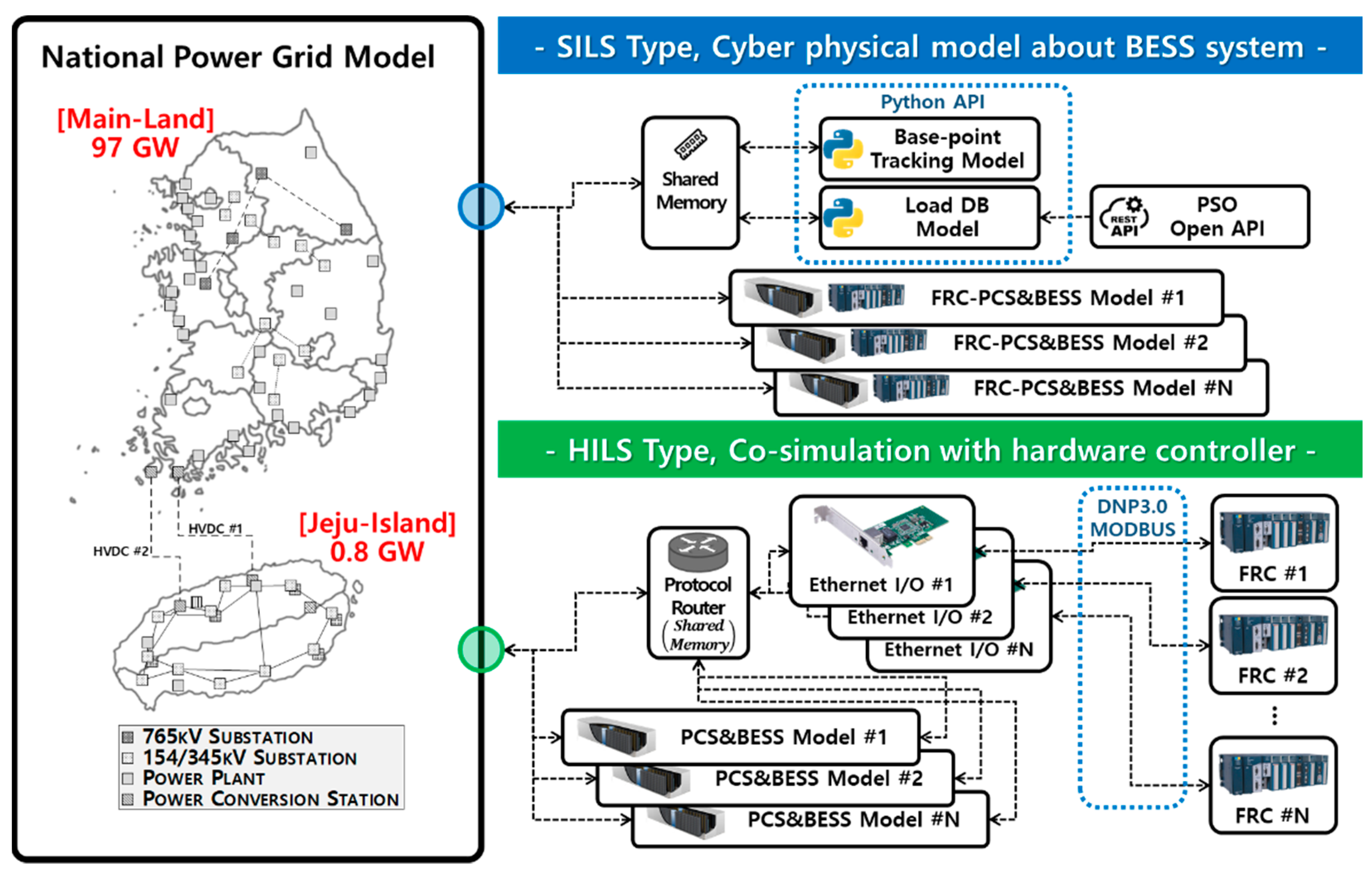
2. Development of Co-Simulation “A1GridSim”

The name of the CPS simulator developed in this study is “A1GridSim”, and it was developed using the ProTRAX software, which provides a real-time dynamic simulation environment [30]. ProTRAX provides high-quality, high-fidelity virtual physical components, such as a boiler, combine cycle, circulating fluidized bed (CFB), the balance of plant, AC/DC electric power, and renewable energy. It is used as simulation software for CPS and digital-twins by providing programmable malfunctions that can simulate the transient state of each physical component; an emulator function for a distributed control system; and an application programming interface (API) function for the linkage with external solvers.

As shown in Figure 1, “A1GridSim” shows the configuration of the national power system, targeting the power system of South Korea. The national power grid model connects the mainland power grid of 97 GW and the Jeju island power grid of 0.8 GW with a total of four HVDC lines. The main components consist of 177 CPPs and power transmission and transformation facilities of the 154, 345, and 765 kV classes.

The simulation mode can be selectable into the SILS or HILS type. The SILS type is used to analyse PFC operation algorithms by modelling the BESS for PFC as a virtual physical model. In addition, the HILS type is used to evaluate the performance of hardware equipment by building batteries and PCS as virtual physical systems among hierarchical multi-systems and configuring a communication model that can link up with the actual FRC using DNP3.0 and Modbus protocols. As a result, this section introduces the main components of A1GridSim, which are a CPP model, an EMS model, a dynamic frequency model, and a BESS system model.

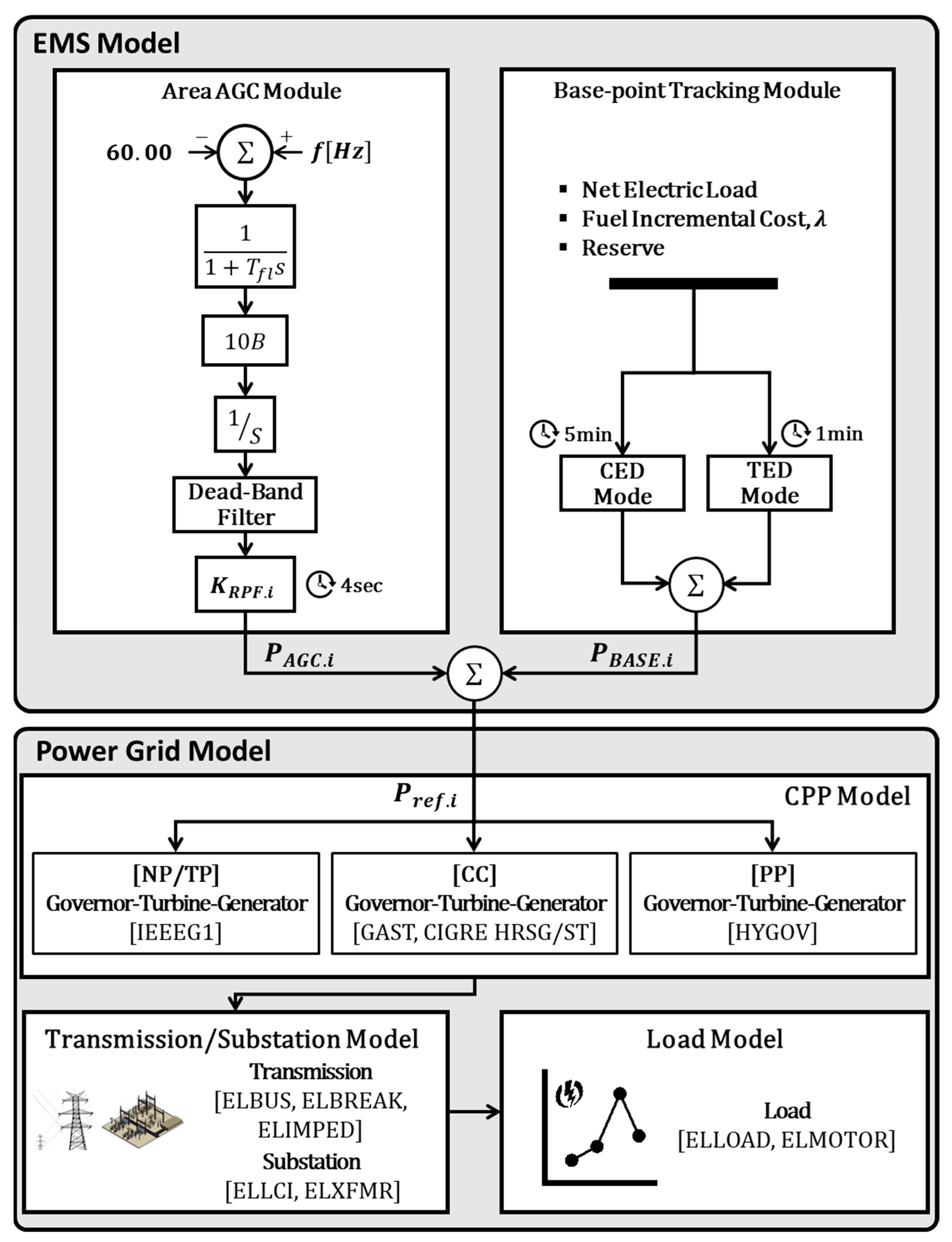
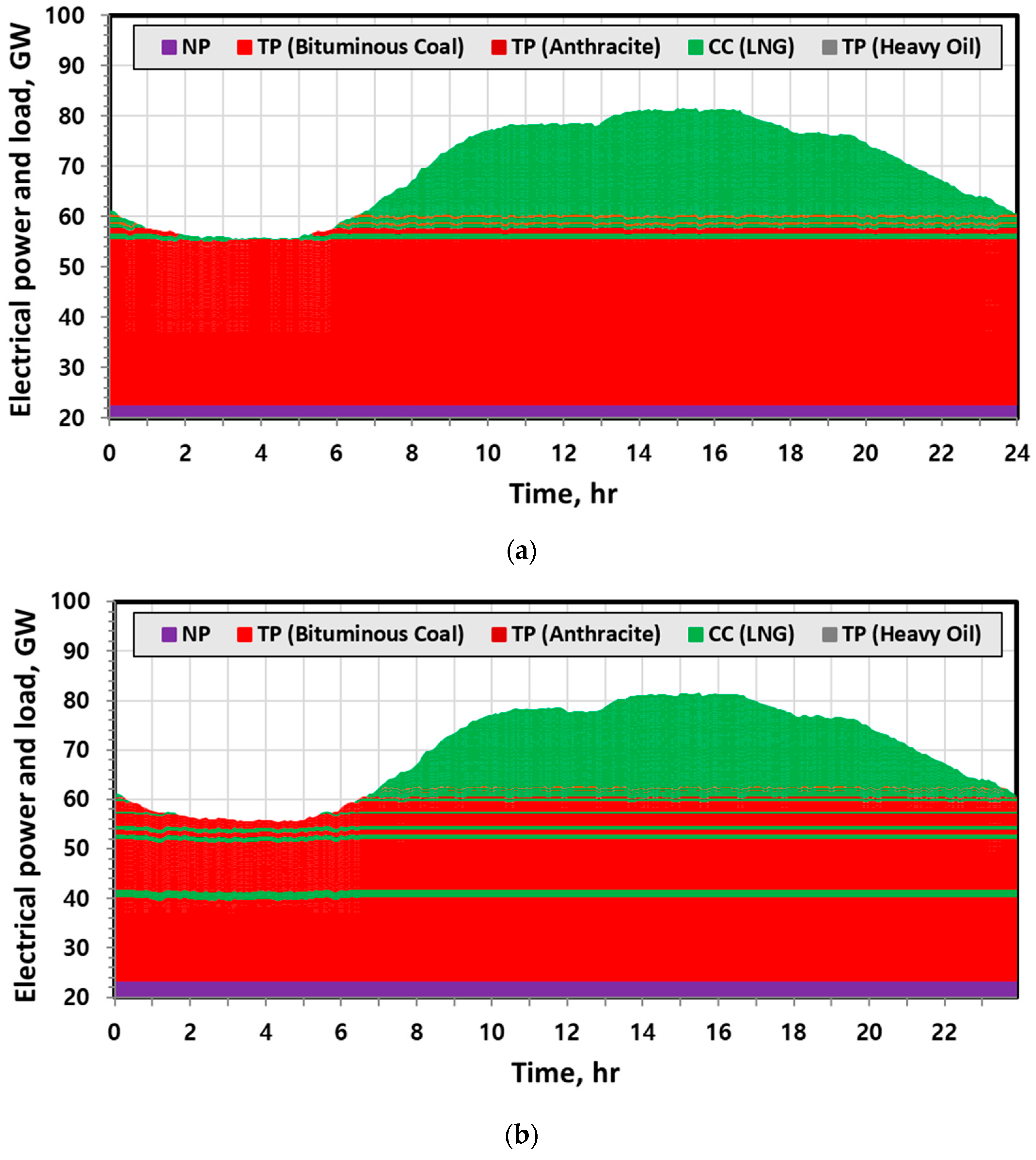
2.1. Centralised Power Plant (CPP) Model

The CPP models consist of turbine and generator modules. There are four model types, as shown in Figure 2: nuclear power plant (NP), thermal power plant (TP), combined-cycle power plant (CC), and pumped-storage hydroelectricity plant (PSH). NP and TP consist of IEEG1; CC has GAST as the gas turbine and CIGRE HRSG/ST as the steam turbine; and PSHP has the HYGOV module as a turbine module [31,32,33]. They are linked to ELGEN, which is a synchronous generator module of ProTRAX [34]. They are dynamic models, in which the turbine and the generator are synchronised; when the turbine and generator are synchronised and connected to the power system, the phase control of the electro-motive force (EMF) phasor is adjusted so that the generator’s electrical output will be the same as the output of the shaft rotating by the turbine; the generator’s free electric power and voltage change according to the change in the EMF vector size; a deviation between the mechanical output and electrical output occurs according to the angular velocity variation.

Table 1. Typical parameter of CPP models [35,36,37].

	NP	TP	TP	CC	PSH
Fuel Type	Nuclear	Coal	Heavy Oil	LNG	Water
Rated capacity (GW)	23.25	35.74	2.95	32.48	3.7
Number (EA)	24	65	13	63	12
Efficiency (%)	33.0~39.0	33.0~42.0	32.0~33.0	42.0~54.0	76.0~82.0
Inertia Constant (s)	6.0~9.0	4.0~7.0	4.0~5.0	3.0~6.0	2.0~4.0
Turbine speed (RPM)	1800	3600	3600	3600	300~600
Droop (%)	-	5~9	4~6	6~8	3~4
Dead band (Hz)	-	±0.0~±0.038	±0.01~±0.03	±0~±0.06	±0.02~±0.033
Ramp rate (%MW/min)	-	0.7~3.1	1.1~2.3	2.6~16.0	22.0~32.0
Heat rate (MBtu/MWh)	9200~10,700	8000~10,900	11,000~11,200	6400~8500	-

shows the typical parameters of the CPP models. The parameters were setuped from the KPX open-API information based on 177 CPP generators in South Korea. The fuel types include nuclear, coal, heavy oil, LNG, and water. In the total capacity of 98.12 GW, NP accounts for 23.7%, TP accounts for 38.68% (Coal-35.74%, Heavy oil-2.95%), CC accounts for 32.48%, and PSH accounts for 3.7%.

To synchronise the turbine’s speed with the frequency of the system measured at the generator, the CPP model performs the governor free (GF), which is a PFC service. The response $P_{PFC.i}$ is calculated using the rated power $P_{rated.i}$, the droop coefficient $K_{droop}$, the generator’s rotating speed ${\omega }_i$ and rated rotating speed ${\omega }_{rated.i}$, as shown in Equation (1).

$$P_{PFC.i}=\frac{P_{rated.i}\left({\omega }_{rated.i}-{\omega }_i\right)}{{\omega }_{rated.i}{K}_{droop}}100 \left[\mathrm{MW}\right]$$

(1)

$K_{droop}$ is configured to be 5% to 9% for TP (coal), 4% to 6% for TP (heavy oil), 6% to 8% for CC, and 3% to 4% for PSH. The CPP’s PFC response section refers to the operation outside the frequency dead-band region, which is configured to be ±0~0.038 Hz for TP (coal), ±0.01~0.03 Hz for TP (heavy oil), ±0~0.06 Hz for CC, ±0.02~0.033 Hz for PSH. The output relationship between the turbine and the generator according to the angular velocity is defined as a swing equation, as shown in Equation (2). The deviation between the turbine output $P_{Mech.i}$ and the generator output $P_{Elec.i}$ is caused by the inertia constant $H_i$, rated capacity $S_{rated.i}$, and angular acceleration, which is the differential of the angular velocity ${\omega }_i$.

$$2H_i{S}_{rated.i}\frac{d\left({\omega }_i/{\omega }_{rated.i}\right)}{dt}=P_{Mech.i}-P_{Elec.i}\left[\mathrm{MW}\right]$$

(2)

The inertia constant $H_i$ is given in seconds and represents the time it takes to fix the rotating generator at the synchronous speed in a state that mechanical power is not supplied, and the rated output is extracted. $H_i$ is 6.0 to 9.0 for NP, 4.0 to 7.0 for TP (coal), 4.0 to 5.0 for TP (heavy oil), 3.0 to 6.0 for CC, and 2.0 to 4.0 for PSH. Therefore, an output deviation occurs depending on the angular speed of the kinetic energy stored in the turbine-generator, which is the product of the inertial constant $H_i$ and the rated capacity $S_{rated.i}$. Because the rotation speed of the synchronised turbine and generator does not vary significantly, it is changed according to the power system’s frequency change, and if a transient state frequency occurs, insufficient power is transferred from the stored kinetic energy, resulting in a decrease in the turbine’s speed.

2.2. Energy Management System (EMS) Model

The EMS Model performs the secondary frequency control (SFC) and the tertiary frequency control (TFC) to maintain the power system’s power and frequency balance, as shown in Figure 3. SFC is carried out by the AGC module, which estimates the power generation of the power grid model’s CPP model and the load of the transmission/substation model and the load model. TFC is performed through the base-point tracking module. The area AGC module that provides the SFC service performs the role of generating a frequency control response every four seconds by measuring the frequency change of a short period in 2-s intervals. The area control error, $ACE$ is calculated through the frequency deviation $\Delta f$ and the system control gain$B$. By calculating the integral of $ACE$, the power system’s total AGC demand $P_{AGC\_Demand}$ is calculated, as shown in Equation (3):

$$P_{AGC\_Demand}={{\displaystyle \int }}^{}ACE={{\displaystyle \int }}^{}10B\left(\Delta f\right)\left[\mathrm{MW}\right]$$

(3)

The AGC participation rate of each CPP is calculated through the ramp rate $K_{ramp.i}$ of the CPP model currently incorporated into the system, and as shown in Equation (4), the AGC response $P_{AGC.i}$ is delivered every four seconds.

$$P_{AGC.i}=P_{AGC\_Demand}\left(\frac{K_{ramp.i}}{{{\displaystyle \sum }}_{i=0}^n{K}_{ramp.i}}\right) \left[\mathrm{MW}\right]$$

(4)

The base point tracking module, which provides the TFC service, responds to the load change over a long period to estimate the load and select a start generator every five minutes and delivers the base point $P_{base.i}$ every one minute. Here, the methods of selecting a start generator are divided into economic load dispatch (EcoLD) and environmental load dispatch (EnvLD) methods. First, the heat rate equation for each CPP model in Table 1 can be shown as Equation (5):

$$H_i\left(P_{base.i}\right)=\frac{a_i}{P_{base.i}}+b_i+c_i{P}_{base.i} \left[\mathrm{MBtu}/\mathrm{MWh}\right]$$

(5)

Here, a fuel cost equation can be created by multiplying the fuel cost $F{C}_i$ and the basepoint $P_{base.i}$. Equation (6) is the fuel cost equation $F_{Eco}$ of EcoLD, and Equation (7) is the fuel cost equation $F_{Env}$ of EnvLD, considering the CO₂ trading price $C_{Co2}$ and the CO₂ emission coefficient $K_{emi}$:

$$F_{Eco}\left(P_{base.i}\right)=\left(c_i{P}_{base.i}{}^2+b_i{P}_{base.i}+a_i\right)\times F{C}_i \left[\$/\mathrm{h}\right]$$

(6)

$$F_{Env}\left(P_{base.i}\right)=\left(c_i{P}_{base.i}{}^2+b_i{P}_{base.i}+a_i\right)\times F{C}_i+\left(C_{Co2}\cdot K_{emi}\right)\times P_{base.i} \left[\$/\mathrm{h}\right]$$

(7)

Through the fuel cost equations, we can find the incremental fuel cost ${\lambda }_i$, which shows the slope of the power output and fuel cost characteristics, as shown in Equation (8):

$${\lambda }_i=\frac{dF\left(P_{base.i}\right)}{d{P}_{base.i}}=2{\alpha }_i{P}_{base.i}+{\beta }_i \left[\$/\mathrm{MWh}\right]$$

(8)

In the case of the CPP model operating with a certain power output, ${\lambda }_i$ represents the incremental fuel cost per unit of time required when the output is increased by 1 MW in this operating state. Therefore, start generators are connected to the power system according to the load in order of the lowest ${\lambda }_i$. In general, in plant power costs, plant operating costs, maintenance and repair costs, and labour costs are all included, but this model only considers pure fuel costs. The cost for each CPP fuel and emission factor were considered according to the EcoLD and EnvLD operation methods for this process, as shown in

Table 2. Average fuel cost and CO₂ emission factor by fuel type.

	NP	TP Bituminous	TP Anthracite	CC LNG	TP Heavy Oil
Fuel Cost ($/MWh)	4.96	44.17	53.35	72.46	141.11
Emission Factor	-	0.8867	0.8867	0.3889	0.6588

, based on which plans of start generators were simulated. Figure 4 shows the results. NP, which has the lowest fuel cost, is responsible for the base load, and the operation start up order is determined in the order of TP (coal), CC (LNG), and TP (heavy oil). In the results of the start up plans, the difference between the two power supply methods is that the incremental fuel cost ${\lambda }_i$ is about 10 to 20 $\$/\mathrm{MWh}$ higher overall in the EnvLD method than in the EcoLD method. It is found that in EnvLD, some CCs, which have good efficiency because of emission factor adjustments, begin to output, starting from a power load of 40 GW.

Based on the power generation start up plan, the generator’s reference output $P_{base.i}$ is calculated in the base point tracking module. This process can satisfy all power loads estimated for the CPPs that have been set up with the start up plan every five minutes, and the control economic/environmental dispatch (CED), which undergoes the minimisation process of the incremental fuel cost ${\lambda }_i$, is performed. After performing CED every minute, the tracking economic/environmental dispatch (TED), which calculates the power output adjustment to respond to the changed load, is performed. This process was implemented using the cvxpy optimization library through the Python API and configured according to Theorem 1. In the CED, constraints are set up through variables and parameters, such as the CPP’s maximum power output $P_{max.i}$ and minimum power output $P_{min.i}$, the incremental fuel cost equation’s coefficients ${\alpha }_i$ and ${\beta }_i$, and the start up state $O{n}_i$ based on the generator’s operation and stop time constraints. Furthermore, $P_{base.i}$ is allocated by performing optimization to minimize the maximum ${\lambda }_i$ among all operating CPPs. The TED performs the power output adjustment according to the load at which the sum of $P_{base.i}$ calculated in CED is estimated. Based on this process, we performed a one-day simulation that allocates $P_{base.i}$ in A1GridSim.

Theorem 1.

Process of optimization for CED and TED by python API.

 1.

Control Economic/Environmental Dispatch

• Import cvxpy as cp
• Import numpy as np
• def Control_ED(n,$P_{load}$, $P_{max}$, $P_{min}$, $\alpha$, $\beta$, $On$):
  • $P_{CED.i}$= cp.variable(shape=n, nonneg=True)
  • ${\lambda }_i$= cp.variable(shape=n, nonneg=True)
  • $P_{max.i}$= cp.parameter(shape=n)
  • $P_{min.i}$= cp.parameter(shape=n)
  • ${\alpha }_i$= cp.parameter(shape=n)
  • ${\beta }_i$= cp.parameter(shape=n)
  • $O{n}_i$= cp.parameter(shape=n)
  • $P_{max.i}$.value = np.array($P_{max}$)
  • $P_{min.i}$.value = np.array($P_{min}$)
  • ${\alpha }_i$.value = np.array($\alpha$)
  • ${\beta }_i$.value = np.array($\beta$)
  • $O{n}_i$.value = np.array($On$)
  •  
  • Constraints = list()
  •  
  • Constraints.append(${\displaystyle \sum }_{i=0}^n{P}_{CED.i}=P_{load}$)
  • Constraints.append($P_{CED.i}\le P_{max.i}\times O{n}_i$)
  • Constraints.append$(P_{CED.i}\ge P_{min.i}\times O{n}_i$)
  • Constraints.append(${\lambda }_i\le 2{\alpha }_i{P}_{CED.i}+{\beta }_i$)
  •  
  • Object = cp.Minimize(max(${\lambda }_1, {\lambda }_2, \cdots , {\lambda }_{n-1}, {\lambda }_n$))
  • Prob = cp.Problem(Object, Constraints)
  • Prob.solve()
  •  
• Return${\lambda }_i$.value,$P_{CED.i}$.value

 2.

Tracking Economic/Environmental Dispatch

• def Traking_ED($P_{load}$, ${\lambda }_i$, ${\displaystyle \sum }_{i=0}^n{P}_{CED.i}$):
  • If $P_{load}-{\displaystyle \sum }_{i=0}^n{P}_{CED.i}>0$:
  • $P_{TED.i}=\left(P_{load}-{\displaystyle {\displaystyle \sum }_{i=0}^n}{P}_{CED.i}\right)\times \frac{{\lambda }_i}{{{\displaystyle \sum }}_{i=0}^n{\lambda }_i}$$elseif$ $P_{load}-{\displaystyle \sum }_{i=0}^n{P}_{CED.i}<0$:
  • $P_{TED.i}=\left(P_{load}-{\displaystyle {\displaystyle \sum }_{i=0}^n}{P}_{CED.i}\right)\times \frac{\frac{1}{{\lambda }_i}}{{{\displaystyle \sum }}_{i=0}^n\frac{1}{{\lambda }_i}}$Return $P_{TED.i}$.value

Figure 5 shows the one-day simulation result based on the base-point tracking mode. It shows the power generation situations layered in the start up order defined by the power generation start up plan. In the overall trend, it is found that power is generated in the order of NP, TP (coal), CC, and TP (heavy oil). The biggest difference between EcoLD and EnvLD, as shown in the start up plan, is that NP and TP (coal) account for the majority of EcoLD below 55 GW, whereas CCs, which have high efficiency due to the emission factor, are operated for base power generation starting at 40 GW in EnvLD. As such, the EMS model performs the SFC in the area AGC module in a short period and performs the TFC in the base-point tracking module in a long period to balance the power generation demands and maintain the quality of the power frequency. This means that the EMS model includes the centralised frequency control system that operates in the actual EMS. Furthermore, when it is performed according to the power generation start up plan and the base-point tracking mode, considering the dynamic characteristics of CPP, it shows the characteristics of the national power grid, in which the CPP models that have different inertia characteristics depending on the changing load characteristics are connected to the system and operated.

2.3. Dynamic Frequency Model

The dynamic frequency model is a frequency model that has dynamic characteristics according to the power generation and demand. It is possible to approximate the relationship between the CPP model’s turbine and generator by creating a kinetic equation of all parallel generators in the current power system, such as Equation (2). It can be represented approximately as Equation (9):

$${\displaystyle \sum }_{i=0}^n\frac{2H_i{S}_i}{f_{rated}}\frac{d{f}_{sys}}{dt}={\displaystyle \sum }_{i=0}^n{P}_{Mech.i}-{\displaystyle \sum }_{i=0}^n{P}_{Elec.i}\left[\mathrm{MW}\right]$$

(9)

Equation (9) shows the deviation between ${\displaystyle \sum }_{i=0}^n{P}_{Mech.i}$ (the sum of $P_{Mech.i}$, which is the output of the turbine) and ${\displaystyle \sum }_{i=0}^n{P}_{Elec.i}$ (the sum of $P_{Elec.i}$, which is the output of the generator) causes a change in the power system frequency $f_{sys}$. Furthermore, general resistance load is not related to frequency but has the self-control characteristics, in which the power consumption changes according to the change in frequency in proportion to the rotational speed at the rotator load, as shown in Equation (10):

$$K_L\Delta f=\frac{\%K_L\cdot P_{Load}}{10}\Delta f\left[\mathrm{MW}\right]$$

(10)

It is obtained using the load constant $K_L$ [MW/0.1 Hz] and the frequency deviation $\Delta f$. $K_L$ is obtained using $\%K_L$ of a 0.2–0.6% range and the total load $P_{Load}$. $\Delta f$ is obtained as the deviation between $f_{sys}$ and $f_{rated}$(60 Hz).

Therefore, Equation (11) can represent the characteristics of the power frequency based on the CPP Model’s inertia characteristics and the load’s self-control characteristics.

$${\displaystyle \sum }_{i=0}^n\frac{2H_i{S}_{rated.i}}{f_{rated}}\frac{d{f}_{sys}}{dt}+K_L\Delta f=\Delta P_{sys}\left[\mathrm{MW}\right]$$

(11)

It can be seen that the power deviation occurs due to the deviation of the turbine-generator output caused by the frequency change and the load’s self-control characteristics. If Laplace transform is applied to this, the relationship between the power deviation $\delta$ and frequency deviation $\phi$ can be represented by Equation (12):

$$\frac{\phi }{\delta }={\left({\displaystyle \sum }_{i=0}^n\frac{2H_i{S}_{rated.i}}{f_{rated}}s+K_L\right)}^{-1}\left[\mathrm{Hz}/\mathrm{MW}\right]$$

(12)

where the power system’s proportional gain $K_F$ and the frequency time constant $T_F$ can be obtained by Equations (13) and (14):

$$K_F=\frac{1}{K_L}\left[\mathrm{Hz}/\mathrm{MW}\right]$$

(13)

$$T_F={\displaystyle \sum }_{i=0}^n\frac{2H_i{S}_{rated.i}}{f_{rated}{K}_L}\left[\mathrm{s}\right]$$

(14)

The power system’s proportional gain $K_F$ is determined by the change in the power load according to the load constant $K_L$. The frequency time constant $T_F$ is determined by the load constant $K_L$ and the kinetic energy stored in the CPP model incorporated according to the generator start up plan.

If 24-h simulation of the dynamic frequency model is performed using the CPP model, EMS model, and power grid model examined so far, we can obtain results such as those shown in Figure 6. Figure 6 shows the results of performing the 24-h simulation using power load data from December 2019. For loads of 55.401 GW minimum and 81.535 GW maximum, the power generation output is operated from 55.393 GW minimum to 81.454 GW maximum. In general, the base load is shown between 00:00 and 06:00, and the peak load is shown between 12:00 and 18:00. Accordingly, the frequency deviation is −0.012 to +0.037 Hz in the base load period and −0.062 to +0.049 in the peak load period.

2.4. BESS System Model

The BESS model is constructed based on the control algorithm and hardware control system developed in the “Frequency regulation control for BESS” project led by the Korea Electric Power Corporation [38,39,40], and its target was the BESS of 380 MW/111 MWh installed in substations across the country. Figure 7 shows the status of BESS for PFC installed on A1GridSim. In total, 376 MW PCS and 103 MWh batteries have been installed at 13 substations on the mainland, and 4 MW PCS and 8 MWh batteries have been installed on Jeju Island. A typical BESS consists of one FRC and four PCS/ESS sets, though this varies by substation. The hardware hierarchical multi-system of the BESS for PFC has a structure of the master power management system (MPMS), Local power management system (LPMS), Frequency regulation control master (FRCM), FRC, PCS, and BESS. The FRC and FRCM are referred to as the LPMS, and their role is to coordinate the FRC’s participation rate. MPMS is a hierarchical layer for the integrated operation of LPMS at the substation level. The virtual physical model’s PCS/BESS is physically linked to the power grid model, and the discrete models, such as the operation sequence of PCS, are constructed as emulation models in linkage with FRC. The FRC’s control algorithm is simulated in linkage with the PCS/ESS model in the SILS mode. In the HILS mode, the simulation is performed by linking the actual FRC hardware controller with a communication model, such as DNP3.0 or Modbus.

3. Software in the Loop Simulation for BESS System

In this section, we will examine the performance of the PFC algorithm considering PRDT, based on the SILS mode of A1GridSim. To this end, Section 3.1 shows the results comparatively verifying the actual transient state frequency history data and the A1GridSim’s transient state simulation frequency. Section 3.2 performs transient state simulations to compare the case of no BESS and the cases of PRDT being 140 ms, 160 ms, and 180 ms and shows the results of analysing the effects of operating PFC and analysing the trajectories of the system characteristics by physical delay time. Finally, Section 3.3 analyses the system characteristic trajectories for each PRDT from 140 ms to 640 ms in 20 ms increments and shows the results of the comparative analysis of the major characteristics.

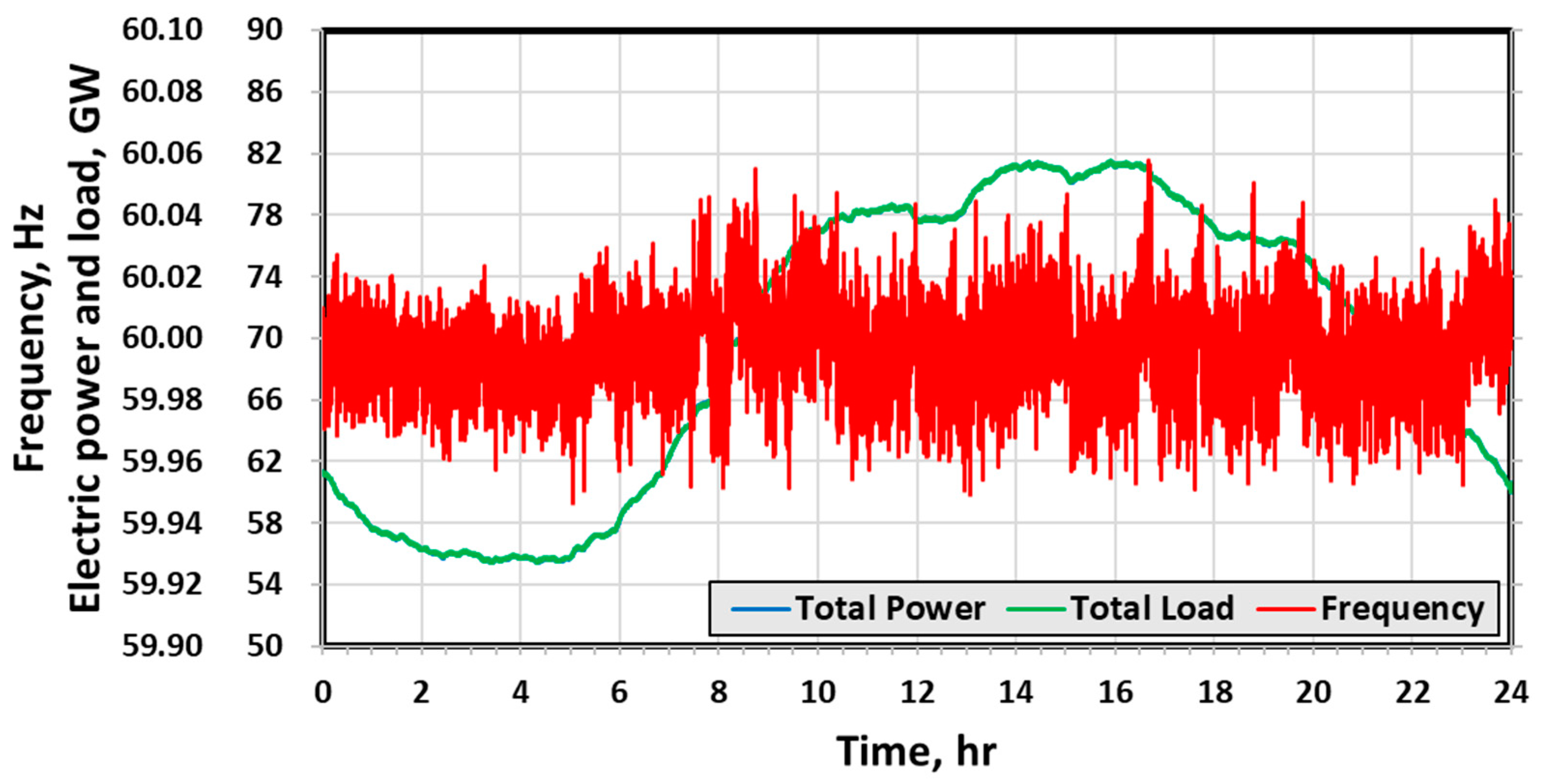
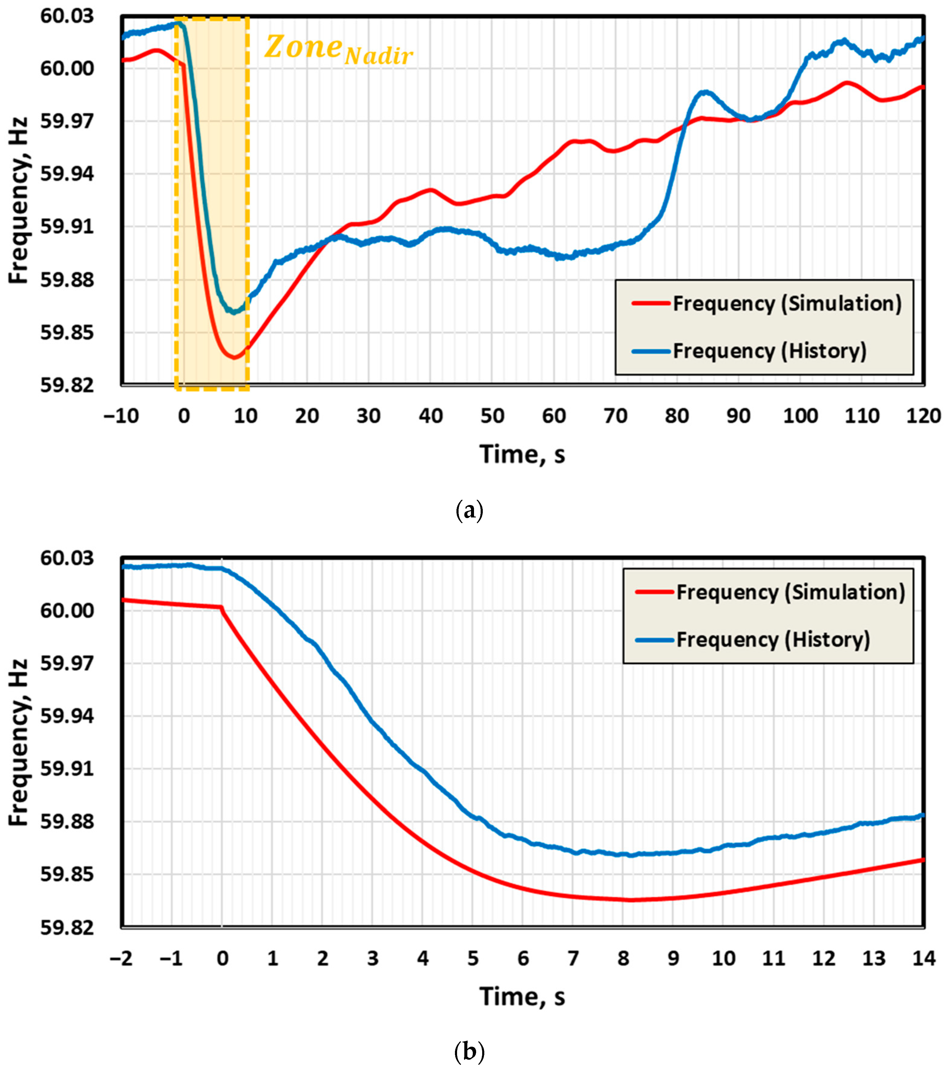
3.1. Verification of Dynamic Frequency Model

To verify the dynamic frequency model of A1GridSim, a real-time dynamic simulation that includes the national power grid model, we conducted a comparative analysis using the frequency transient state history data. The frequency transient state history data target is the data of the frequency transient state caused by the halting incident of one 950 MW nuclear power generator during the peak load time at 3:00 p.m. in August 2016. In the simulation environment, too, the same load data were entered to simulate the halting incident of one 950 MW nuclear power generator where the CPP model is operated by the EMS model. Figure 8 shows the actual historical data and the simulation results. Real refers to the actual frequency history data, and History refers to the history of actual situations.

In history, a frequency drop of 0.1632 Hz occurred, and it took 8.16 s to reach the nadir frequency point. In the simulation, a frequency drop of 0.1648 Hz occurred, and it took 7.88 s to reach the nadir frequency point. When we examined the average RoCoF up to the nadir point in the state just before the incident, we found that it was 0.0207 Hz/s in Real and 0.0202 Hz/s in Sim. When the error rates were examined, it was found that the error rate was 0.9% in the frequency drop, 3.5% in the time consumed to reach the nadir point, and 2.48% in the average RoCoF, showing there is a high degree of similarity in the transient state.

3.2. Performance Verification of the BESS System for PFC

In this subsection, to examine the performance of the BESS for PFC, we simulate a halting incident of one 950 MW generator in a situation where the frequency change is the largest in the low-inertia system. To this end, we conducted case studies by configuring a case where the transient state is recovered with the CPP model alone without deploying the BESS and cases in which the PRDT is 140 ms, 160 ms, and 180 ms. Figure 9 shows the results of case studies in terms of RoCoF, BESS power, and CPP’s GF response.

In Figure 9, (a) shows the frequency, (b) shows RoCoF, (c) shows the BESS power, and (d) shows the GF response. The main results of Figure 9 are summarised in

Table 3. Summary of simulation results from the several case studies.

	No BESS (Case1)	140 ms (Case2)	160 ms (Case3)	180 ms (Case4)
$f_{initial}$	59.9914	59.9914	59.9914	59.9914
$T_{nadir}$	3.04	2.84	2.82	2.80
$f_{nadir}$	59.8401	59.8954	59.8952	59.8951
$\Delta f_{nadir}$	0.1599	0.1046	0.1048	0.1049
$RoCo{F}_{average}$	0.05259	0.0368	0.0372	0.0375
$RoCo{F}_{BESS}$	-	−0.0510	−0.0505	−0.0500
$GF{R}_{max}$	893.86	535.02	538.72	539.11
$T_{recovery}$	105.1	150.2	150.2	150.2

. When the results of BESS cases are compared to the case of No BESS as a reference case, the time for reaching the nadir frequency point, $T_{\mathrm{Nadir}}$, decreased by 6.58%, 7.24%, and 7.89% in the cases, respectively. Meanwhile, the frequency deviation ${\Delta \mathrm{f}}_{\mathrm{Nadir}}$ decreased by 34.58%, 34.46%, and 34.40%, respectively. When the average RoCoF is calculated using ${\Delta \mathrm{f}}_{\mathrm{Nadir}}$ and $T_{\mathrm{Nadir}}$, the result is 0.0526 Hz/s, 0.0368 Hz/s, 0.0372 Hz/s, and 0.0375 Hz/s in Cases 1 to 4, respectively. As many previous studies have shown, it is found that ${\Delta \mathrm{f}}_{\mathrm{Nadir}}$ and the average RoCoF are greatly improved in the cases of having the BESS for PFC compared to the case of No BESS. Furthermore, as shown in the simulation results of BESS power in Figure 9c, ${\Delta \mathrm{f}}_{\mathrm{Nadir}}$ and the average RoCoF improve as the PRDT becomes faster. Finally, the time for recovering to the rated frequency $f_{\mathit{rated}}$ is 30% faster for No BESS, but in the case of No BESS, an overshooting phenomenon occurs in the process of recovering to $f_{\mathit{rated}}$, showing that it takes about 20% longer time compared to the case of having BESS.

When the instantaneous RoCoF in the transient state is examined, it is found that the minimum RoCoF to reach $f_{\mathrm{Nadir}}$ is −0.0958 Hz/s in every case. The reason is that it is the result before the BESS system responds. Therefore, when it is examined at the respective response time of the BESS (Cases 2 to 4), it is −0.051 Hz/s, −0.0505 Hz/s, and −0.05 Hz/s, respectively, which means the BESS responds faster as the RoCoF decreases. Lastly, ${\mathit{GFR}}_{\mathit{max}}$, the CPP’s GR response value, has decreased by 40.14%, 37.73%, and 39.69% in the cases of having BESS compared to the case of No BESS.

The results of the case studies examined so far were analysed through the system characteristic trajectory according to each case. In the transient state of the entire system, the trajectory was tracked with the relationship between the power deviation $\Delta P_{trn}$ and the frequency deviation $\Delta f_{trn}$. $\Delta P_{trn}$ and $\Delta f_{trn}$ were calculated by Equation (15) and (16):

$$\Delta P_{trn}=\left(\frac{P_{Gen}{}^t-P_{Gen}{}^{t=0}}{P_{Gen}{}^{t=0}}\right)-\left(\frac{P_{Load}{}^t-P_{Load}{}^{t=0}}{P_{Load}{}^{t=0}}\right)\left[\mathrm{pu}\right]$$

(15)

$$\Delta f_{trn}=\frac{f_{sys}{}^t-f_{sys}{}^{t=0}}{f_{sys}{}^{t=0}} \left[\mathrm{pu}\right]$$

(16)

Figure 10 shows the relationship between the power deviation and the frequency deviation in the frequency transient state, and shows the trajectory of the power grid constant. The power grid constant can be shown by Equation (17) according to the relationship between the two:

$$K_{sys}=\frac{\Delta P_{trn}}{\Delta f_{trn}}$$

(17)

In Figure 10, (a) shows the power grid constant over the entire period, (b) shows the response point of the BESS, (c) shows the nadir frequency point, (d) Quasi-steady state point, and (e) shows the overshooting region of the frequency control in the region where the rated frequency is reached. If the generator halts at a point where the power distribution and frequency deviation are both 0 pu, the power deviation decreases sharply to −0.0215 pu, after which a frequency deviation occurs. As shown in Figure 9, every case follows the same power grid constant before the BESS responds. At the point where the BESS responds, the decrease in the power and frequency deviations is temporarily reduced, as shown in Figure 10b. After this, it proceeds to the nadir frequency point, and as shown in Figure 10c, it reaches the peak point of frequency deviation. Here, the power grid constant is 0.946, 0.891, 0.893, and 0.898 in Cases 1 to 4, respectively. These points are Points where the rated frequency is recovered from the nadir frequency, and as the value of the power grid constant decreases, the recovering ability increases. The BESS is operating at its maximum power output of 376 MW, and from the point of recovery by the CPP’s GF response, the next point, the quasi-steady state, can be reached with a relatively smaller GF response as the power grid constant decreases. This is the reason why $GF{R}_{\mathit{max}}$ is small in the case of the BESS with a fast PRDT. Next, Figure 10d shows the region for reaching the quasi-steady state through the nadir frequency point. In the presence of a power deviation, the power deviation is positive because the power generation exceeds the load, and the frequency change in the transient state is converged to 0, allowing the quasi-steady state point to be reached. The power grid constant at the quasi-steady state point is 0.935, 0.784, 0.782, and 0.779, respectively. In this region, a transient state occurs, and a stable state is maintained primarily. As the power grid constant increases, it can be shown that the stability increases in the frequency change. Here, the case of No BESS has the highest value because it is in a state where very high GF and AGC responses are incorporated into the power grid, which later causes the overshooting at the transient state recovery point. Finally, Figure 10e shows that the recovery has been achieved, as it was before the transient state occurred. In the case of No BESS, overshooting occurs, but in the case of applying the BESS, the overshooting phenomenon is inhibited through immediate charging control.

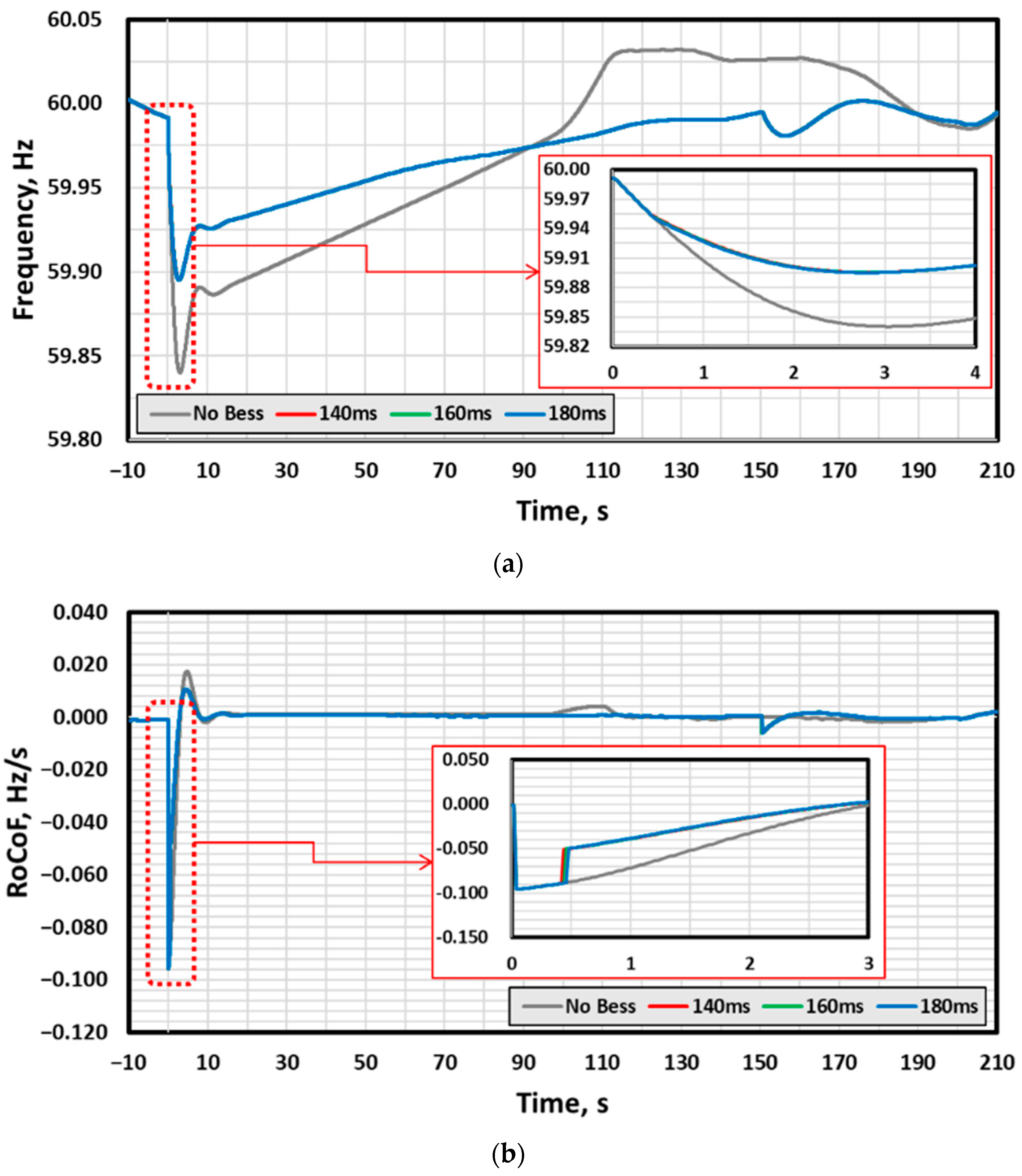
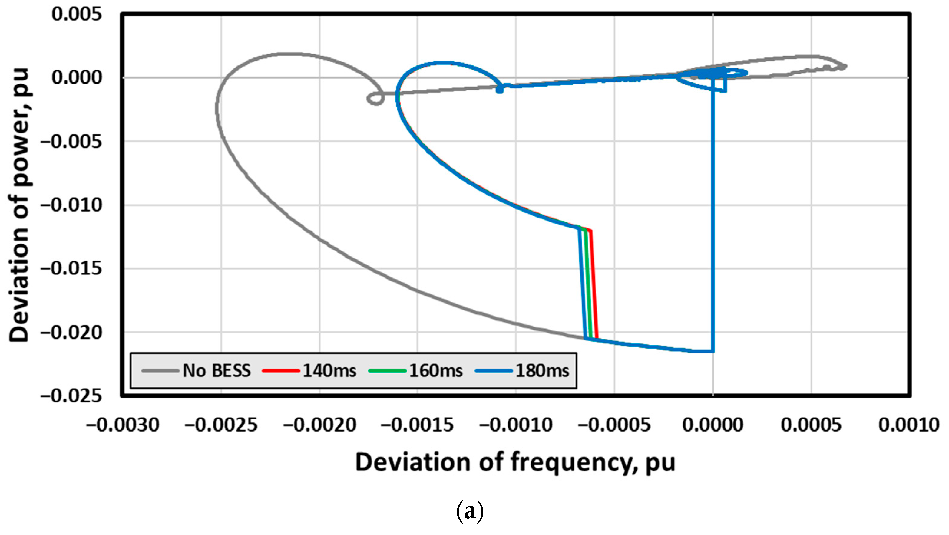
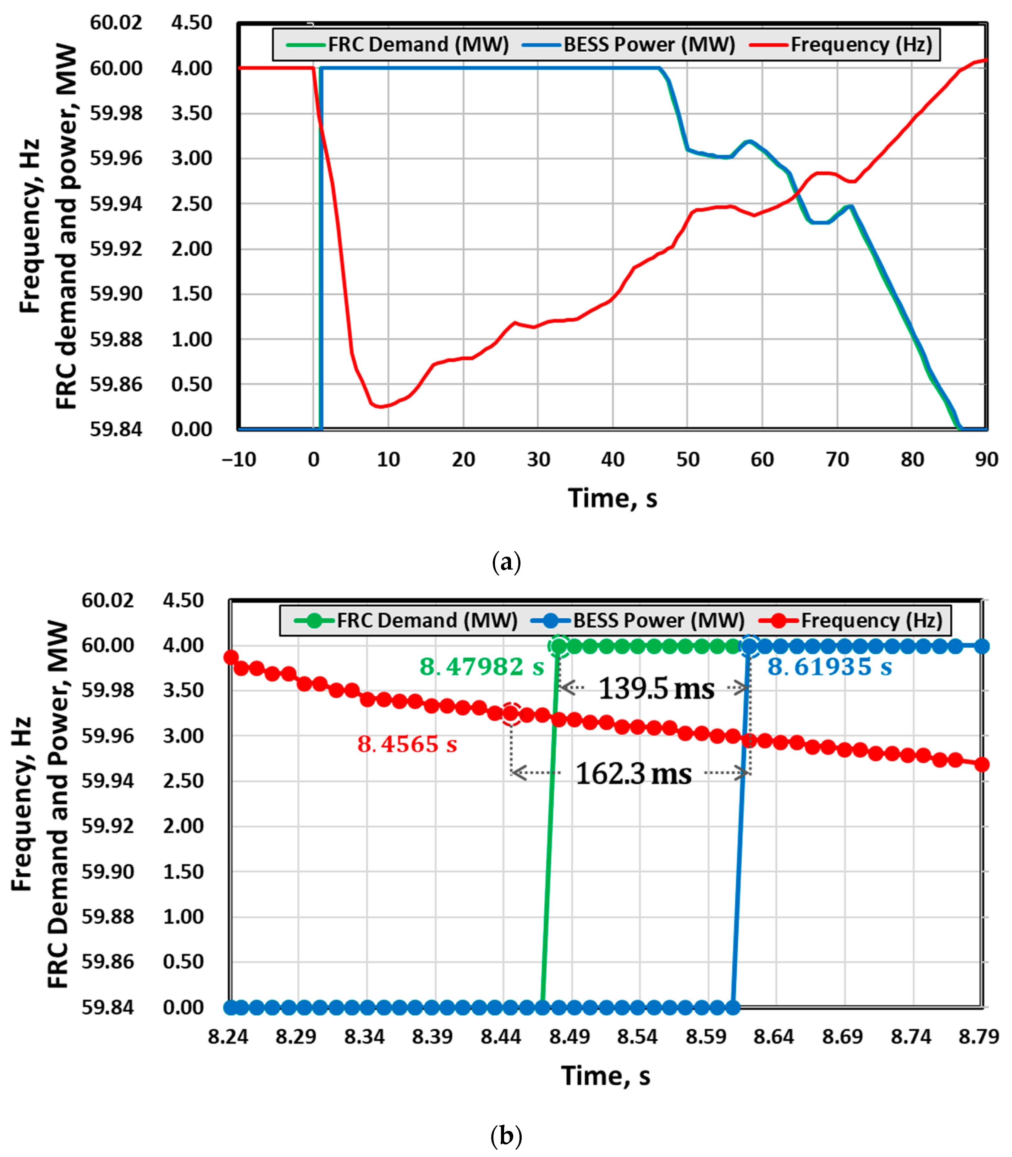
3.3. Analysis of Impact on Physical Response Delay Time between FRC and PCS

We have examined the performance verification results of the BESS for PFC above. Here, we have found that the faster the PRDT, the better the transient state recovery performance. As shown in the results of Figure 9 and Figure 10, there is no large difference between the cases of 140 ms and 180 ms in the case studies. As a result, in this subsection, we will examine the main results by analysing the trajectories, as in Section 3.2, for the results from 140 ms, where the system can respond most quickly due to hardware characteristics, to 640 ms in 20 ms intervals.

Figure 11 shows the main results of analysing the trajectory at the transient state frequency according to the PRDT. It shows (a) the power grid constant at the nadir frequency point, (b) nadir frequency, (c) average RoCoF, (d) GF response when the BESS responds, and (e)${\mathit{GFR}}_{\mathit{max}}$. At the point where the frequency is recovered after the maximum drop of the frequency at the nadir frequency point, the quasi-steady state can be recovered more stably as the power grid constant decreases. In case of PRDT of 200 ms, the power grid Constant is 0.86198, which is 4% lower than that of the case where the PRDT is faster than 180 ms. As explained earlier, as the PRDT increases, the power grid constant at the nadir frequency point decreases, in which case the quasi-steady state can be stably reached. However, this must be checked with the trajectories of frequency, RoCoF, and GF response. As confirmed earlier, the nadir frequency and the average RoCoF decrease as the PRDT increases. When the GF response is examined, it is found that the GF response at the BESS response point increases after 200 ms, and finally, ${\mathit{GFR}}_{\mathit{max}}$ also increases. Therefore, the reason why the power grid constant at the nadir frequency point starts to decrease at 200 ms is that the power deviation decreases since the GR response rate for the BESS response is larger than that of the case faster than 200 ms. This means that the BESS responds faster than the CPP’s PFC, reducing the CPP’s GF response, and the goal of quickly inhibiting the frequency drop is not met due to the slow response time. This means that the PRDT faster than 200 ms must be maintained to use the performance of the BESS as much as possible.

4. Hardware in the Loop Simulation for BESS System

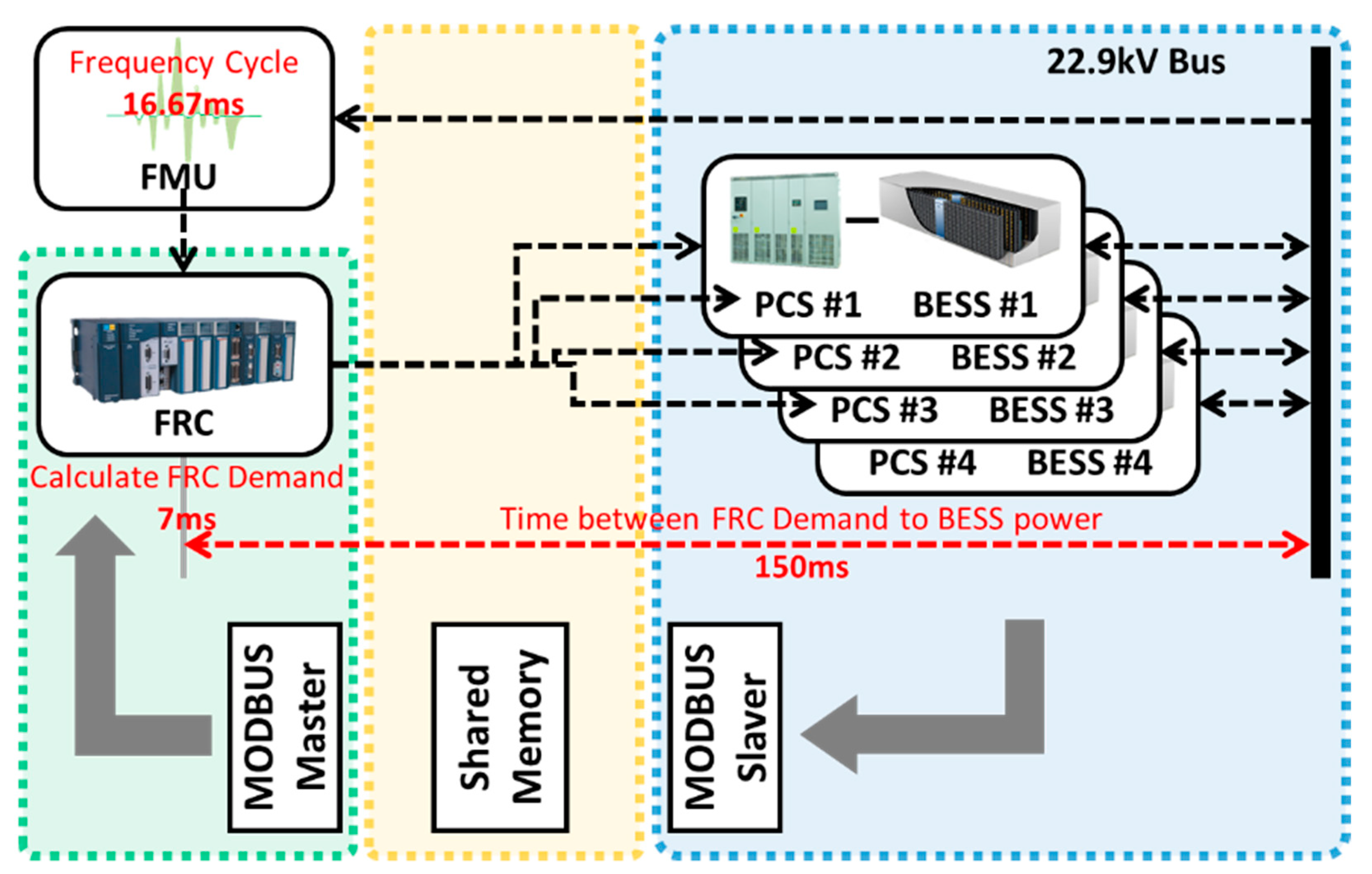
4.1. Configuration of the HILS System for Response Performance Evaluation

For HILS, we constructed the PCS-BESS in the BESS for PFC as a cyber physical model and linked it to the real FRC to evaluate the optimal PRDT performance. Figure 12 shows the configuration and characteristics of the actual and virtual BESS. The actual BESS measures the frequency of the power grid in 16.67 ms cycles through the frequency measurement unit (FMU) and sends it to the FRC. It takes 7 ms to generate the FRC demand based on this frequency and 150 ms to generate the BESS power through the demand received from the FRC. Through this system, the PRDT of 180 ms or less should be satisfied, as the result of SILS. To implement such a real hardware hierarchical multi-system as a CPS, we constructed the PCS, BESS, and power grid systems as physical models and linked them to the real FRC. The communication model was configured with MODBUS, a protocol that links the real FRC and the PCS, and a shared memory was configured so that the respective PCS-BESS processes can access the FRC simultaneously. Here, for the electric power grid model and the BESS model, the calculations were performed in time-steps of 16.625 ms so that the response level would be the same as that of the real facility. These configurations were implemented with portable test equipment that can check the response performance of the FRC installed at the substations, and the performance test was conducted.

4.2. Result of BESS’s Response Performance Evaluation by HILS

Figure 13 shows the response experiment results of the FRC at Non-gong Substation, which were checked through the Iba analyser, a process data acquisition system. For this, we constructed virtual physical models for the 36 MW PCS and 9 MWh batteries of Non-gong Substation to conduct the response performance test. As shown in Figure 13a, the frequency transient state simulation was performed for about 90 s, and the nadir frequency became 59.8501 Hz at 8.91 s. To gain a more detailed view of the time that the BESS responded, we examined the BESS response point, as shown in Figure 13b. At 8.45650 s, the frequency dead-band was deviated, and the FRC determined the frequency transient state. At 8.47928 s, an FRC demand was generated, and at 8.61935 s, the BESS power responded.

Therefore, it took 23.32 ms to generate the FRC demand according to the frequency change, and it took 139.5 ms for the BESS power to respond after the generation of the FRC demand. As a result, 162.3 ms was required for the PRDT, which was the time taken while the FRC determined the frequency, and finally, the BESS responded. As such, through the HILS, it was confirmed that the PRDT response performance was sufficiently satisfied for the FRC of the on-site BESS.

5. Summary Results

In this study, we used the SILS and HILS to provide the performance verification and evaluation results of the BESS. In the SILS type, compared to the frequency history data, the error rate in the maximum drop frequency was 0.9%, the error rate in the time consumed to reach the nadir frequency was 3.5%, and the average RoCoF was 2.45, confirming a high level of reliability. Furthermore, comparative analysis was performed between the cases of recovering without the BESS for PFC in a frequency transient state caused by a halting incident of a 950 MW generator and the case of PRDT of 140 ms, 160 ms, and 180 ms in a 376 MW BESS. The results showed that the maximum frequency drop was reduced by 34.40 to 34.58% in the case of having the BESS for PFC compared to the case of No BESS. Furthermore, the time taken to reach the nadir frequency point was reduced by 6.58 to 7.89%, and the average RoCoF was reduced by 28.70 to 30.03%. Therefore, it was confirmed that the frequency drop inhibition in the transient state was improved. Meanwhile, the CPP’s GF response decreased by 37.73 to 40.14%. Furthermore, the power grid’s constant trajectory was tracked in the frequency transient state. In the case of adding the BESS for PFC, the power grid constant at the nadir frequency point was reduced by 5.07 to 5.81%, and the ability to recover to the quasi-steady state was greatly improved. In addition, we conducted the trajectory analysis with a PRDT of 140 ms to 640 ms to examine the power grid constant, nadir frequency, RoCoF, and GF response at the nadir frequency point. In the results, as the PRDT decreased, the nadir frequency decreased, and the RoCoF’s decrease rate increased, while the power grid constant started to decrease greatly at 200 ms. This is because the GF response trend at the BESS response point starts to decrease at 200 ms, and as the maximum GF response’s increase rate increases, the change in the power deviation decreases relative to the frequency deviation, and the power grid constant decreases, thus reducing the inhibition of the frequency drop. Therefore, when examined comprehensively, it is found that when a PRDT faster than 180 ms is satisfied, the GF response reduction effect increases, improving the power system’s stability. The HILS-type simulation was designed to mitigate the communication load with the FRC through the shared memory to verify the optimal response performance of the BESS installed at actual substations, and the performance test results showed that the PRDT was 162.3 ms, which satisfied the requirement.

6. Conclusions

This study introduced a novel power grid simulation with the BESS model for PFC. It is a real-time dynamic simulator that has a national power grid model, based on which real-time simulations can be performed in time-steps ranging from several ms to tens of ms. The continuous characteristics of the models can be analysed in real-time by analysing the characteristic trajectories of the power system at the national power grid level, based on the dynamic CPP model, the EMS models of PFC, SFC, and TFC, and the dynamic frequency model according to the power generation type, which are the key models. We presented the results of verifying the performance of the BESS algorithm for PFC and evaluating the response performance of the hardware controller based on these characteristics.

As result, it was confirmed that when BESS was used in the frequency transient state, the maximum frequency drop, the RoCoF, and the GF response of CPP were improved by about 30% than No BESS. In addition, the PRDT also confirmed that performance can be satisfied only when it reacts faster than up to 180 ms, and that the response performance of HILS’ hardware controller is satisfied at 162.3 ms.

These functions of the CPS simulator can be used as an evaluation platform for solutions, such as a virtual power plant consisting of hardware hierarchical multi-systems. To this end, we need to develop reliable models for distributed power sources consisting of various energy sources and variable types of communication protocol models to ensure scalability.

References

1. Tremblay, O.; Dessaint, L.-A. Experimental validation of a battery dynamic model for EV applications. World Electr. Veh. J. 2009, 3, 289–298. [Google Scholar] [CrossRef] [Green Version]
2. Zhang, Y.; Lyden, S.; de la Barra, B.L.; Haque, M.E. Optimization of Tremblay’s battery model parameters for plug-in hybrid electric vehicle applications. In Proceedings of the 2017 Australasian Universities Power Engineering Conference (AUPEC), Melbourne, VIC, Australia, 19–22 November 2017; pp. 1–6. [Google Scholar]
3. Surya, S.; Channegowda, J.; Datar, S.D.; Jha, A.S.; Victor, A. Accurate battery modeling based on pulse charging using MATLAB/Simulink. In Proceedings of the 2020 IEEE International Conference on Power Electronics, Drives and Energy Systems (PEDES), Jaipur, India, 16–19 December 2020; pp. 1–3. [Google Scholar]
4. Xia, Q.; Yang, D.; Wang, Z.; Ren, Y.; Sun, B.; Feng, Q.; Qian, C. Multiphysical modeling for life analysis of lithium-ion battery pack in electric vehicles. Renew. Sustain. Energy Rev. 2020, 131, 109993. [Google Scholar] [CrossRef]
5. Fan, X.; Zhang, W.; Wang, Z.; An, F.; Li, H.; Jiang, J. Simplified battery pack modeling considering inconsistency and evolution of current distribution. IEEE Trans. Intell. Transp. Syst. 2020, 22, 630–639. [Google Scholar] [CrossRef]
6. Dubarry, M.; Baure, G.; Pastor-Fernández, C.; Yu, T.F.; Widanage, W.D.; Marco, J. Battery energy storage system modeling: A combined comprehensive approach. J. Energy Storage 2019, 21, 172–185. [Google Scholar] [CrossRef]
7. Tan, R.H.; Tinakaran, G.K. Development of battery energy storage system model in MATLAB/Simulink. Int. J. Smart Grid Clean Energy 2020, 9, 180–188. [Google Scholar] [CrossRef]
8. Rancilio, G.; Lucas, A.; Kotsakis, E.; Fulli, G.; Merlo, M.; Delfanti, M.; Masera, M. Modeling a large-scale battery energy storage system for power grid application analysis. Energies 2019, 12, 3312. [Google Scholar] [CrossRef] [Green Version]
9. Jo, H.; Choi, J.; Agyeman, K.A.; Han, S. Development of frequency control performance evaluation criteria of BESS for ancillary service: A case study of frequency regulation by KEPCO. In Proceedings of the 2017 IEEE Innovative Smart Grid Technologies–Asia (ISGT–Asia), Auckland, New Zealand, 4–7 December 2017; pp. 1–5. [Google Scholar]
10. Sanduleac, M.; Toma, L.; Eremia, M.; Boicea, V.A.; Sidea, D.; Mandis, A. Primary frequency control in a power system with battery energy storage systems. In Proceedings of the 2018 IEEE International Conference on Environment and Electrical Engineering and IEEE Industrial and Commercial Power Systems Europe (EEEIC/I&CPS Europe), Palermo, Italy, 12–15 June 2018; pp. 1–5. [Google Scholar]
11. Stein, K.; Tun, M.; Matsuura, M.; Rocheleau, R. Characterization of a fast battery energy storage system for primary frequency response. Energies 2018, 11, 3358. [Google Scholar] [CrossRef] [Green Version]
12. Bang, H.; Aryani, D.R.; Song, H. Application of battery energy storage systems for relief of generation curtailment in terms of transient stability. Energies 2021, 14, 3898. [Google Scholar] [CrossRef]
13. Meng, Y.; Li, X.; Liu, X.; Cui, X.; Xu, P.; Li, S. A Control Strategy for Battery Energy Storage Systems Participating in Primary Frequency Control Considering the Disturbance Type. IEEE Access 2021, 9, 102004–102018. [Google Scholar] [CrossRef]
14. Izadkhast, S.; Cossent, R.; Frías, P.; García-González, P.; Rodríguez-Calvo, A. Performance Evaluation of a BESS Unit for Black Start and Seamless Islanding Operation. Energies 2022, 15, 1736. [Google Scholar] [CrossRef]
15. Abayateye, J.; Corigliano, S.; Merlo, M.; Zimmerle, D. BESS Primary Frequency Control Strategies for the West Africa Power Pool. Energies 2022, 15, 990. [Google Scholar] [CrossRef]
16. Schiapparelli, G.P.; Massucco, S.; Namor, E.; Sossan, F.; Cherkaoui, R.; Paolone, M. Quantification of primary frequency control provision from battery energy storage systems connected to active distribution networks. In Proceedings of the 2018 Power Systems Computation Conference (PSCC), Dublin, Ireland, 11–15 June 2018; pp. 1–7. [Google Scholar]
17. Zhu, D.; Zhang, Y.-J.A. Optimal coordinated control of multiple battery energy storage systems for primary frequency regulation. IEEE Trans. Power Syst. 2018, 34, 555–565. [Google Scholar] [CrossRef]
18. Toma, L.; Sanduleac, M.; Baltac, S.A.; Arrigo, F.; Mazza, A.; Bompard, E.; Musa, A.; Monti, A. On the virtual inertia provision by BESS in low inertia power systems. In Proceedings of the 2018 IEEE International Energy Conference (ENERGYCON), Limassol, Cyprus, 3–7 June 2018; pp. 1–6. [Google Scholar]
19. Choi, W.Y.; Kook, K.S.; Yu, G.R. Control strategy of BESS for providing both virtual inertia and primary frequency response in the Korean Power System. Energies 2019, 12, 4060. [Google Scholar] [CrossRef] [Green Version]
20. Pinthurat, W.; Hredzak, B. Decentralized Frequency Control of Battery Energy Storage Systems Distributed in Isolated Microgrid. Energies 2020, 13, 3026. [Google Scholar] [CrossRef]
21. Obaid, Z.A.; Cipcigan, L.; Muhssin, M.T.; Sami, S.S. Control of a population of battery energy storage systems for frequency response. Int. J. Electr. Power Energy Syst. 2020, 115, 105463. [Google Scholar] [CrossRef]
22. Amin, M.R.; Negnevitsky, M.; Franklin, E.; Alam, K.S.; Naderi, S.B. Application of battery energy storage systems for primary frequency control in power systems with high renewable energy penetration. Energies 2021, 14, 1379. [Google Scholar] [CrossRef]
23. Manbachi, M.; Sadu, A.; Farhangi, H.; Monti, A.; Palizban, A.; Ponci, F.; Arzanpour, S. Real-time co-simulation platform for smart grid volt-VAR optimization using IEC 61850. IEEE Trans. Ind. Inform. 2016, 12, 1392–1402. [Google Scholar] [CrossRef]
24. Mana, P.T.; Schneider, K.P.; Du, W.; Mukherjee, M.; Hardy, T.; Tuffner, F.K. Study of microgrid resilience through co-simulation of power system dynamics and communication systems. IEEE Trans. Ind. Inform. 2020, 17, 1905–1915. [Google Scholar]
25. Adewole, A.C.; Tzoneva, R. Co-simulation platform for integrated real-time power system emulation and wide area communication. IET Gener. Transm. Distrib. 2017, 11, 3019–3029. [Google Scholar] [CrossRef]
26. Garau, M.; Ghiani, E.; Celli, G.; Pilo, F.; Corti, S. Co-simulation of smart distribution network fault management and reconfiguration with lte communication. Energies 2018, 11, 1332. [Google Scholar] [CrossRef] [Green Version]
27. Suzuki, A.; Masutomi, K.; Ono, I.; Ishii, H.; Onoda, T. Cps-sim: Co-simulation for cyber-physical systems with accurate time synchronization. IFAC Pap. 2018, 51, 70–75. [Google Scholar] [CrossRef]
28. Cao, Y.; Shi, X.; Li, Y.; Tan, Y.; Shahidehpour, M.; Shi, S. A simplified co-simulation model for investigating impacts of cyber-contingency on power system operations. IEEE Trans. Smart Grid 2017, 9, 4893–4905. [Google Scholar] [CrossRef]
29. Jin, T.-H.; Chung, M.; Shin, K.-Y.; Park, H.; Lim, G.-P. Real-time dynamic simulation of Korean power grid for frequency regulation control by MW battery energy storage system. J. Sustain. Dev. Energy Water Environ. Syst. 2016, 4, 392–407. [Google Scholar] [CrossRef] [Green Version]
30. ProTRAX, Energy Solutions. Available online: https://energy.traxintl.com/protrax (accessed on 27 June 2022).
31. Turbine-Governor Models: Standard Dynamic Turbine-Govorner System in NEPLAN Power System Analysis Tool; NEPLAN AG: Küsnacht, Switzerland, 2015.
32. Araújo, P. Dynamic Simulations in Realistic-Size Networks. Master’s Thesis, Universidade Técnica De Lisboa, Lisboa, Portugal, 2010. [Google Scholar]
33. PSS/E 34 Model Library; Siemens, PTI: New York, NY, USA, 2015.
34. ProTRAX Analyst’s Instruction Manual; Version 7.2; TRAX International: Virginia, VA, USA, 2014.
35. Korea Power Exchanger, Electric Power Statistics Information System: Generator Detail Contents. Available online: http://epsis.kpx.or.kr/epsisnew/selectEkfaFclDtlChart.do?menuId=020600 (accessed on 10 June 2021).
36. Kundur, P. Power system stability. In Power System Stability and Control; Grigsby, L.L., Ed.; CRC Press: Boca Raton, FL, USA, 2007. [Google Scholar]
37. Kothari, D.P.; Nagrath, I. Modern Power System Analysis; Tata McGraw-Hill Education: New York, NY, USA, 2003. [Google Scholar]
38. Lim, G.-P.; Han, H.-G.; Chang, B.-H.; Yang, S.-K.; Yoon, Y.-B. Demonstration to operate and control frequency regulation of power system by 4MW energy storage system. Trans. Korean Inst. Electr. Eng. P 2014, 63, 169–177. [Google Scholar] [CrossRef] [Green Version]
39. Han, J.B.; Kook, K.S.; Chang, B. A study on the criteria for setting the dynamic control mode of battery energy storage system in power systems. Trans. Korean Inst. Electr. Eng. 2013, 62, 444–450. [Google Scholar] [CrossRef] [Green Version]
40. Yun, J.Y.; Yu, G.; Kook, K.S.; Rho, D.H.; Chang, B.H. SOC-based control strategy of battery energy storage system for power system frequency regulation. Trans. Korean Inst. Electr. Eng. 2014, 63, 622–628. [Google Scholar] [CrossRef] [Green Version]
Figure 1. National power grid model and configuration of A1GridSim simulation modes.
Energies 15 05722 g001
Figure 2. Configuration of CPP model and detail module about turbine and generator.
Energies 15 05722 g002
Figure 3. Main component and process of EMS model.
Energies 15 05722 g003
Figure 4. Optimum generator unit commitment curve by load; (a) Economic load dispatch (EcoLD); (b) Environmental load dispatch (EnvLD).
Energies 15 05722 g004
Figure 5. The 24-h Simulation result of electric power supply and demand by base-point tracking mode (December 2019); (a) Economic load dispatch (EcoLD); (b) Environmental load dispatch (EnvLD).
Energies 15 05722 g005
Figure 6. The 24-h simulation result of dynamic frequency model in A1GridSim.
Energies 15 05722 g006
Figure 7. Installation status of BESS System for PFC in South Korea power grid (2013~2017).
Energies 15 05722 g007
Figure 8. Comparison of history and simulation frequency for verification; (a) Frequency transient state until recovering to rated frequency; (b) Frequency transient state until nadir frequency point.
Energies 15 05722 g008
Figure 9. Result of frequency transient state simulation by case study; (a) Frequency; (b) RoCoF; (c) BESS Power; (d) GF response.
Energies 15 05722 g009aEnergies 15 05722 g009b
Figure 10. Curve about deviation of power and frequency by case study; (a) Power grid constant at entire period; (b) BESS response point; (c) Nadir frequency point; (d) Quasi−steady state point; (e) Overshooting point.
Energies 15 05722 g010aEnergies 15 05722 g010b
Figure 11. Main results of transient characteristic trajectory analysis considering the effect of physical response delay time; (a) Power grid constant at nadir frequency point; (b) Nadir frequency; (c) Average RoCoF; (d) GF Response at starting BESS; (e) Maximum GF Response.
Energies 15 05722 g011
Figure 12. Configuration and characteristic of BESS System for actual and cyber physical system.
Energies 15 05722 g012
Figure 13. Result of FRC’s response performance evaluation by Iba Analyzer in Non-gong substation; (a) Entire period; (b) BESS response starting point.
Energies 15 05722 g013