Article

Power and Voltage Modelling of a Proton-Exchange Membrane Fuel Cell Using Artificial Neural Networks

by
Tabbi Wilberforce
1,*,
Mohammad Biswas
2 and
Abdelnasir Omran
1,*
1
Mechanical Engineering and Design, School of Engineering and Applied Science, Aston University, Aston Triangle, Birmingham B4 7ET, UK
2
Department of Mechanical Engineering, The University of Texas at Tyler, 3900 University Blvd, Tyler, TX 75799, USA
*
Authors to whom correspondence should be addressed.
Energies 2022, 15(15), 5587; https://doi.org/10.3390/en15155587
Submission received: 18 January 2022 / Revised: 3 March 2022 / Accepted: 26 July 2022 / Published: 1 August 2022
(This article belongs to the Special Issue New Frontiers in Proton Exchange Membrane Fuel Cell)

Abstract

:
A proton exchange membrane fuel cell (PEMFC) is a more environmentally friendly alternative to deliver electric power in various applications, including in the transportation industry. As PEMFC performance characteristics are inherently nonlinear and involved, the prediction of the performance in a given application for different operating conditions is important in order to optimize the efficiency of the system. Thus, modelling using artificial neural networks (ANNs) to predict its performance can significantly improve the capabilities of handling the multi-variable nonlinear performance of the PEMFC. However, further investigation is needed to develop a dynamic model using ANNs to predict the transient behavior of a PEMFC. This paper predicts the dynamic electrical and thermal performance of a PEMFC stack under various operating conditions. The input variables of the PEMFC stack for the analysis consist of the cathode inlet temperature, anode inlet pressure, anode and cathode inlet flow rates, and stack current. The performances of the ANN models using three different learning algorithms are determined based on the stack voltage and temperature, which have been shown to be consistently predicted by most of these models. Almost all models with varying hidden neurons have coefficients of determination of 0.9 or higher and mean squared errors of less than 5. Thus, the results show promise for dynamic modelling approaches using ANNs for the development of optimal operation of a PEMFC in various system applications.

1. Introduction

Fossil fuels continue to dominate the energy generation industry in terms of energy supply. This is largely because there is already an existing infrastructure to sustain the development of this medium of harnessing energy; however, the recent gradual depletion of fossil reserves coupled with environmental concerns has raised a red flag regarding the need to consider a more sustainable medium of energy generation [1]. Renewable energy sources are earmarked as a possible replacement for fossil products, but these energy sources are often faced with challenges associated with cost and other weather-related issues [2]. The initial capital needed to start these energy mediums is very expensive with a higher payback period. With lifestyles changing across the globe every day, it has become imperative that renewable energy is thoroughly exploited in order to support the existing energy infrastructure, as the transition to only renewable energy will take some time, as well as more research [3,4].
Fuel cells (Figure 1) are recommended as one of the viable sources of energy generation to augment the existing energy infrastructure due to their by-products being water, which is environmentally friendly. Again, the power density of fuel cells is far higher compared with other power plants. Today, several research activities are being championed, with the primary goal of increasing the operating conditions as well as the hours that can be used in various applications [5].
The proton-exchange membrane fuel cell, a type of low temperature fuel cell, is well noted for its overall efficiency, which is within 40–60% [7]. This efficiency is higher compared with other energy conversion devices such as heat engines. PEM fuel cells, because of the absence of moving parts, operate with little or no noise, and have a quick start up coupled with a higher power density. In terms of their weight, they are lighter compared with other energy generating mediums subjected to the same number of cells [7].
Therefore, this study will explore the application of artificial neural networks (ANNs) regarding the prediction of the transient responses of a PEMFC. Although other techniques such as linear and nonlinear regression techniques have been employed, ANNs have been shown to handle nonlinear systems with multiple input and output variables in order to fit a model and predict the performance with a very low error and high convergence speed [8,9]. Although there are several ANN studies for PEM fuel cells [10,11,12,13], there are a limited number of known research works estimating the dynamic thermal and voltage behavior of a PEMFC system. To predict dynamic behavior using ANNs, approaches have been conducted considering PEM fuel cells. For example, a nonlinear, dynamic PEMFC model using artificial neural networks adapted with a modified BP algorithm was built to predict the voltage output for the input of current density, flow rates and air and hydrogen pressure. The model had comparable responses for PEMFC to within an error of less than 1% in relation to the empirical data [10]. In addition, a transient PEMFC stack model using a recurrent neural network was developed using two different ANN structures: Nonlinear Auto-Regressive with eXogenous input (NARX) and Nonlinear Output Error (NOE) for control strategy development [11]. The model based on an actual community load data matched the data of the stack voltage with an error of less than 2%. Thus, the paper demonstrated a very good fit and low error percentage. Moreover, a PEMFC stack model using a Gaussian radial basis function neural network was developed to identify the system behavior while the stack is operational [12]. Thus, the real-time PEMFC test data were used to validate the usefulness of this neural network with limited errors for online identification of the voltage model of the PEMFC to assist in the development of an adaptive control strategy [12]. The study is structured according to different sections: Section 1 is an introduction of the topic on dynamic PEMFC modelling using ANNs, followed by Section 2, which describes the experimental setup. Section 3 defines and illustrates the ANN and its associated learning algorithms. The Results and Discussion of the voltage and temperature data and models obtained summarize the outcome of the investigation in Section 4 and, finally, the concluding points of the study are captured in Section 5.

2. Experimental Setup

When it comes to testing PEMFCs, the most common and reliable method to test and analyze the data is to use an electrical load cell system to provide a load onto the PEMFC. A group of researchers designed a single cell test cell in order to measure the mass flow rate, stack temperature, and stack current of a PEMFC, as well as the pressure and temperature of different reactant gasses by using a load cell system [14]. The parameters that acted as dependent variables were also used as independent variables to see what effect they had on the dependent variables. An oven was used as a temperature management system to distribute heat evenly across the stack so as to obtain optimum reacting conditions, with valve controllers to create a nitrogen purging system, eliminating residual particulates in the gas flow lines, preventing any clogging of the channels. A mass flow meter and mass flow controller were used to keep the optimum stoichiometric ratio and pressure of the inlet fuel in order to provide no net loss in the power output.
The NEXA Ballard fuel cell (Figure 2) was connected to a separate module DC/DC converter, provided by ISLE, with its own independent data logging software (NexaMon OEM) that measured numerous data points. The fuel cell had a condenser, which meant waste steam could be captured in liquid form to obtain heating values in order to calculate thermal efficiencies, as well as system and electrical efficiencies. The NEXA fuel cell load bank consisted of panel mount resistors connected directly onto the ISLE DC/DC converter. This meant that the fuel cell was directly drawing the load from the resistors, rather than having to go through a motor and a dynamometer in the same way as the feedback dynamometer design. The load could be stepped up depending on the power required, using a combination of switches that are interconnected the resistors in series and parallel arrangements. This meant that up to 20 combinations of power inputs could be applied onto the NEXA Ballard fuel cell with negligible losses, resulting in accurate and reliable sets of data from the data logger. The load bank was the most effective method for providing a load onto the fuel cell while minimizing the power losses in the system. The NEXA fuel cell load bank was set up to provide a series of input loads for a 24VDC output. However, the Horizon fuel cells had a power output of 48 VDC (Figure 3). Single pole single throw (SPST) switches were used to control the resistance input, and single pole double throw (SPDT) switches were used to control the series to the parallel arrangement of the resistors. Other functions of various components of the test rig are summarized in Table 1.

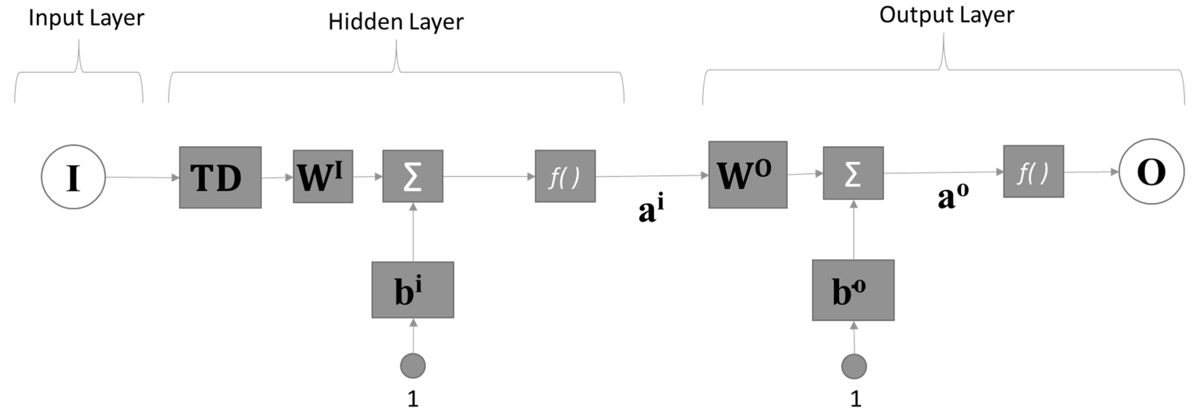
3. Artificial Neural Networks (ANNs)

Artificial NNs are used to generalize the nervous system of a human being into one or more mathematical models. The concept of ANN analysis was discovered about five decades ago, but, in the past several years, its applications have become wider and more popular due to significant advancement in technology in order to solve challenging problems regarding the faster processing speed and higher computing capacity [8,9,15,16].
Figure 4 illustrates an example of the dynamic neural network with only one time delay structure, which contains an input layer as the independent variable vector, one hidden layer of neurons with a time delay, weight and bias matrices, and an output layer as the one output neuron.
Each neuron is connected to all of the other neurons of the previous layer through a weight function w and its response vectors a i and a o are generated by the activation function f( ). The number of neurons can vary for each layer independently. The neurons in the subsequent layers receive a neuron response from the previous layer as their input. Figure 4 shows a model that has input, I, which includes five input variables of current, anode and cathode inlet flow rates, pressure, and temperature, while the output layer of the output vector, O, is the output variable. This arrangement of the ANN model allows it to perform summation and apply activation functions to determine the values of a hidden or output layer for one time step ahead. The activation function of the output layer is chosen as the linear function, while the activation functions of the hidden layer are the log-sigmoid function.
To train and validate the models, the experimental data were obtained from a fuel cell test station at. The key input variables were the current, anode and cathode inlet flow rates, anode pressure, and cathode temperature, while the key outputs measured for the performance prediction were the stack temperature in °C and the stack voltage in V.
For training, the input data were passed through the neural network to estimate the value of the output variable. When each pattern was analyzed, the network used the input data to result in an output that could be compared with the training pattern for consistency and error minimization. After the network ran through all of the input patterns, if the error was still greater than the maximum desired tolerance, the ANN model ran through all of the input patterns again, repeatedly, until all the errors met the requirements. The ANN was considered to complete the training after the ANN maintained the estimated weight and bias parameters constant, which were to be used to in the next step of validation. This next step utilized the validation data set to determine if the model was adequate. After the model was validated, the untrained input data or training data set was employed to make decisions, identify patterns, or define associations, depending on the objective of the model.
The model was achieved by minimizing the error values between the target or actual data values and the predicted data values based on the pattern given. The errors minimized in the model could be of different types, including the sum of squares error (SSE) and the mean squared error (MSE), and depend on the user preference. The SSE can be defined as
SSE = ( Z Y ) 2
where Z is the set of predicted values and Y is the set of experimental data values. The MSE can be similarly defined as
MSE = 1 n SSE
where n is the number of data points in the set [15]. These errors can then be used in different statistical analyses, including the coefficient of determination. This coefficient can be described as
R 2 = [ C o r ( Z , Y ) ] 2 = 1 SSE ( Y Y ¯ ) 2
where C o r ( Z , Y ) is the correlation coefficient, Y ¯ is the mean of the data, and ( Y Y ¯ ) 2 is the total sum of the squares. The value of R 2 varies between 0 and 1; a value of R 2 = 0.7 indicates that 70% of the total variability in the response variable is accounted for by the predictor variables, which is a satisfactory indicator for a good quality fit.
As the training speed and accuracy of the error minimization are important in order to obtain a dependable model, optimization is vital. For fast convergence, the use of Newton’s method to train ANNs is favored, but the Hessian matrix for the whole network is singular [17]. An alternative to overcome this problem is to modify the Hessian matrix, as in the Levenberg−Marquardt (LM) algorithm. The LM algorithm adds a small term µI to the Hessian matrix to improve the conditioning. Extensive research has been done for finding decent initial values for µ [18]. Small values of µ allow the performance to approach Newton’s algorithm, whereas large values of µ are identical to the gradient descent or backpropagation algorithm performance. The scaled conjugate gradient (SCG) method, created by Moller [19], is premised on conjugate directions; however, unlike other conjugate gradient algorithms, this methodology does not perform a line search at each iteration, whereas other conjugate gradient algorithms do require a line search at each iteration [19]. This increases the computational cost of the system. SCG was created to eliminate the need for the time-consuming line search. When using the scaled conjugate gradient approach, the MATLAB network training function “trainscg” updates the weight and bias values of the network while it is being trained. It can train any network as long as its weight, net input, and transfer functions all have derivative functions. It can train any network with derivative functions. The step size in the SCG method is a function of the quadratic approximation of the error function, which makes it more resilient and independent of the parameters that the user has provided for it. The step size is estimated using a different approach. The second order term is calculated as
S k ¯ = E ( ω k ¯ + σ k p k ¯ ) E ( ω ¯ k ) σ k + λ k p ¯ k
λ k is denoted as a scalar unit and changes based on the sign of σ k .
α k = μ k δ k = p j T E q ω ' ( y 1 ¯ ) ¯ p j T E ( ω ¯ ) p ¯ j ¯
where
  • ω ¯ is denoted as the vector in space R n ;
  • E ω ¯ is the global error function;
  • E ω ¯ is the gradient of error;
  • E q w ' ( y 1 ¯ ) is the quadratic approximation of error function;
  • p 1 ¯ ,   p 2 ¯ , , p k ¯ is the set of non-zero weight vectors.
  • λ k is to be updated, such that,
λ ¯ k = 2 ( λ k δ k | p k 2 | )
when
  • Δ k > 0.75 ,   then   λ k = λ k 4
  • Δ k < 0.25 ,   then   λ k =   λ k +   δ k ( 1   Δ k ) | p k 2 |
Δ k is a comparison parameter and is given by
Δ k = 2 δ k [ E ( ω k ¯ ) E ( ω ¯ k + α k p k ¯ ) ] μ k 2
A traditional neural network design replicates the operation of the human brain. The brain neurons and their connections with each other establish an equivalence relation with neural network neurons and their associated weight values (w). For a single layer with several neurons, each of the elements u j for an input vector are correlated to each neuron i with a corresponding weight w i j . There is also a bias b i connected to every neuron. This is included, basically to make the network more flexible. A scalar input is multiplied to the bias and is added to w i j u j for the vector components u j , forming the total input n i . The next input further connects to a transfer function (f).
Bayesian estimation and regularization can be traced to 1992. It requires a Hessian matrix of the objective function. For the MSE cost function and regularization by the sum of the squared weights, it follows that the Hessian matrix is a quadratic function and can be approximated using the Levenberg–Marquardt algorithm [20]. Equation (8) denotes the objective function.
F = α E w + β E D
For the Bayesian framework, weights associated to the network are seen as randomly selected variables. Equation (9) is the probability function for an array w of network weights.
f ( w D ,   α ,   β ,   M ) = f ( D w ,   β ,   M ) f ( w α , M ) f ( D α ,   β M )
M represents the neural network model utilized, while f ( w α , M ) is the prior density. f ( D w ,   β ,   M ) this is the likelihood function.

4. Results and Discussion

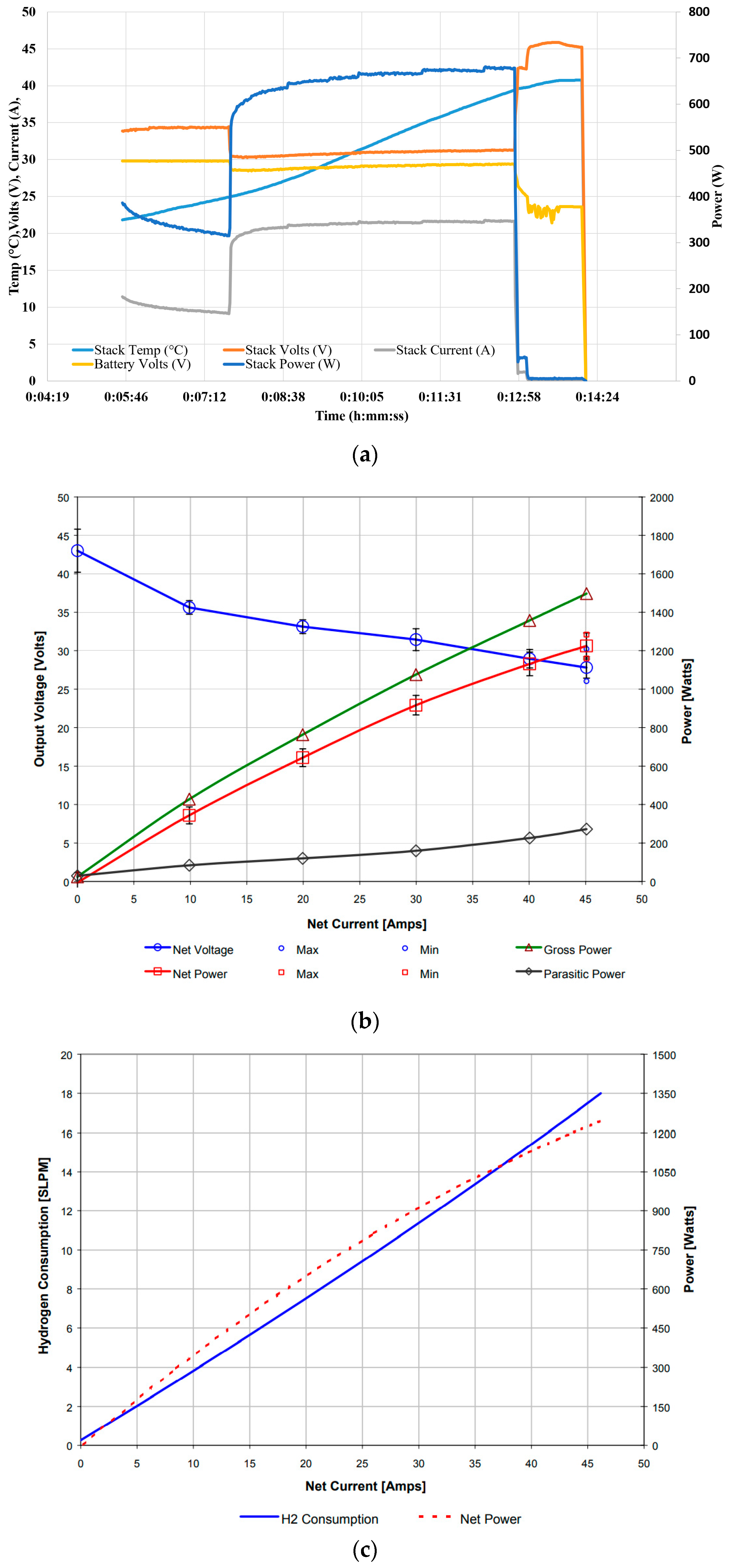
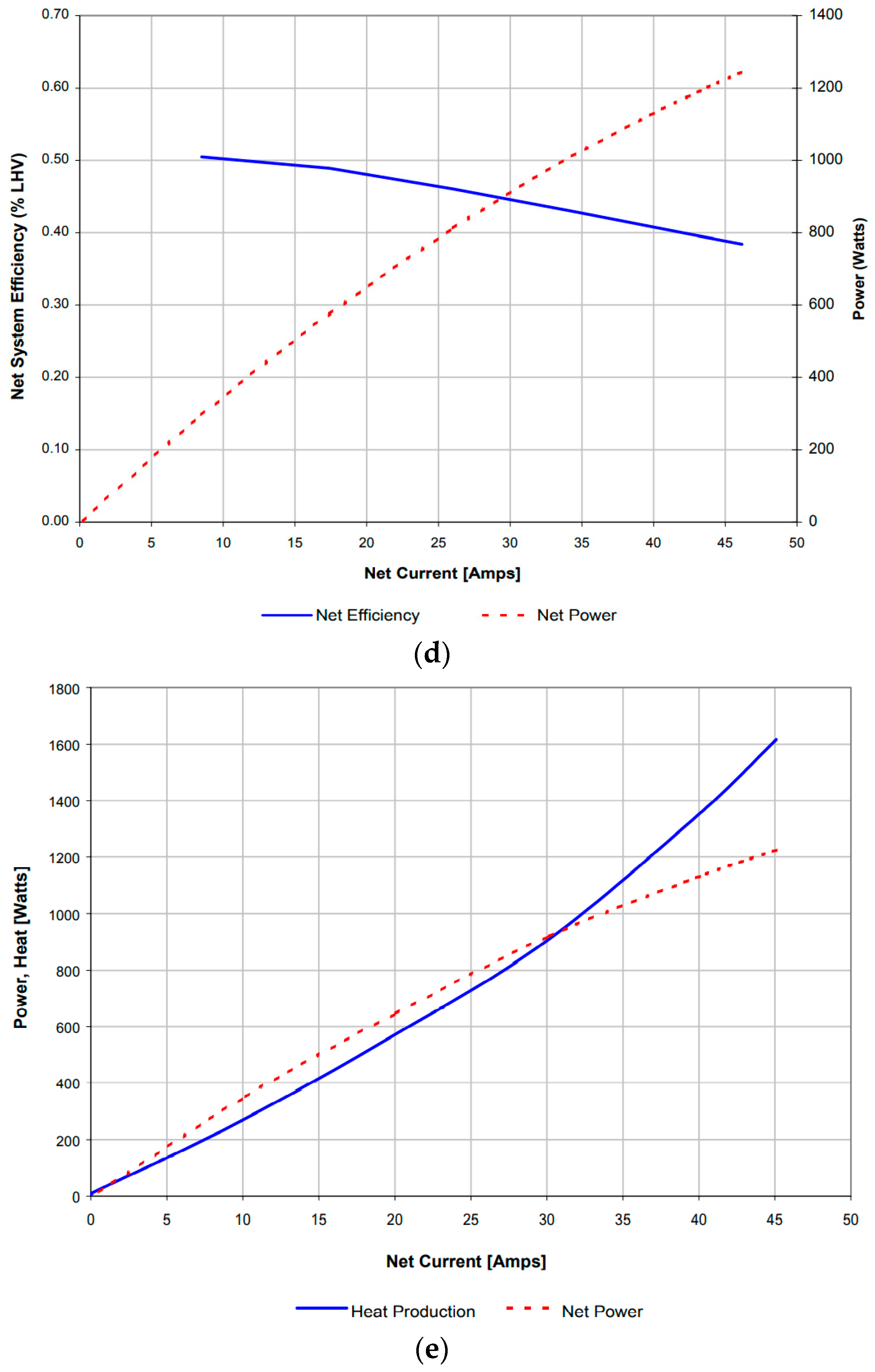
4.1. Experimental Results

Figure 5a shows the transient response characteristics of the NexaTM power module. The figure highlights the system’s response to step changes in the load. The fuel cell supplies the current to sustain the load step change. The regulator assembly supports the flow of hydrogen gas into the cell, provided there is enough fuel in the gas bottles. The changes in voltage and stack current, as well as the airflow in tandem to the step change, are captured in the figure below. In ideal conditions, the air flow rate carefully tracks the flow needed at nearly 16 slpm. After moving a load step to full power, the air pump rapidly speeds up to supply an airflow rate of nearly 85 slpm. The stack current also increases during the transient interval because of the increased parasitic power from the air compressor. A similar situation occurs after moving a load step from full power to idle. There is a decline in the airflow due to inertia in the air pump. The output voltage slowly recovers and stabilizes to 43 V over a 0.5 s interval. The net current output from Figure 5b ranges from 0–46 A. However, it can be deduced that the output voltage varies when increasing the operating load from the polarization curve. The ideal voltage for the fuel cell system was recorded as 43 VDC. The output voltage recorded at the rated power was between 26–29 VDC. Figure 5b further highlights the parasitic load with respect to the net current and output power. The system is designed in such a way that energy to support the functionality of the cooling fans, sensors, and air compressors originates from the fuel cell. When the system is idle, the power needed to support all of the components is nearly 35 watts. There is a direct correlation between the auxillary load and current, mainly to sustain higher air pump and cooling fan duties. When the fuel cell system is operating at its rated capacity, approximately 250 watts of auxiliary load is needed. As captured in Figure 5c, the rate of hydrogen consumption is also directly proportional to the rateed power. However, it can be deduced that current demand is directly correlated to hydrogen consumption. It can also be denoted that at the rated power, the highest rate of hydrogen being consumed is less than 18.5 slpm. At full power, the system efficiency from Figure 5d is 38%. The highest performance of the system is nearly 50% and this occurs at the part load. The production of waste heat from Figure 5e is also directly proportional to the output current and average net output power. Nearly 1650 W of waste heat is produced at the rated power.

4.2. ANN Results

The fitted models were obtained using MATLAB Neural Network Toolbox® software with five input variables and two output variables [13]. The models used >90% of more than 400 data points for training, and <10% for testing and validation. The number of hidden layer neurons within the single hidden layer and the type of learning algorithms were varied in the models in order to determine the best fit model. Table 2 compares the MSE and coefficient of determination of the voltage model results for the three optimization algorithms. The first column presents the type of algorithms used for the ANN modeling approach, the second column lists the selected range of hidden layer neurons that were compared, the third column shows the coefficient of determination values, and the fourth column presents the MSE of each model. Similar to Table 2, Table 3 compares the MSE and coefficient of determination of the stack temperature model results for the three algorithms. Figure 6 shows the experimental and model responses of the stack voltage where the ANN models with LM had 1, 10, and 20 hidden neurons. The y axis is the voltage in V and the x axis is the time in s. Figure 7 includes plots of the experimental and model responses of the stack voltage, where the ANN models with the Bayesian algorithm used 1, 10, and 20 hidden neurons. Figure 8 demonstrates plots of experimental and model responses of the stack voltage where the ANN models with the SCG algorithm had 1, 10, and 20 hidden neurons.
Figure 9 compares the experimental and model responses of the ANN model with LM for stack temperature. The y axis is the temperature in °C and the x axis is the time in s. Figure 10 includes the plots of the experimental and model responses of the stack temperatures, where the ANN models with using the Bayesian algorithm had 1, 10, and 20 hidden neurons. Figure 11 demonstrates the experimental and model responses of the stack temperature using an ANN with the SCG algorithm.

4.3. Discussion

Table 2 shows that most of the models resulted in a high coefficient of determination (>0.9) with a relatively low MSE. Furthermore, the model using ANN with the LM algorithm and 20 hidden neurons provided the best fit with the experimental data. The model had a coefficient determination of 0.93 and MSE of 3.478 V for the 1.2 kW PEMFC stack. Figure 6, Figure 7 and Figure 8 illustrate the same observation of the models mostly fitting well, including the models using ANNs with LM and Bayesian regularization algorithms. The models (LM and Bayesian) were able to track the data from an initial stack voltage to a drop in stack voltage for an initial steady state current load value, to a high current load at around 120s. This quick change in current resulted in an undershoot of the voltage for a few seconds before it reached the new steady state value. However, the voltage models had a slightly poorer performance when the current load was brought down to zero at around 430 s compared with the previous time frames, but were still reasonably well-matched with the empirical data. Because of this decrease in current load, the PEMFC stack voltage was observed to increase with slight overshoots.
Similarly, Table 3 shows that virtually all models consistently had very high coefficients of determination (>0.94) with a low MSE. Yet again, the model using an ANN with the LM algorithm and 20 hidden neurons provided the best fit, along with 15 hidden neurons. For the PEMFC stack, the models using an ANN with the LM algorithm had 15 and 20 hidden neurons were found to have coefficients of determination of 0.966 and 0.964, respectively, and MSEs of 2.8 and 2.9 °C, respectively. Figure 9, Figure 10 and Figure 11 illustrate how the models had similar results, including the models using ANNs with LM and Bayesian regularization algorithms. The models (LM and Bayesian) did follow the upward trend of the temperature as the stack operation continued. The temperature increased as more heat was released due to the electrochemical reaction from the PEMFC, thus bringing it to a more optimally efficient operating condition. The model results in Figure 9 and Figure 10 are virtually indistinguishable from the experimental temperature data of the PEMFC stack for nearly the entire duration of the stack operation until around 470 s to the end of the plot where an offset can be observed. This could be attributed to the relatively rapid decline of the current load down to zero, where the temperature drop was predicted to be faster than the empirical testing data.
From all of the tables and figures, it can be seen that most models for a different number of hidden neurons with the LM and Bayesian regularization algorithms could effectively approximate the PEMFC temperature data. However, the LM algorithm performed better based on the MSE and coefficient of determination, which was observed with the response plots in Figure 6 and Figure 9. Moreover, 1 to 5 neurons in the hidden layer usually resulted in a poor model accuracy compared with the higher number of neurons in the same hidden layer. Overall, the results obtained from the models presented in this paper were comparable to the results of the limited data and studies found in the literature [10,11,12,13].

5. Conclusions

The study compared the application of ANN modeling with different algorithms and hidden neurons on a PEMFC system. The models matched well to the experimental data for several varying sets of hidden neurons. Although most ANN model responses had high coefficients of determination (greater than 0.9), the ANN model using the LM algorithm showed the best fit. Thus, it can be concluded that the dynamic ANN with the LM algorithm has the best performance when implementation of such models are made in optimization of relevant control strategies. Moreover, most of these modeling approaches can be very useful tools in system optimization and control design for such an electrochemical system to improve the efficiency and stabilize the operation regardless of the transient operating conditions.

Author Contributions

Conceptualization, T.W., M.B. and A.O.; methodology T.W. and M.B.; software, M.B. and A.O.; validation, T.W., M.B. and A.O.; formal analysis, T.W. and M.B.; investigation, T.W., M.B. and A.O.; resources, A.O; data curation, T.W.; writing—original draft preparation, T.W., M.B. and A.O.; writing—review and editing, T.W., M.B. and A.O.; visualization, T.W., M.B. and A.O.; supervision, T.W., M.B. and A.O.; project administration, T.W., M.B. and A.O.; funding acquisition, T.W., M.B. and A.O. All authors have read and agreed to the published version of the manuscript.

Funding

This research received no external funding.

Data Availability Statement

Data can only be made available on request.

Conflicts of Interest

The authors declare no conflict of interest.

References

  1. Biswas, M.A.R.; Robinson, M.D. Prediction of Direct Methanol Fuel Cell Stack Performance Using Artificial Neural Network. ASME J. Electrochem. Energy Convers. Storage 2017, 14, 031008. [Google Scholar] [CrossRef]
  2. Biswas, M.; Mudiraj, S.; Lear, W.; Crisalle, O. Systematic Approach for Modeling Methanol Mass Transport on the Anode Side of Direct Methanol Fuel Cells. Int. J. Hydrogen Energy 2014, 39, 8009–8025. [Google Scholar]
  3. Mudiraj, S.; Crisalle, O.D.; Biswas, M.; Lear, W. Comprehensive Mass Transport Modeling Technique for the Cathode Side of an Open-Cathode Direct Methanol Fuel Cell. Int. J. Hydrogen Energy 2015, 40, 8137–8159. [Google Scholar]
  4. Ogungbemi, E.; Ijaodola, O.; Khatib, F.N.; Wilberforce, T.; El Hassan, Z.; Thompson, J.; Ramadan, M.; Olabi, A.G. Fuel cell membranes—Pros and cons. Energy 2019, 172, 155–172. [Google Scholar] [CrossRef] [Green Version]
  5. Ogungbemi, E.; Wilberforce, T.; Ijaodola, O.; Thompson, J.; Olabi, A.G. Review of operating condition, design parameters and material properties for proton exchange membrane fuel cells. Int. J. Energy Res. 2020, 45, 1227–1245. [Google Scholar] [CrossRef]
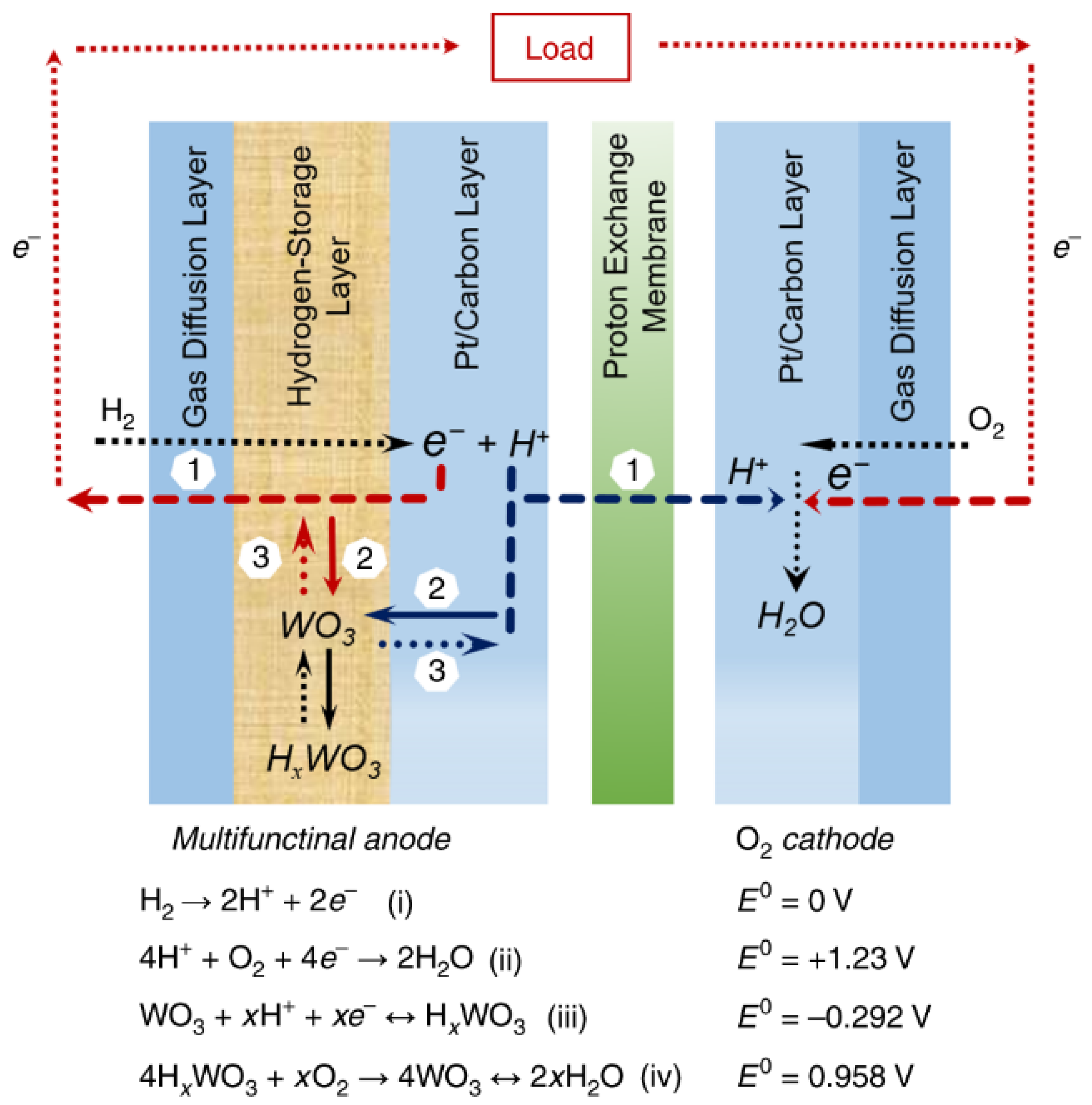
  6. Shen, G.; Liu, J.; Wu, H.B.; Xu, P.; Liu, F.; Tongsh, C.; Jiao, K.; Li, J.; Liu, M.; Cai, M.; et al. Multi-functional anodes boost the transient power and durability of proton exchange membrane fuel cells. Nat. Commun. 2020, 11, 1191. [Google Scholar] [CrossRef] [Green Version]
  7. Jayakumar, A.; Chalmers, A.; Lie, T.T. Review of prospects for adoption of fuel cell electric vehicles in New Zealand. IET Electr. Syst. Transp. 2017, 7, 259–266. [Google Scholar] [CrossRef]
  8. Miao, Q.; Cao, G.; Zhu, X. Performance analysis and fuzzy neural networks modeling of direct methanol fuel cell. J. Shanghai Univ. 2007, 11, 84–87. [Google Scholar]
  9. Biswas, M.A.R.; Robinson, M.D.; Fumo, N. Prediction of residential building energy consumption: A neural network approach. Energy 2016, 117, 84–92. [Google Scholar]
  10. Xu, L.; Xiao, J. Dynamic Modeling and Simulation of PEM Fuel Cells Based on BP Neural Network. In Proceedings of the 2011 3rd International Workshop on Intelligent Systems and Applications, Wuhan, China, 28–29 May 2011; pp. 1–3. [Google Scholar]
  11. Lopes, F.C.; Watanabe, E.H.; Rolim, L.G.B. Analysis of the time-varying behavior of a pem fuel cell stack and dynamical modeling by recurrent neural networks. In Proceedings of the Brazilian Power Electronics Conference (COBEP 2013), Gramado, Brazil, 27–31 October 2013. [Google Scholar]
  12. Li, P.; Chen, J.; Cai, T.; Liu, G. On-line identification of fuel cell model with variable neural network. In Proceedings of the 29th Chinese Control Conference, Beijing, China, 29–31 July 2010; IEEE: Piscataway, NJ, USA, 2010; pp. 1417–1421. [Google Scholar]
  13. Puranik, S.V.; Keyhani, A.; Khorrami, F. Neural Network Modeling of Proton Exchange Membrane Fuel Cell. IEEE Trans. Energy Convers. 2010, 25, 474–483. [Google Scholar] [CrossRef]
  14. Brunetto, C.; Moschetto, A.; Tina, G. PEM fuel cell testing by electrochemical impedance spectroscopy. Electr. Power Syst. Res. 2009, 79, 17–26. [Google Scholar]
  15. Hagan, M.T.; Demuth, H.B.; Beale, M.H. Neural Network Design; PWS Publishing Company: Boston, MA, USA, 1996. [Google Scholar]
  16. Robinson, M.D.; Manry, M.T. Two-Stage Second Order Training in Feedforward Neural Networks. In Proceedings of the Twenty-Sixth International FLAIRS Conference, St. Pete Beach, FL, USA, 22–24 May 2013. [Google Scholar]
  17. Wille, J. On the structure of the Hessian matrix in feedforward networks and second derivative methods. In Proceedings of the International Conference on Neural Networks, Houston, TX, USA, 12 June 1997. [Google Scholar]
  18. Dennis, J.E., Jr.; Schnabel, R.B. Numerical Methods for Unconstrained Optimization and Nonlinear Equations; Society for Industrial and Applied Mathematics: Philadelphia, PA, USA, 1996. [Google Scholar]
  19. Møller, M.F. A scaled conjugate gradient algorithm for fast supervised learning. Neural Netw. 1993, 6, 525–533. [Google Scholar] [CrossRef]
  20. Gill, P.; Murray, W. Algorithms for the solution of the nonlinear least-squares problem. SIAM J. Numer. Anal. 1978, 15, 977–992. [Google Scholar]
Figure 1. Operating characteristics for proton-exchange membrane fuel cells [6].
Energies 15 05587 g001
Figure 2. Diagram of the 1.2 kW Ballard fuel cell used for the investigation.
Energies 15 05587 g002
Figure 3. (a) Fuel cell experimental setup. (b) Wiring schematic of the load cell.
Energies 15 05587 g003
Figure 4. Neural network model example with an input layer, one hidden layer with a time delay, and an output layer.
Energies 15 05587 g004
Figure 5. (a) Fuel cell response with respect to time. (b) Polarization and power curves for the 1.2 kW Nexa fuel cell. (c) Rate of hydrogen consumption. (d) Efficiency of the system. (e) Waste heat produced from the module.
Energies 15 05587 g005aEnergies 15 05587 g005b
Figure 6. Experimental and model responses of the stack voltage using an ANN with the LM algorithm.
Energies 15 05587 g006
Figure 7. Experimental and model responses of the stack voltage using an ANN with the Bayesian-based algorithm.
Energies 15 05587 g007
Figure 8. Experimental and model responses of the stack voltage using an ANN with the SCG algorithm.
Energies 15 05587 g008
Figure 9. Experimental and model responses of the stack temperature using an ANN with the LM algorithm.
Energies 15 05587 g009
Figure 10. Experimental and model responses of the stack temperature using an ANN with the Bayesian-based algorithm.
Energies 15 05587 g010
Figure 11. Experimental and model responses of the stack temperature using an ANN with the SCG algorithm.
Energies 15 05587 g011
Table 1. Various components used.
Part NumberItem NameFunction in Setup
1Batteries2 × 12 V batteries are connected in series. The batteries power the entire system during start up, as the auxiliary unit requires 5 W prior to NexaTM completing its start up process and running normally.
2FuseEnsures the current via the circuit are below the threshold of the wires, as well as protecting the batteries and essential safety components
3ResistorDespite the desired resistances being low, the output power of the fuel cell was high; hence, a resistor to sustain the load was required. As a result, wire wound panel mount resistors with a ceramic core were selected.
4Load bank coverA cover was required as excess heat produced could cause body harm to the operator of the test rig.
5DC/DC converterThe output power from the fuel cell is direct current that is not stable. The The DC/DC converter stabilizes the DC output at 24 V. It is able to elevate the voltage level from low to high and vice versa.
6ISLE Display UnitSupports when taking readings in terms of the operational characteristics of the fuel cell.
7Isolator SwitchSupports the withdrawal of the batteries once the fuel cell is operating beyond its maximum parasitic load.
8RelayConnects the major test rig circuit with the batteries, which are independently connected in series. They are needed until the fuel cell starts operating after starting up.
9Terminal blocks/BusbarThis device allows all the resistors to be connected to either the DC/DC converter or to the relay. Every output configuration from the switch box is connected to one of the two busbars.
10Hydrogen snifferSupports the detection of potential hydrogen leakage.
11Fuel/Hydrogen cylinderServes as a storage unit for the investigation.
12Fuel regulatorFor the monitoring of hydrogen in the cylinder. It also aid in regulating the output pressure from the fuel cell.
13PC/Data logging softwareNexamonOEM data logging software supports the reading and recording of data based on the experimental setup.
14Hydrogen housing unitsTo ensure the hydrogen gas bottle is held in position during the experiment, a housing unit is required.
15Cylinder bracketsIts also protects the gas bottle during the experiment
16Power supplyThe test rig was powered using energy from the grid with the aid of extension cables.
17Switch boxesHouses the switches.
18Water collection unitThe water produced as by product from the operation of the fuel cell is carefully delivered to a tank, where the product water can be measured.
19Ballard fuel cell1.2 kW PEMFC to be analysed via dynamic loading.
Table 2. Statistical analysis of the model results for the stack voltage.
ANN Learning AlgorithmsNumber of Hidden NeuronsCoefficient of DeterminationMean Squared Error (V)
LM10.9164.150
LM50.9193.998
LM100.9233.790
LM150.9233.842
LM200.9303.478
SCG10.9134.319
SCG50.9014.874
SCG100.8119.691
SCG150.9054.706
SCG200.8806.507
Bayesian10.9174.093
Bayesian50.9174.093
Bayesian100.9174.091
Bayesian150.9174.091
Bayesian200.9174.090
Table 3. Statistical analysis of the model results for the stack temperature.
ANN StructureNumber of
Hidden Neurons
Coefficient of
Determination
Mean Squared Error (°C)
LM10.9613.131
LM50.9613.121
LM100.9613.141
LM150.9662.761
LM200.9642.922
SCG10.9523.807
SCG50.9414.861
SCG100.9593.306
SCG150.9593.312
SCG200.9424.665
Bayesian10.9613.126
Bayesian50.9613.121
Bayesian100.9613.122
Bayesian150.9613.122
Bayesian200.9613.121
Publisher’s Note: MDPI stays neutral with regard to jurisdictional claims in published maps and institutional affiliations.

