Numerical Modelling of the Effects of Liquefaction on the Upheaval Buckling of Offshore Pipelines Using the PM4Sand Model

Abstract

The buckling tendency of an offshore pipeline buried in a liquefiable soil aggravates under earthquake situations. Moreover, to understand the upheaval displacement behavior of an offshore pipeline under dynamic loading, it is crucial to understand the variation of liquefaction potential within the soil bed. Thus, in the present study, the variation of the liquefaction potential within the soil body and its effect on the pipeline upheaval displacement (u) and post-shake uplift resistance (V_up) is investigated using a finite element package called PLAXIS 2D. The study was performed for different seismic and soil conditions. To define the soil, two advanced constitutive models are used. The static stages are modelled with the ‘Hardening Soil Model with small strain’ (HSS model), while the dynamic stage is modelled with the PM4Sand model. Moreover, the problem is defined as a 2d plane strain problem. The pipe is considered to be covered with Nevada sand. Several parameters such as a sand-density index (D_r), pipe embedment depth (H), seismic frequency (f) and amplitude are varied to study the variation of the soil liquefaction potential, the pipe upheaval buckling and the post-shake uplift resistance. The model is validated with past studies and a considerable match is obtained. The liquefaction potential is shown using the shadings of a user-defined parameter called a pore water pressure ratio (r_u). Moreover, the variation of pipe upheaval displacement (u) and pipe uplift resistance (V_up) are shown using various plots. Thus, it is observed that the liquefaction potential is reduced with an increase in the frequency and the amplitude of the seismic signal. Moreover, the peak upheaval buckling, and the duration of earthquake loading to reach the peak upheaval buckling, decreased with an increase in the earthquake signal frequency. Again, the variation of post-peak uplift resistance of the buried pipeline with the pipe embedment depth is observed to be independent of the signal parameters. However, the variation of uplift resistance of the pipeline with the soil relative density is influenced by the signal parameters.

1. Introduction

Offshore pipelines are key components of marine gas and oil exploitation systems. They are mostly used to carry processed and unprocessed oils, cables, lubricants and water. For this reason, they are also called the lifeline systems for offshore petroleum extraction facilities. Offshore pipelines carrying unprocessed oil are often subjected to longitudinal thermal compressive stress, which makes them susceptible to thermal buckling. Upheaval thermal buckling is very common for buried pipelines [1,2,3]. Furthermore, the buckling of the pipeline is amplified when seismic events are considered. Seismic events such as the 1994 Northridge earthquake [4] or the 1999 Chi-Chi earthquake [5] had disastrous effects on the pipeline system, and even caused the failure of several large diameter pipelines. The failure of pipelines has various irreversible and widespread consequences on the environment, as well as on human lives. At the same time, repairing and recommissioning pipelines can incur huge expenditures. Thus, to avoid these issues, further research needs to address the effect of earthquakes on offshore pipeline systems.

The study of thermal buckling of pipelines under static conditions started with the study of the uplift of anchors [6,7]. Later, extensive numerical [2,8,9], analytical [10] and experimental studies [11,12,13] were performed. Some researchers proposed upper limits for the uplift capacity [14], while others proposed methodologies to predict the uplift capacity of a pipeline [1,15]. Several studies explored the stress-strain behavior of pipelines during buckling, and the parameters affecting the stress-strain behavior [12,16,17]. The displacement pattern of the soil around the pipeline was studied by other researchers [18,19]. The major parameters affecting the stress-strain behavior, uplift capacity and failure mechanism are observed to be the pipe diameter, the embedment depth, the soil unit weight, the pipe surface roughness, the interface tensile capacity and the existence of initial imperfections. Researchers observed an increase in the uplift capacity when increasing the pipe embedment depth and the soil density for cohesive [1,8,15] and cohesionless soils [20,21,22]. Newson and Deljoui [8] numerically explored the undrained uplift capacity of a buried pipeline, and found that the undrained uplift capacity increased with increasing embedment depth until a peak value was reached. Moreover, Maitra et al. [1] analytically proposed a methodology to calculate the uplift capacity factor of a buried pipeline using pipe embedment depth, soil unit weight and pipe-soil interface properties. Several full-scale experimental studies were performed by Schaminee et al. [15] using a wide variety of soil types to explore the load-displacement behavior of a buried pipeline under a vertical and axial loading. They [15] also proposed an expression to calculate the pipeline uplift capacity from an embedment depth ratio and the soil unit weight. Furthermore, the failure mechanism of the soil around the pipeline due to pipe uplift was also observed to change from global to a local shear failure mechanism with an increase in the pipe embedment depth and the soil density [1,2,23]. Seth et al. [3] numerically studied the failure mechanism patterns and found that the failure mechanism is changed from a global to local mode beyond a limiting embedment depth. Cheuk et al. [23] conducted several scaled model tests and demonstrated the deformation of different soil layers above the pipeline and soil failure mechanism using the particle image velocimetry (PIV) technique. The effect of the shear and tensile capacity of the pipe’s outer surface on the uplift behavior of a pipeline was also studied by authors such as Maitra et al. [1], Seth et al. [2,18], Cheuk et al. [24], and Kumar et al. [25]. Maitra et al. [1] found that the peak uplift capacity was changed from 9.2 to 12, when the pipeline’s outer surface was changed from perfectly smooth to rough. Similarly, Kumar et al. [25] observed that the limiting embedment depth corresponding to the change in failure mode was decreased when the pipe-soil interface tensile capacity was changed from zero to infinity. Moreover, the uplift capacity was observed to be reduced with initial imperfections in the pipelines [16,26]. Several theoretical models are also proposed to study the upheaval buckling behavior of the pipeline [27].

Earthquake events can cause buckling of a pipeline in two ways: (a) by liquefaction of the surrounding soil, and (b) with the movement of the soil mass at a fault. In the presence of loose saturated soil, liquefaction may occur under seismic loading, which may further give rise to the floatation or the upheaval buckling of the pipeline [28,29,30,31,32,33,34,35]. Given these issues, the liquefaction phenomenon around an offshore pipeline has also been addressed in previous research. Several researchers numerically and experimentally studied the generation of excess pore water pressure around an offshore pipeline, which further lead to the liquefaction of the soil mass [28,31,36,37]. Ling et al. [28] used the Pastor-Zienkiewicz Mark-III constitutive model to define the soil and numerically studied the ground response in terms of acceleration, excess pore water pressure, earth pressure and pipeline upheaval buckling under a synthetic seismic loading. Furthermore, Maotian et al. [31] performed a parametric study using the finite element method to study the effect of several soil parameters such as the deformation modulus, the Poisson ratio, and the permeability coefficient of the soil on the liquefaction potential of the soil around a pipeline under seismic loading. They observed that with the decrease in the deformation modulus, the permeability coefficient, and the Poisson’s ratio, the excess pore water pressure and, in turn, the liquefaction potential of the soil decreased. Some analytical models have also been proposed to predict the liquefaction potential around an offshore pipeline [35,37]. These models primarily considered soil and pipe parameters such as the soil hydraulic conductivity, the unit weight, the Poisson ratio, the deformation modulus, and the pipe diameter to generate the prediction models.

Several authors studied the direct influence of different soil parameters on the liquefaction-induced pipe upheaval buckling [29,33,34,38]. Huang et al. [33] referred that the buoyancy force applied to the pipeline by the surrounding liquefied soil is the primary reason behind the pipeline upheaval buckling. Furthermore, the effect of soil parameters such as the soil dilatancy angle, friction angle and density ratio on the pipe upheaval buckling were studied by several authors, and it was observed that these parameters have a major role on the behavior of the buoyancy force that facilitates pipeline upheaval buckling [29,39]. Moreover, the effects of some other parameters, such as the pipe diameter and burial depth, water table and thickness of the saturated soil layer on the upheaval floatation of pipelines were explored by Saeedzadeh and Hataf [29] and Chian and Madubhushi [38]. It was observed that the upheaval buckling of a pipeline is directly proportional to the pipe diameter and the depth of the water table. In contrast, the pipeline upheaval displacement is inversely proportional to the distance from the source of vibration.

It is observed that experimental, numerical and theoretical studies are crucial for understanding the mechanism of pipeline upheaval displacement in liquefied soil. However, in previous studies, the floatation of the pipeline is described from observations of pore water pressure at the surrounding area of the pipeline only. Conversely, the variation of pore water pressure throughout the soil bed was very difficult to obtain. The lack of knowledge of the variation of liquefaction potential throughout the soil-bed restricted researchers from fully understanding the upheaval buckling behavior of pipes in earthquake and post-earthquake soil conditions. Thus, there is a pressing need for further studies in order to better understand the pipeline upheaval buckling at earthquake and post-earthquake stages. The recent development of some advanced constitutive models such as the PM4Sand model have enabled researchers to visualize the variation of liquefaction potential throughout the soil bed, which further enables a more detailed study of the pipeline buckling behavior under a dynamic loading condition.

The present article presents an innovative, extensive study that has been performed on the buckling behavior of offshore pipelines under static and dynamic conditions. The PM4Sand model is used to predict the variation in liquefaction potential within the soil bed. It is also used to help describe the effects of earthquake signals and soil parameters on the floatation or upheaval displacement of a pipeline in liquefiable soil, through the changes in the liquefaction potential within the soil bed under dynamic loading. At the same time, the drained uplift resistance of a pipeline at a post-earthquake/post-shake condition is also explored.

In the current study, several numerical analyses are performed using the finite element software PLAXIS 2D 2019 [40] to explore the liquefaction potential of a soil, the upheaval buckling of a pipeline under earthquake loading and the drained uplift resistance of the soil around the pipeline in the post-earthquake stage. Moreover, a parametric study is performed by varying different soil and seismic signal parameters. In this study, Nevada sand is used as a backfill material, and three densities (D_r) are considered to observe the upheaval buckling and uplift capacity variation. Moreover, the amplitude (a) and frequency (f) of the dynamic loading and the pipe embedment depth (H) are also varied. A sinusoidal signal is used to simulate the earthquake event [34]. A synthetic earthquake signal is used instead of a natural earthquake, so that the frequency and amplitude of the seismic signal can be varied systematically. Subsequently, the liquefaction potential of the soil mass under seismic loading is visualized using a user-defined parameter pore water pressure ratio (r_u), which is defined later. The soil is considered to be completely liquefied if the value of r_u reaches or exceeds 1. Moreover, the upheaval buckling of the pipeline under the dynamic loading is considered to be the upheaval buckling of the pipeline after the end of the simulated earthquake. Finally, in the post-earthquake stage, the uplift resistance of the pipeline is calculated using the double-tangent method from the load-displacement curve, similar to what was used by Seth et al. [2] and Kumar et al. [25]. The variation of the pipeline upheaval buckling and post-shake uplift resistance of the soil as a function of the variation of the seismic, soil and pipeline parameters is then discussed using several plots.

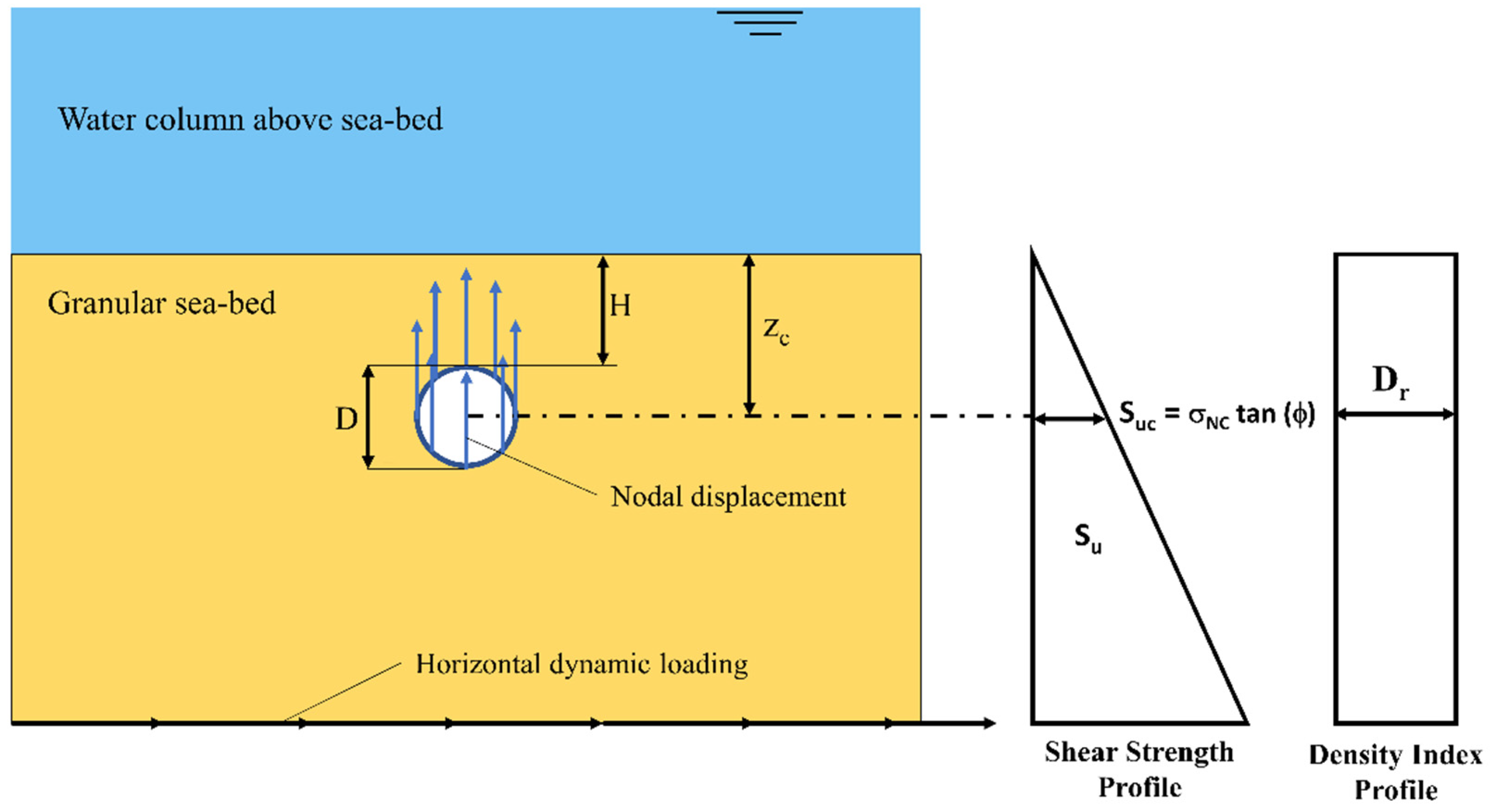
2. Problem Statement

An offshore pipeline with diameter D is buried at a depth of H within a granular seabed. The seabed is considered to be constituted by Nevada sand. The effect of the earthquake loading on the upheaval buckling behavior of the pipeline is explored in this study. The upheaval buckling behavior of the pipeline is studied in two stages, namely the earthquake stage and the post-earthquake stage. In the earthquake stage, the upheaval buckling or floatation of the pipeline under seismic loading is studied. In the post-earthquake stage, the drained uplift resistance (under thermal buckling) of the soil on the pipeline is investigated. The degree of liquefaction of the soil under various seismic signals and soil densities is also studied. Only the horizontal seismic component is considered in the current study. Thus, the seismic event is simulated in the earthquake stage by applying a horizontal sinusoidal signal at the bottom of the soil volume. In the post-earthquake stage, nodal displacements are applied to the pipeline to simulate the thermal buckling mechanism.

A schematic diagram of the pipeline is shown in Figure 1. The diameter of the pipeline is represented by D, and the embedment depth is represented by H. The shear strength of the soil varies with depth. Moreover, the shear strength at the center level of the pipeline is considered to calculate its uplift capacity. The distance of the center of the pipeline from the top of the seabed is Z_c, which is used to calculate the effective shear stress. The relative density of the soil is considered to be constant (D_r) throughout the depth of the soil. The upward nodal displacement applied to the pipeline is shown using upward arrows, while the horizontal seismic displacements are represented as the horizontal arrows at the bottom of the soil mass. The water table is above the soil and is represented by the sky-blue block. Moreover, there are several assumptions which are listed below:

• The soil is considered to be submerged.
• The outer surface of the pipeline is considered to be completely rough. Thus, the full friction angle of the soil is mobilized at the pipe–soil interface.
• The pipe–soil interface is considered to have negligible tensile capacity, and the soil does not remain connected to the pipe bottom during the pipe upheaval buckling.
• The pipeline is subjected to hydrostatic pressure from the outside, as it is buried within a submerged seabed. However, the inside of the pipeline is considered dry, and no internal pressure is considered in the current study.
• The stiffness of the pipeline is considered to be very high to prevent a change in the shape of the pipe cross-section under hydrostatic and soil pressure.
• The effect of the hydrodynamic wave loading is neglected in the post-earthquake stage.
• The problem is modelled as a 2D plain-strain problem, as the pipe-soil interaction is considered to be homogeneous throughout the pipeline length.

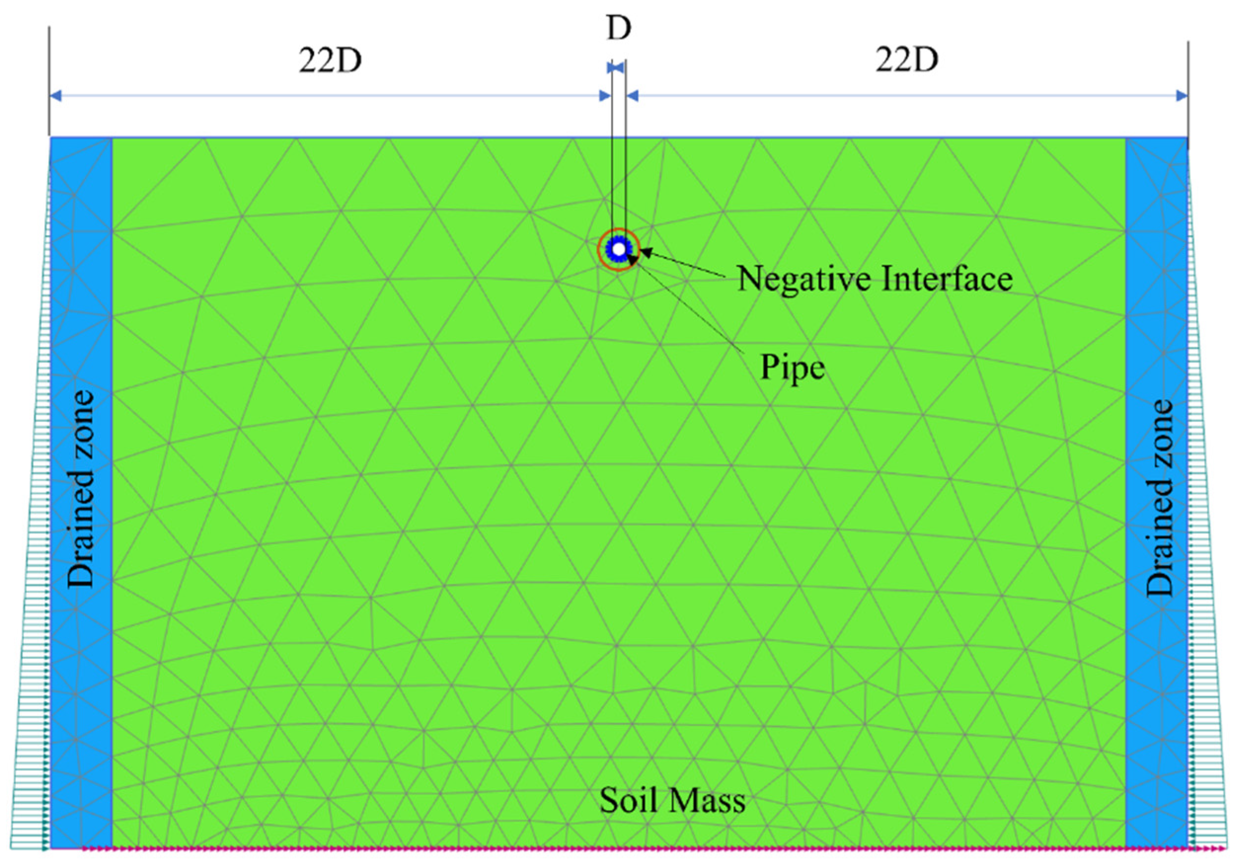
3. Numerical Modelling

An offshore pipeline has a very high slenderness ratio (i.e., length-to-diameter ratio). In addition, the deformation of the pipeline in the longitudinal direction is negligible compared to the deformation in the plane of the pipe cross-section. Thus, the pipeline and the soil are modelled as a 2D plane strain problem. The numerical study is performed in two stages using a finite element (FE) package called PLAXIS 2D. In the earthquake stage, the frequency (f) and the amplitude (a) of the dynamic loading, the embedment depth of the pipeline (H) and the density of the Nevada sand (D_r) are varied to study the liquefaction potential of the soil mass and the floatation of the pipeline. On the other hand, the uplift resistance (V_up) on the pipeline is studied for different seismic and soil parameters in the post-earthquake stage.

3.1. Boundary Dimensions, Condition and Model Discretization

Boundary optimization studies were performed under static loading to choose a suitable boundary dimension. Several trial numerical analyses with different boundary sizes were performed, and the minimum boundary dimension for which the boundary conditions did not interfere with the result (failure mechanism and uplift capacity) is considered as the required boundary dimension. Thus, in the current study, the vertical boundaries are at 22 times the pipeline diameter on each side of the pipeline. Moreover, the bottom boundary was at 24 times the pipe diameter from the bottom of the pipeline with the deepest embedment depth (H/D = 10). A boundary dimension larger than the required boundary dimension is considered to extensively study the liquefaction potential of the soil mass under seismic loading.

The deformation conditions of the boundaries are considered in such a way that the lateral displacement is restrained at the vertical boundaries, and both the lateral and vertical displacements are restrained at the bottom boundary. Moreover, as a dynamic boundary condition, a ‘tied degrees of freedom’ boundary condition is used at the vertical boundaries, and a ‘compliant base’ boundary condition is applied at the bottom boundary. The tied degrees of freedom condition connect the nodes of the same elevation at the vertical boundaries to facilitate the one-dimensional wave propagation, while the compliant base condition is used to ensure the absorbance of the reflected wave from the above layers [41]. Such dynamic boundary conditions create an absorbent boundary around the soil mass and have been used extensively by past researchers [25]. Furthermore, two additional drained soil layers were also added on the two sides of the soil volume to avoid stress concentration during the dynamic analysis with the tied degrees of freedom and the compliant base boundary conditions [42]. As referred to previously, the water table is considered to be at the top of the soil mass, thus making the soil mass submerged.

After defining the boundary conditions and the dimensions, the material properties and constitutive models for the soil and the structure are chosen. Afterwards, the entire soil volume is discretized into a number of elements to define the finite element mesh. Two elements are available in PLAXIS 2D to model a soil volume, namely 6-node and 15-node triangular elements. In the current study, the 15-node triangular element is used to model the soil for better accuracy. At the same time, 5-node beam elements are used to model the pipeline cross-section. The relative element size of the mesh is considered as 1.33. Thus, the whole soil volume is discretized into 687 elements and 6102 nodes. The mesh size used in this study is decided by a mess optimization study with a different mesh size. It is observed that the current mesh size (relative element size 1.33) caused very little sacrifice to the accuracy of the result, while reducing the computational cost to a considerable extent. A typical discretized soil volume is shown in Figure 2.

3.2. Material Modelling

The soil is modelled using two different constitutive models in PLAXIS 2D. The dynamic analysis was modelled by the advanced constitutive model PM4Sand [39], which has been used in previous research to simulate the effects of liquefaction [43,44,45]. However, the static phases are modelled using the HS small (HSS) model [40], due to the inability of the PM4Sand model to accurately calculate the static loading conditions. In a particular stage, stress states and displacements of a soil volume are calculated as per the defined stiffness and strength parameters of the materials in that stage. However, at the beginning of each stage, the internal variables are initialized as per the stress state of the previous stage. For example, the internal variables in the earthquake stage are initialized as per the calculation of the installation stage, and the change in the material model and stiffness and strength parameters have a negligible effect on the results [41]. The mesh size and the element types are kept the same at all the stages of analysis, i.e., 15-node triangular elements for the soil volume, and 5-node beam elements for the pipe cross-section with a relative element size of 1.33. The seabed is considered submerged and is made of Nevada sand. The properties considered for the Nevada sand are based on past studies [29,39]. To study the effect of the density of the soil on the upheaval buckling behavior of the pipeline, a range of soil density indices were considered, namely 40%, 50% and 60%. Given that an earthquake is a phenomenon with a very short duration, the pore water pressure cannot dissipate during this event, thus resulting in an undrained condition. On the other hand, the pipe buckling occurs comparatively at a slower rate and gives rise to a drained condition. Thus, the earthquake stage is analyzed in undrained conditions, while during the static case, the upheaval buckling of the pipeline is analyzed in drained conditions. Furthermore, the post-shake uplift resistance on the pipeline is calculated from the load–displacement curve using the double tangent method [2,25].

Two sets of parameters are defined for two different models used for the analysis. The maximum and minimum void ratios are considered as 0.847 and 0.517, respectively. From these values, the initial void ratios are calculated for the different density (D_r) of the Nevada sand. The sand is considered completely cohesionless and the range of values of the friction angle are given in

Table 1. Properties of the soil incorporated in the HSS model for the static analysis.

Parameter	Input
Density Index of Nevada sand (Dr%)	40	50	60
Initial Void ratio (einit)	0.715	0.682	0.649
Saturated unit weight of soil (γsat) (kN/m3)	19.25	19.55	19.74
$E_{50}^{ref}$ (kN/m2)	2.40 × 104	3.00 × 104	3.60 × 104
$E_{oed}^{ref}$ (kN/m2)	2.40 × 104	3.00 × 104	3.60 × 104
$E_{ur}^{ref}$ (kN/m2)	7.20 × 104	9.00 × 104	1.08 × 105
m	0.58	0.54	0.52
Friction angle (φ′) (degree)	32.5	33.9	36.4
Dilatancy angle (ψ) (degree)	1.9	3.7	4.2
$G_0^{ref}$ (Mpa)	87.2	94	100.8
γ0.7	1.60 × 10−4	1.50 × 10−4	1.40 × 10−4
Poisson ratio (ν′ur)	0.3	0.3	0.3
Pref (kN/m3)	100	100	100
Failure ratio (Rf)	0.950	0.937	0.925
Permeability of sand (Kx, Ky) (m/s)	6.82 × 10−5	6.38 × 10−5	5.55 × 10−5
Rayleigh damping α	2	2	2
Rayleigh damping β	2.70 × 10−3	2.70 × 10−3	2.70 × 10−3
Interface shear capacity (Rinter)	1	1	1
Interface tensile capacity	0	0	0

. The stiffness of the soil is represented in the HSS model using four parameters: $E_{50}^{ref}$, $E_{oed}^{ref}$, $E_{ur}^{ref}$, and m, where $E_{50}^{ref}$ is the secant stiffness from the standard drained triaxial test, $E_{oed}^{ref}$ is the tangent stiffness for the primary oedometer loading, $E_{ur}^{ref}$ is the unloading/reloading stiffness from the drained triaxial test, and m is the power for the stress-level dependency of the stiffness. Furthermore, the reference confining pressure $p^{ref}$ is set to 100 stress units (default value). Although the stiffness parameters are generally obtained experimentally, when experimental data are unavailable, these parameters can be calculated using empirical equations proposed by different researchers. For example, the value of $E_{50}^{ref}$ can be calculated using Equation (1), given by Minga and Burd [45]:

$$E_{50}^{ref}=\mathrm{60,000}\times \left(\raisebox{1ex}{$D_r$}\!\left/ \!\raisebox{-1ex}{$100$}\right.\right){\mathrm{kN}/\mathrm{m}}^2$$

(1)

Similarly, $E_{oed}^{ref}$ and $E_{ur}^{ref}$ can be determined using Equation (2):

$$E_{oed}^{ref}=E_{50}^{ref}=\left(\raisebox{1ex}{$E_{ur}^{ref}$}\!\left/ \!\raisebox{-1ex}{$3$}\right.\right)$$

(2)

Along with these parameters, the HSS model uses two additional parameters, $G_0^{ref}$ and ${\gamma }_{0.7}$, where $E_0^{ref}$ is the reference shear modulus for strains lesser than 10⁻⁶, and ${\gamma }_{0.7}$ is the threshold shear strain at which the shear modulus becomes almost 70% of the initial shear modulus. These parameters are determined using Equations (3) and (4) [39]:

$$G_0^{ref}=\mathrm{60,000}+\mathrm{68,000}\times \left(\raisebox{1ex}{$D_r$}\!\left/ \!\raisebox{-1ex}{$100$}\right.\right) \mathrm{kPa}$$

(3)

$${\gamma }_{0.7}=(2-D_r/100)\times {10}^{-4}$$

(4)

The remaining parameters are provided in Table 1.

For the PM4Sand model, several parameters are determined from the relative density of the sand and default values are considered for several parameters. The SPT value of the sand (N₁)₆₀ is back-calculated from the relative density of the sand using Equation (5). Consecutively, the shear modulus coefficient G₀ is calculated from the (N₁)₆₀ using Equation (6) [39].

$${\left(N_1\right)}_{60}=46\times {(D_r)}^2$$

(5)

$$G_0=167\sqrt{{(N_1)}_{60}+2.5}$$

(6)

Another important parameter in the PM4Sand model is the contraction rate parameter (h_p0), which adjusts the contractiveness of the model and also calibrates the cyclic resistance ratio (CRR) of the soil. The value of this parameter was obtained from the model description given by Boulanger and Ziotopoulou [39]. For the remaining parameters, the default values are considered as specified by Boulanger and Ziotopoulou [39] and are given in

Table 2. Properties of the soil incorporated in the PM4Sand model for the dynamic analysis.

Parameter	Input
Density index of Nevada sand (Dr%)	40	50	60
Initial void ratio (einit)	0.715	0.682	0.649
Saturated unit weight of soil (γsat) (kN/m3)	19.25	19.55	19.74
Corrected SPT value ((N1)60)	7	12	17
Shear modulus coefficient (G0)	514.73	635.92	737.45
Contraction rate parameter (hp0)	0.53	0.4	0.63
Atmospheric pressure (pA) (kPa)	101.3	101.3	101.3
Maximum void ratio (emax)	0.847	0.847	0.847
Minimum void ratio (emin)	0.517	0.517	0.517
Bounding surface parameter (nb)	0.5	0.5	0.5
Dilatancy surface parameter (nd)	0.1	0.1	0.1
Critical state friction angle (φcv) (degree)	33	33	33
Poisson ratio (ν)	0.3	0.3	0.3
Critical state line parameter (Q)	10	10	10
Critical state line parameter (R)	1.5	1.5	1.5
Permeability of sand (Kx, Ky) (m/s)	6.82 × 10−5	6.38 × 10−5	5.55 × 10−5
Rayleigh damping α	2	2	2
Rayleigh damping β	2.70 × 10−3	2.70 × 10−3	2.70 × 10−3
Interface shear capacity (Rinter)	1	1	1
Interface tensile capacity	0	0	0

.

Regarding the selected model for damping, Rayleigh damping coefficients of the sand medium are considered by following the specification of Ling et al. [28]. Therefore, mass (α) and stiffness (β) proportional damping coefficients of 2 and 2.7 × 10⁻³ were considered. The permeability coefficients of the soil are considered to be the same for both the models, and are given in Table 1 and Table 2.

The pipeline is considered to be a rigid pipe with a much higher flexural stiffness than the surrounding soil. The pipeline cross-section is designed as a tunnel element (which is an element available in the PLAXIS 2D library) and an elastic plate material is used to model the pipeline. Moreover, the pipe cross-section is discretized using a 5 node beam element. An interface model is also introduced at the outer surface of the pipeline to incorporate the interface properties. Generally, anticorrosive agents are applied at the outer surface of the pipeline, resulting in a rough outer surface of the pipeline. The outer surface of the pipeline is thus considered to be perfectly rough, which implies that the whole soil friction is mobilized at the pipe-soil interface and the interface shear capacity factor R_inter is set as 1 [2,22]. Moreover, the tensile capacity at the soil-pipe interface is considered to be insignificant during the pipe upheaval buckling. Thus, the interface tensile capacity of the pipe is considered to be zero for the entire analysis. The parameters used to define the pipeline are given in

Table 3. Properties of the pipeline.

Parameter	Input
Element	Pipeline
Material type	Elastic
In-plane axial stiffness (kN/m)	48 × 106
Out-of-the-plane axial stiffness (kN/m)	48 × 106
Flexural rigidity (kN·m2/m)	5.27 × 106
Diameter (D) (m)	1
Unit weight of pipeline (kN/m/m)	1
Poisson’s ratio (ν)	0.15

.

3.3. Phases of Analysis

The analysis is performed in four phases, which are discussed below:

3.3.1. Initial Phase

The initial stresses are generated in this phase using the K0-procedure and considering the stress history of the soil. This phase is modelled using the HSS constitutive model. All the structures and interfaces are deactivated in this stage.

3.3.2. Phase 1—Installation

This phase simulates the installation of the pipeline. The pipeline structure is activated in this phase. However, the loading and displacements are kept deactivated. The soil elements inside the pipeline are deactivated, and the interior of the pipeline is kept dry. The HSS model is used to define the soil in this model.

3.3.3. Phase 2—Earthquake

In this phase, the constitutive model of the soil is changed to the PM4Sand model. However, the drained zone at the two sides of the soil volume is still defined by the HSS model. The dynamic loading at the bottom of the soil volume is activated. The nodal-displacement applied to the pipeline is still deactivated. The loading condition is kept undrained in this stage.

In the earthquake phase, a dynamic loading (acceleration) is applied at the bottom of the soil mass. To study the effect of a seismic event on the pipeline upheaval buckling, a series of synthetic sinusoidal seismic waves are applied horizontally at the soil bottom. The amplitudes of the waves are 0.05 g, 0.1 g, 0.3 g and 0.5 g (g is the gravitational acceleration), and their frequencies are 1 Hz, 2 Hz 3 Hz, and 4 Hz. The earthquake loading duration is considered 30 s for all the analyses. The synthetic earthquake wave is represented by:

A = A₀ · sin(ωt)

(7)

where A is the acceleration at time t, A₀ is the amplitude and ω is the wave frequency in rad/s.

Following the earthquake phase, a nodal displacement equal to one diameter is then applied to the pipeline to study its drained post-peak uplift resistance under thermal buckling during the post-earthquake stage.

3.3.4. Phase 3—Post-Earthquake

The constitutive model defining the soil volume is changed back to the HSS model in this phase. The dynamic loading is deactivated. However, the nodal displacements of the pipeline are activated in this stage, and the upheaval buckling of the pipeline is in drained conditions.

Furthermore, in a particular stage, stress states and displacements of a soil volume are calculated as per the defined stiffness and strength parameters of that stage. However, at the beginning of each stage of calculation, the internal variables are initialized as per the stress state of the previous stage. For example, the internal variables in the earthquake stage are initialized as per the calculation of the installation stage, and the change in the material model and stiffness and strength parameters have a negligible effect on the results [44].

3.4. Validation of the Selected Soil Model

Before performing the analyses of the proposed study, a preliminary validation of the performance of the PM4Sand model was carried out using the results of the studies by Saeedzadeh and Hataf [29] and Ling et al. [28,36]. Saeedzadeh and Hataf [29] analyzed the dynamic behavior of a pipe buried in a liquefiable soil using the Hardening Soil constitutive model of the finite element software PLAXIS 2D. The analysis was performed experimentally by Ling et al. [36] and numerically by Ling et al. [1] using the Pastor–Zienkiewicz Mark-III soil model implemented in the DIANA-SWANDYNE II software. The soil was considered as a Nevada sand with a density index of 38%. The analysis involved applying a dynamic loading defined by a sinusoidal acceleration, with an amplitude of 0.6 g and a frequency of 3 Hz for 10 s. A similar analysis was performed in the current study using the PM4Sand constitutive model. The results obtained for the upheaval buckling of the pipeline under dynamic loading were then compared with the results from Saeedzadeh and Hataf [29] and Ling et al. [28,36]. The comparison between the results of the current study and the past studies are shown in Figure 3.

The comparison between the upheaval buckling of the pipeline shown in Figure 3 indicates that the pipe upheaval buckling predicted by the PM4Sand model closely matches the results obtained by Ling et al. [28] and Saeedzadeh and Hataf [29]. Even though there is some deviation in the magnitude of the results obtained from the current model and those obtained by Ling et al. [36], the prediction of the current model exhibits a trend similar to that of the results obtained by Ling et al. [36].

4. Results and Discussions

The soil behavior and pipe upheaval buckling under earthquake loading are discussed in the current section. Both the earthquake stage and the post-earthquake stages are considered in the discussion.

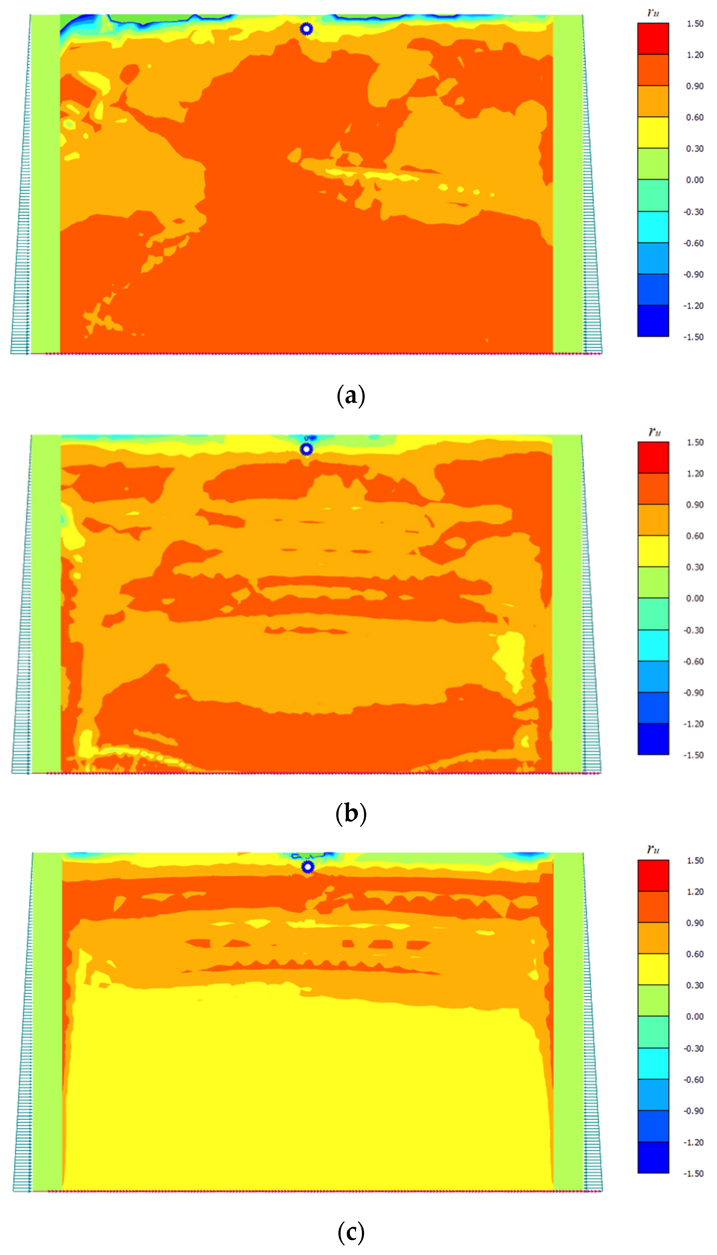
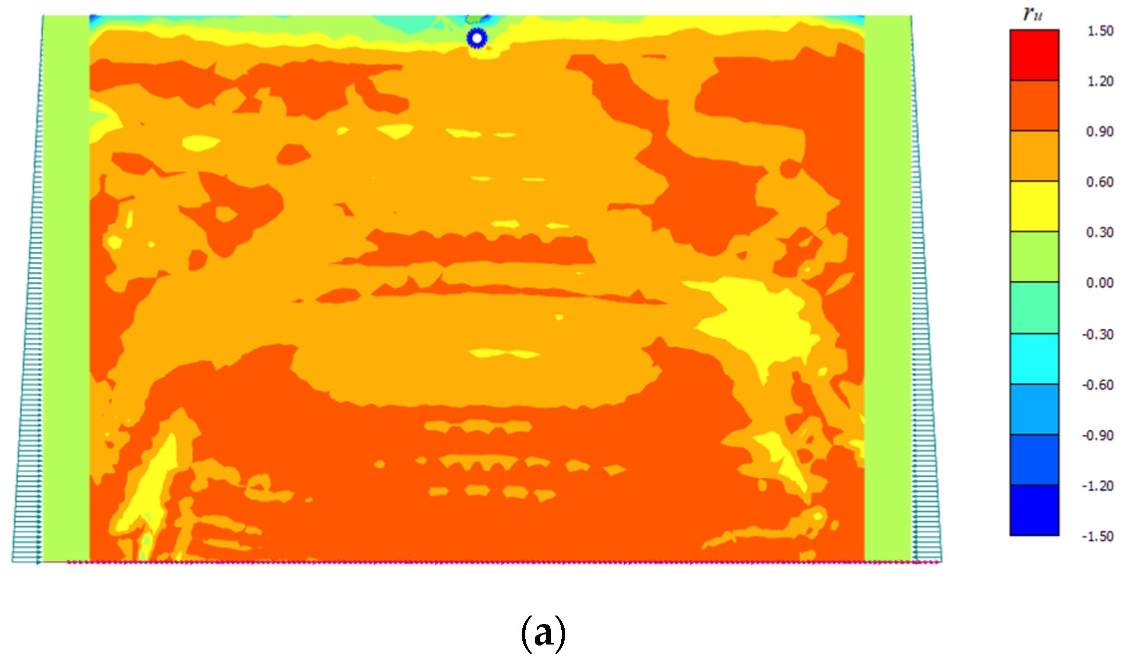
4.1. Liquefaction Potential of Soil Mass in the Earthquake Phase

In the earthquake phase, a dynamic loading (acceleration) is applied at the bottom of the soil mass to simulate the effect of a seismic event on a soil mass. The frequency of an earthquake can be between 0.01 to 10 Hz, and the amplitude can be well below 0.5 g (g is the gravitational acceleration) [46]. In this study, the frequency was considered to be 1 Hz, 2 Hz and 3Hz, and the amplitude was considered to be 0.05 g, 0.1 g, 0.3 g and 0.5 g. The variation of the liquefaction potential of the soil mass with the seismic frequency, seismic amplitude and soil relative density are shown in Figure 4, Figure 5 and Figure 6, respectively. In the PM4Sand model, the liquefaction potential is indicated by a user-defined parameter called the pore-pressure ratio (r_u), defined as:

$$r_u=1-\left({\sigma }_v/{\sigma }_{v0}\right)$$

(8)

where σ_v is the vertical stress and σ_v0 is the initial vertical stress at the beginning of a phase. The portion of the soil mass where r_u is 1 or higher is considered to be completely liquefied. The liquefaction potential of the soil is shown in Figure 4, Figure 5 and Figure 6 using pore water pressure maps.

The variation of the liquefaction potential with the frequency of the seismic input is shown in Figure 4. From these maps, it can be observed that zones with a color close to red have a high positive value of the pore water pressure ratio (r_u), which indicates a higher liquefaction potential. Figure 4a shows that, for a seismic frequency of 1 Hz, the majority of the soil mass is colored orange, which corresponds to pore water pressure ratios in the range of 0.9–1.2. On the other hand, when the seismic frequency is 3 Hz (Figure 4c), only a few soil areas have an orange color, and the majority of the soil mass has a light yellow color, which corresponds to a pore-water pressure ratio within the range of 0.3 to 0.6. A similar evolution of the pore pressure ratio was also observed for other soil densities and seismic amplitudes. Therefore, these results indicate that the pore water pressure ratio and, in turn, the liquefaction potential increase when the frequency of the seismic loading decreases.

The effect of the seismic amplitude on the liquefaction potential of the soil mass is shown in Figure 5. The results indicate that, for a 0.1 g amplitude (Figure 5a), the majority of the soil mass is colored orange, which means that most of the soil has liquefied (r_u = 0.9–1.2). By increasing the amplitude, the orange area reduces, and the area colored dark yellow (r_u = 0.6–0.9) is now dominant. In addition, the increment of the signal amplitude has a noticeable influence on the increment of the negative pore water pressure ratios (defined by the blue-colored areas of the soil). The occurrence of negative pore water pressure within the soil mass can be attributed to the dilation of the soil mass during vibration. A similar kind of dilation behavior of Nevada sand was also observed by Dinesh et al. [47]. Moreover, by comparing Figure 4 and Figure 5, it can also be observed that, for a given soil, the reduction in the liquefaction potential that is seen by increasing the amplitude is smaller than the one that is seen by increasing the frequency of the seismic signal. This result indicates that the liquefaction potential of a given soil mass is more sensitive to the frequency of the signal than to its amplitude.

Finally, the influence of seismic loading on the liquefaction potential of the soil is also explored for three different soil densities, as shown in Figure 6. It can be observed that, for the same earthquake signal (with a 0.1 g amplitude and a 1Hz frequency), the pore water pressure ratio is higher in the soil with a 40% relative density, in comparison to the case with a 60% relative density soil. From Figure 6a, it can be seen that for the 40% relative density soil, a large portion of the soil is liquefied (defined by the orange-colored area), while in Figure 6c, where a 60% relative density soil is used, only a few layers at the top are liquefied, and most of the soil mass has pore water pressure ratios within 0.6 to 0.9 (defined by the light yellow-colored areas). Thus, it can be concluded that, for a given seismic signal, the liquefaction potential decreases with the increase of the soil density.

4.2. Upheaval Displacement/Floatation of the Pipeline in the Earthquake Phase

During a seismic event, a pipeline is displaced from its original position. Depending on the apparent unit weight of the pipeline and the soil mass, the pipe can either settle (sink) or move upwards (float). In the current study, the floatation or upheaval displacement of the pipeline is explored. The variation of the pipe upheaval displacement with various combinations of soil and seismic parameters is discussed below.

The upheaval buckling of the pipeline during the earthquake stage was studied for a range of frequencies of dynamic loading, namely 1 Hz, 2 Hz, 3 Hz and 4Hz. The upheaval buckling of the pipeline that is obtained along the 30 s of the dynamic loading is plotted in Figure 7 for the considered frequencies of the seismic signal. Evidently, the upheaval displacement behavior of the pipeline depends on the earthquake event duration. During the initial 5 s of shaking, the upheaval buckling of the pipeline was higher for lower frequency loadings. A similar result was also observed by Azadi and Hosseini [38], who used an earthquake duration of 10 s. However, for a longer duration, the relationship between the upheaval displacement and the frequency of the earthquake changed. For the overall duration of 30 s, it was observed that the upheaval displacement of the pipeline reached the peak value more quickly for lower frequency loadings, while for higher frequency loadings, the peak of the pipe upheaval buckling took longer to be reached. From Figure 7, it can be observed that for a pipe embedment depth ratio of 3 and an acceleration amplitude of 0.1 g, the peak pipeline upheaval buckling corresponding to the 1 Hz frequency is 0.4 mm, and the peak is achieved at 3.44 s, while the peak pipeline upheaval buckling corresponding to a 2 Hz frequency is 18.3 mm, and it is achieved after 19.06 s. For the 3 Hz frequency, the peak upheaval buckling is not achieved even after 30 s of shaking. Moreover, the pipe is seen to start sinking after reaching the peak. A similar phenomenon was also observed for the other amplitudes and pipe embedment depths. In addition, the rate of sinking in the case of 1 Hz signal frequency was observed to be significantly higher.

The initial increase in the pipe upheaval buckling is due to the increase in the pore water pressure in the soil around the pipeline under dynamic loading. In addition, the soil around the pipeline is liquefied under the given dynamic loading, which causes an upward buoyancy force on the pipeline. The sinking of the pipeline that is seen after reaching a maximum value can be attributed to the settlement of the pipeline due to the readjustment of the soil particles. Moreover, from Figure 4 it can be observed that at a given duration (30 s), a soil body is more liquefied under a lower (1 Hz) seismic signal in comparison to the higher (2–3 Hz) seismic signals. Thus, it is understandable that for a lower frequency (1 Hz), the soil body reaches higher liquefaction potential at a faster rate. Moreover, the sinking of the pipeline can be explained from the readjustment properties of soil particles under vertical overburden stress. In case of a 1 Hz seismic frequency and a deeper embedment depth (10D), the combined pipe soil weight is very high, and the soil body becomes liquefied at a very short duration of the seismic event. Thus, under the combined effects of the signal frequency and the pipe-soil weight, a very rapid sinking of the pipeline is observed in case of the said situation.

Several authors observed an increase in the upheaval buckling of the pipeline with increasing seismic signal amplitudes [48]. However, several authors also observed a decrease in the pipeline upheaval buckling [49]. In the current study, the variation of the upheaval displacement of the pipeline with the amplitude of the seismic signal is given in Figure 8. The amplitude is given as a multiplier of g (gravitational acceleration), and the pipe upheaval buckling is given in mm. From Figure 8, it can be observed that the upheaval displacement of the pipeline decreased when the amplitude was increased up to 0.3 g. However, the upheaval displacement increased with further increments of the seismic amplitude from 0.3 g to 0.5 g. Such behavior of the upheaval displacement can be attributed to the variation of liquefaction potential around the pipe with the variation of the seismic signal amplitude. Moreover, it can be observed that the influence of the signal amplitude on the upheaval displacement of the pipeline is more prominent for the shallow embedment depth case, as compared to the deeper embedment depth case. The overburdened soil pressure is high for deeply embedded pipelines that restrict the pipeline’s upheaval movement. However, a shallow embedded pipeline is subjected to minimal soil overburden loading, and thus is greatly influenced by the signal parameters.

The variation of the upheaval displacement or uplift of a pipeline with the embedment depth is plotted in Figure 9. In this figure, it can be observed that the upheaval buckling of the pipeline decreased when the embedment depth is increased. Moreover, it is also noticeable that this drop in the upheaval buckling of the pipeline is sharper when the frequency of the earthquake signal is higher. For example, for a 40% relative density of the sand and a 0.1 g amplitude of the earthquake signal, the reduction of the upheaval buckling is 68.7% for a seismic frequency of 2 Hz when the embedment depth increases from 1 m to 5 m, while the reduction in the pipe upheaval buckling is 85.6% for a similar increase of the pipe embedment depth and a seismic signal with a 3 Hz frequency. A similar decrease is also observed for other seismic amplitudes and soil relative densities. Saeedzadeh and Hataf [29] also observed a decreasing trend of the pipe upheaval displacement when increasing the embedment depth.

Regarding the effect of the pipe embedment depth, since the volume of soil above the pipeline increases when the pipe embedment depth is increased, the weight of the soil block above the pipeline and the shear strength at the failure zone also increased. In turn, the resistance against the pipe upheaval displacement also increased. Hence, the upheaval displacement of the pipeline decreases when the pipe embedment depth was increased.

To study the effect of the soil density on the upheaval displacement of pipelines under earthquake loading, three different densities of the Nevada sand are considered, namely with density indices of 40%, 50% and 60%. In Figure 10, the upheaval displacement of the pipeline is plotted with the density of the sand for a seismic amplitude of 0.1 g and different pipe embedment depths and seismic frequencies. In this figure, it can be observed that the upheaval displacement of the pipeline increases when the soil density is increased, and also for the 1 Hz and 2 Hz seismic signals. However, for the 3 Hz frequency, the upheaval displacement of the pipeline increases with the relative density of the soil only up to a certain point, after which it decreases again.

In liquefied soil, a buoyancy force is applied to the pipeline. The buoyancy force acting on pipelines increases with the increase in the excess pore pressure, and facilitates the upheaval buckling of the pipeline [50]. From Figure 10, it can be observed that the pore pressure ratio is very high for the given seismic loading, and a large section of the soil mass is close to liquefaction. Again, for liquefied soil, the buoyancy force acting on the embedded pipeline is given as:

F_buoyancy = ρ_sat · g · v

(9)

where ρ_sat is the saturated density of soil, g is the gravitational acceleration, and v is the pipe volume [40]. Therefore, the buoyancy force increases when the soil density is increased, which causes an increase in the upheaval buckling of the pipeline. Moreover, it can also be observed from Figure 4 that the pore pressure ratio (r_u) decreased considerably when the frequency of the seismic loading is increased. Hence, the buoyancy force acting on the pipeline also decreased. Again, when increasing the unit weight of the soil, the weight of the soil block above the pipeline also increases and possibly exceeds the buoyancy force acting on the pipeline, thus causing a decrease in the upheaval buckling of the pipeline for the 3 Hz signal and the 60% soil relative density.

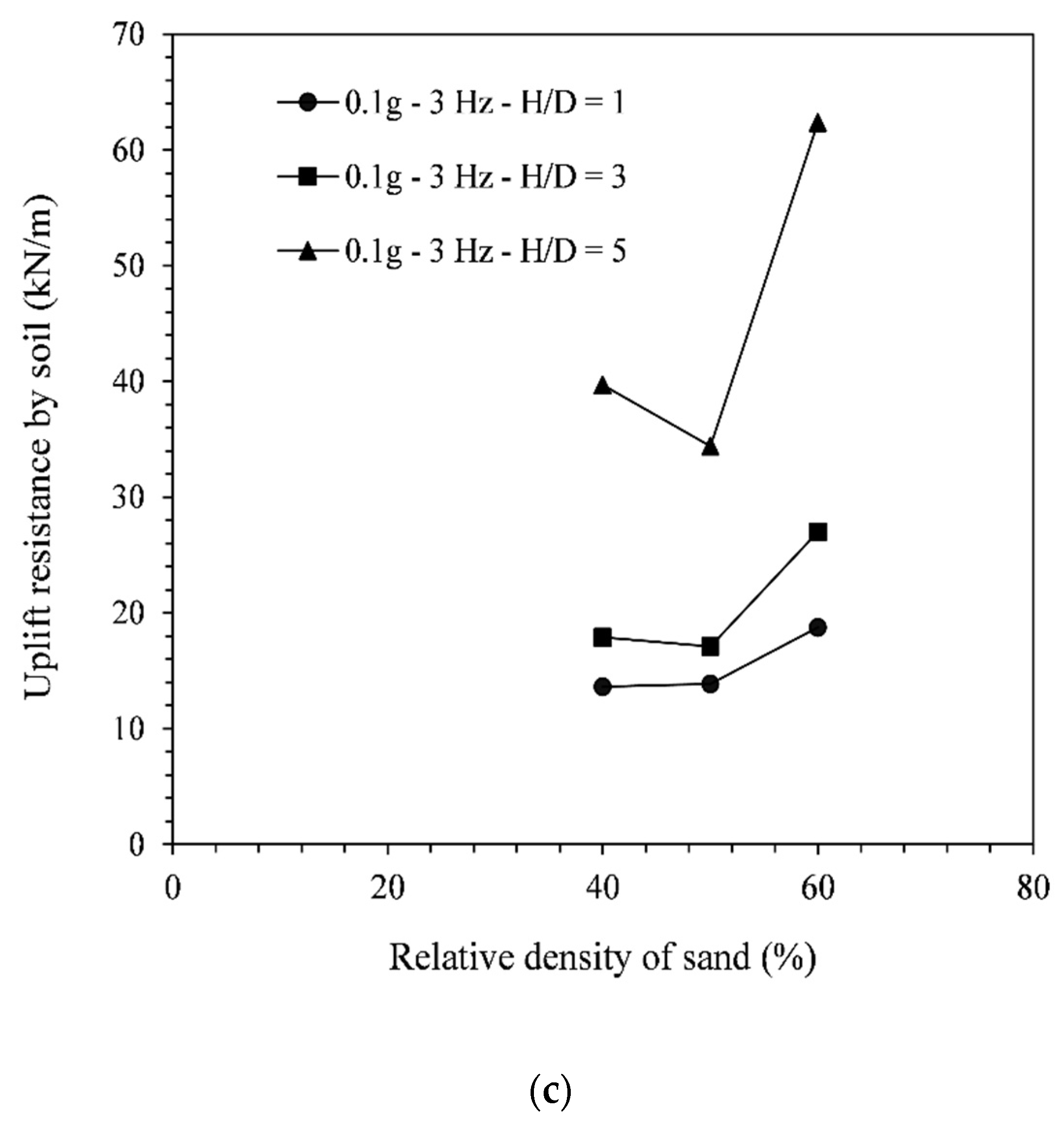
4.3. Post-Earthquake Uplift Resistance

In this phase, the pipe is considered to buckle in an upward direction under drained conditions. Thus, an upward nodal displacement is applied to the pipeline to obtain the resistance force on the pipeline. This section aims to explore the resistance of the soil against the pipe upheaval displacement at the post-earthquake stage. The amplitude and frequency of the seismic signal, the soil density and the pipe embedment depth are varied to obtain the variation of the uplift resistance of the soil on the pipeline.

The variation of the uplift capacity factor with the seismic loading frequency is shown in Figure 11. The vertical axes of the graphs represent the uplift resistance on the pipeline, while the horizontal axes represent the frequency of the seismic signal. In Figure 11, the uplift resistance of an offshore pipeline show an overall increasing trend with increasing seismic signal frequency. The increase in the uplift resistance of the soil can be attributed to the densification of the soil at the post-shake stage as a result of the seismic loading at the prior stage. Moreover, it can also be observed that the pipelines with deeper embedment depth showed a sharper increase in uplift resistance with increasing signal frequency, compared to the pipelines with shallow embedment depth. For example, in Figure 11a, for an embedment ratio of 10, the increment in uplift resistance is 619.4% for an increase in seismic signal frequency from 1 to 4 Hz. However, the increment in uplift resistance for an embedment depth ratio of 1 is only 92.8% for the same increase in signal frequency. The reason for such a phenomenon can be described using Figure 4. The zone with higher liquefaction potential shifts towards the upper layer with increasing signal frequency. Thus, for a higher frequency (3–4 Hz), the upper layers of the soil-body remained liquefied, while the liquefaction potential decreased drastically at the deeper layer. Smaller liquefaction potential indicates a lesser loss of soil shear strength. Thus, the uplift resistance at the deeper soil layer increased sharply with increasing seismic signal frequency. The uplift resistance at the shallow soil layer showed a comparatively slower increment rate.

The dependency of the post-shake uplift resistance on the seismic signal amplitude is shown in Figure 12 for different seismic frequencies and pipe embedment depths. It can be observed that the relationship between the uplift resistance and the seismic amplitude depends on the signal frequency and on the pipe embedment depth. In the same figure, it can also be observed that initially, the uplift resistance decreased with increasing seismic signal amplitude, until it reached the lowest value. Thereafter, the uplift resistance started increasing. For example, in Figure 12a, the uplift resistance corresponding to the 3 Hz frequency already reached the lowest value at a seismic amplitude of 0.1 g; while, the uplift resistance for other signal frequencies did not reach the lowest point within the considered range of the signal amplitude. Similarly, in Figure 12c, the plots of uplift resistance for the 2 Hz and 3 Hz signal frequencies reached the minima followed by an increase in uplift resistance. However, the uplift resistance corresponding to the 1 Hz signal frequency is yet to reach the lowest magnitude.

The variation of the post-peak uplift resistance of the Nevada sand with the pipeline embedment depth is shown in Figure 13. The abscissa represents the pipeline embedment depth, while the ordinate represents the post-shake uplift resistance of the pipeline.

It can be observed that, irrespective of the soil and seismic signal parameters, the post-peak uplift resistance increased with an increase in the embedment depth. With the increase in embedment depth, the boundary of the failure surface and the soil volume above the pipeline increased. Thus, the shear resistance along the failure boundary and the weight of the failed soil wedge also increased, which resulted in an increase in the uplift resistance of the soil.

The effect of the relative density of the Nevada sand on the post-shake uplift resistance of the sand is shown in Figure 14. It can be observed from Figure 14a that the uplift resistance of the soil increases when increasing the relative density of the soil for the 0.1 g and 1 Hz seismic signal. However, for an amplitude of 0.1 g and frequencies of 2 Hz and 3 Hz, the uplift resistance of the soil initially decreased for an increase in the soil relative density of 40% to 50%, while it then increases for a subsequent increase of 50% to 60%. The possible reason of this phenomenon is discussed in the following section.

In the post-shake stage, the soil is generally liquefied and has lost the shear strength. Thus, there are two major factors which determines the uplift resistance of the soil. The combined weight of the pipe and the soil above it contribute to the uplift resistance, while an upward buoyant force induced by the liquefied soil works against the uplift resistance. Both the weight of the soil above the pipeline and the buoyant force increases when the soil density is increased. However, the buoyant force also depends on the degree of soil liquefaction. The buoyant force induced by a partially liquefied soil is lower than the buoyant force induced by a completely liquefied soil [33]. From Figure 6 it can be observed that the liquefaction potential at the upper layers increases when the soil density is increased. Due to this enhanced liquefaction potential at the upper layer, the buoyant force increased and became predominant when the soil density was increased from 40% to 50%. However, when the soil density was increased from 50% to 60%, the overall liquefaction potential of the soil mass decreased and the weight of the soil above the pipeline became predominant. Thus, the uplift resistance of the soil further increased when the soil relative density was increased from 50% to 60%.

5. Conclusions

A numerical study was performed using the PLAXIS 2D software to analyze the behavior of an offshore pipeline as a function of several parameters. Specifically, the study examined the effect of several soil, pipeline and dynamic loading parameters on the liquefaction and post-shake uplift resistance of the soil around the pipeline and on the upheaval buckling of the pipeline. The parameters that were varied to perform the parametric study are the soil relative density, the pipe embedment depth, and the frequency and amplitude of the seismic signal. Two major phases were involved in the analyses (the earthquake and the post-earthquake phases) to examine in more detail the upheaval buckling of the pipeline within a liquefied soil, and the post-shaking uplift resistance of the soil. Moreover, to better understand the buckling behavior of a pipeline within a liquefied soil, the liquefaction potential of the soil mass under different signals and soil parameters was also analyzed. The following conclusions were extracted from the results of the study:

• The liquefaction potential of the soil mass depends on the amplitude and frequency of the seismic signal, and on the relative density of the soil. For a given soil, the liquefaction potential was seen to decrease with the increase in the frequency and the amplitude of the seismic signal. However, when the soil relative density increases, the liquefaction potential at the upper layer of the soil was seen to increase, while the liquefaction potential at the middle and bottom layers of the soil was seen to decrease;
• The peak upheaval buckling of the pipeline is higher when the frequency of the seismic signal is also higher. However, the time to reach the peak upheaval buckling also increased with the increase of the signal frequency. On the other hand, the pipeline upheaval buckling decreased or remained the same initially when the amplitude of the seismic signal was increased for the analyzed cases;
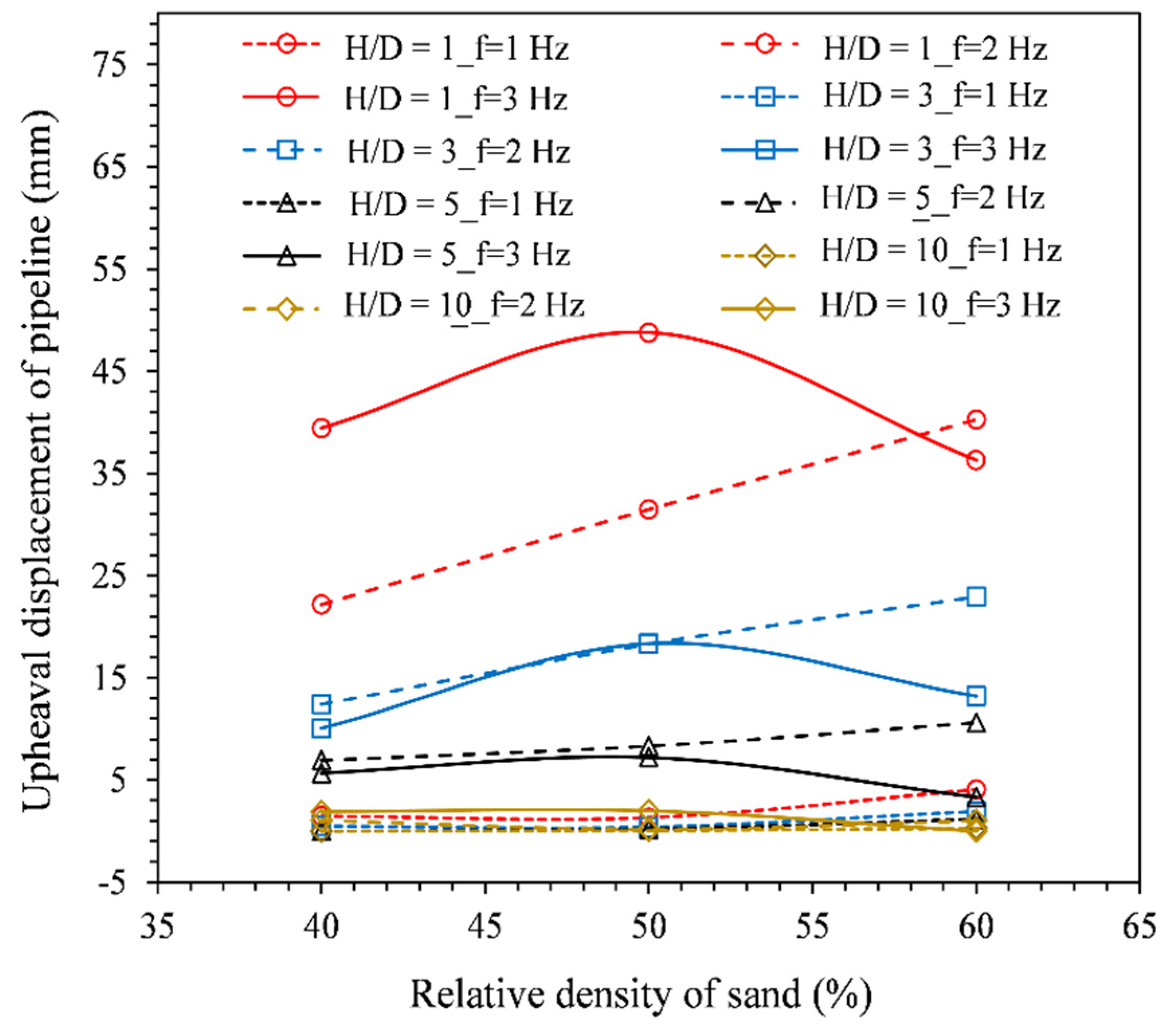
• The peak upheaval buckling of the pipeline was seen to consistently decrease when the embedment depth of the pipeline was increased. On the other hand, the relation between the pipeline upheaval buckling and the soil density was seen to also depend on the frequency of the seismic signal. For lower frequencies (1 Hz and 2 Hz), the upheaval buckling of the pipeline was seen to increase when the soil relative density was increased, while for a higher frequency (3 Hz) the pipeline upheaval buckling was higher for the mid value of the considered relative densities of the soil;
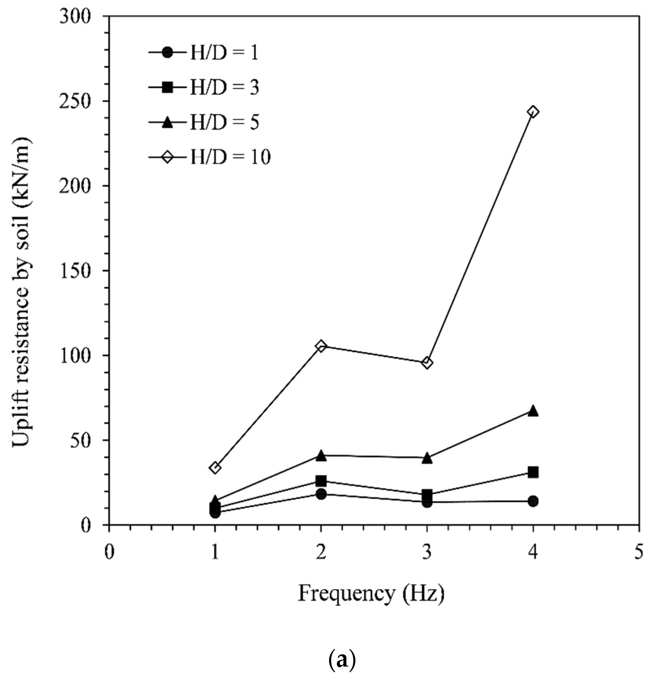
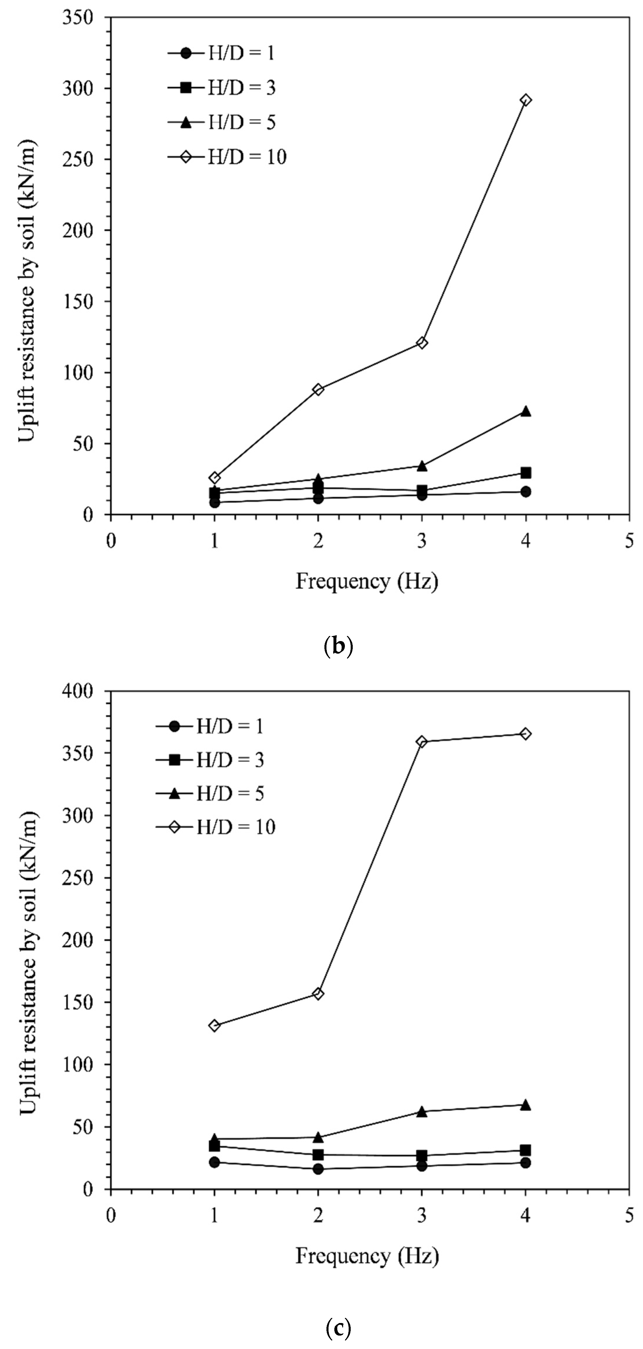
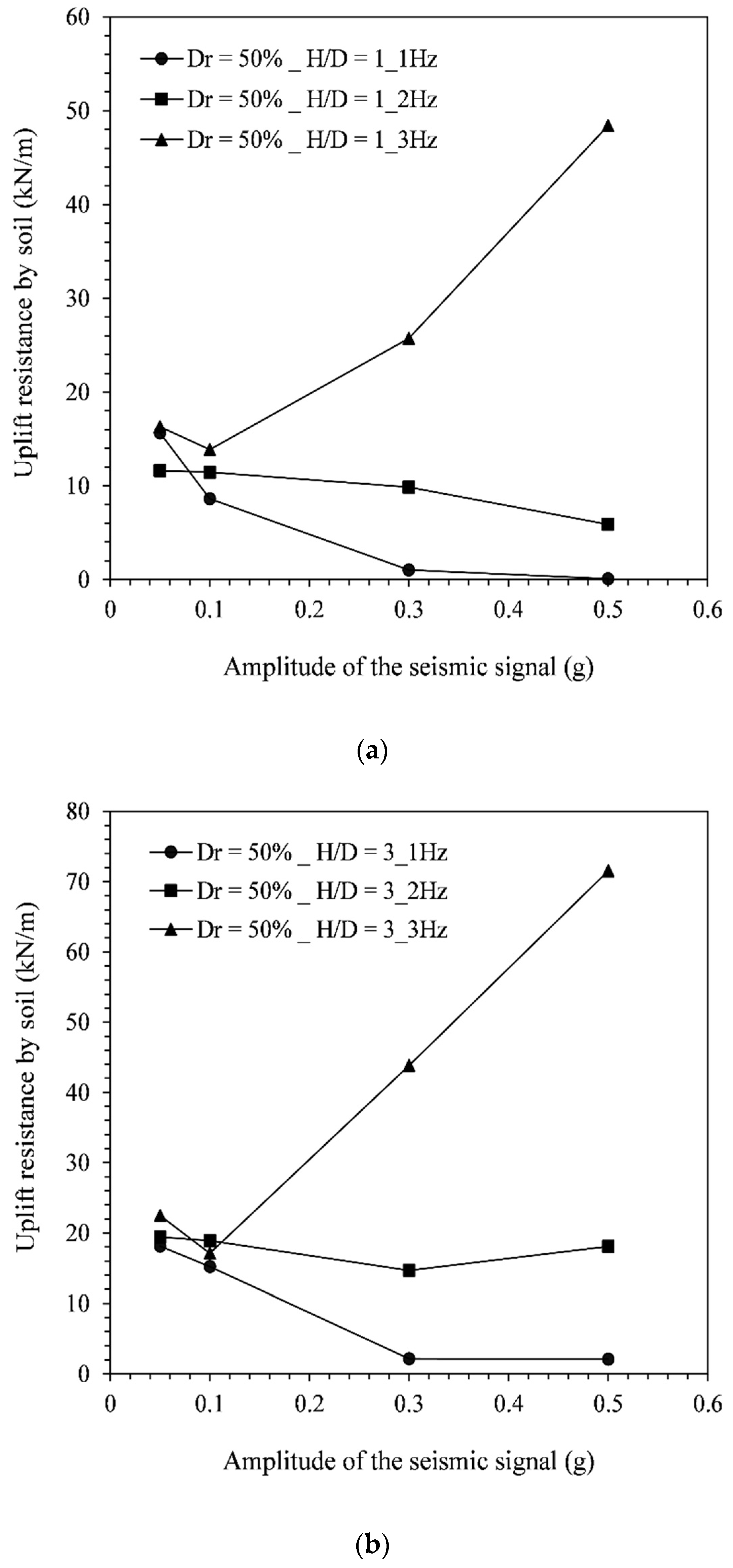
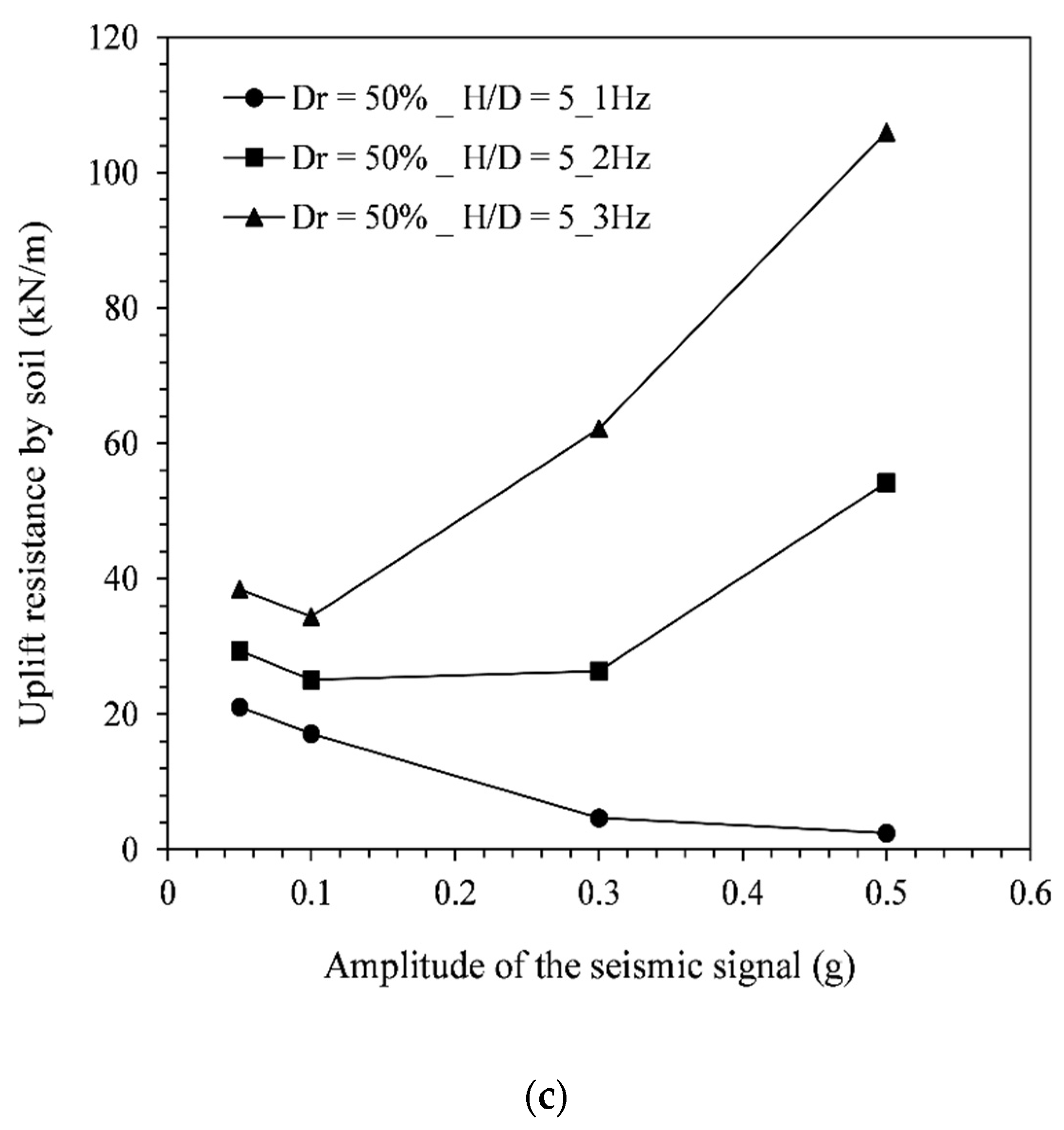
• The post-shake uplift resistance of the pipeline (V_up) showed an overall increasing trend with the seismic signal frequency. Moreover, the V_up initially decreased with the increasing seismic signal amplitude up to the lowest magnitude. After that, the V_up showed an increasing trend with the seismic signal amplitude. The relationship between V_up and signal amplitude is also observed to be influenced by the signal frequency and pipe embedment depth;
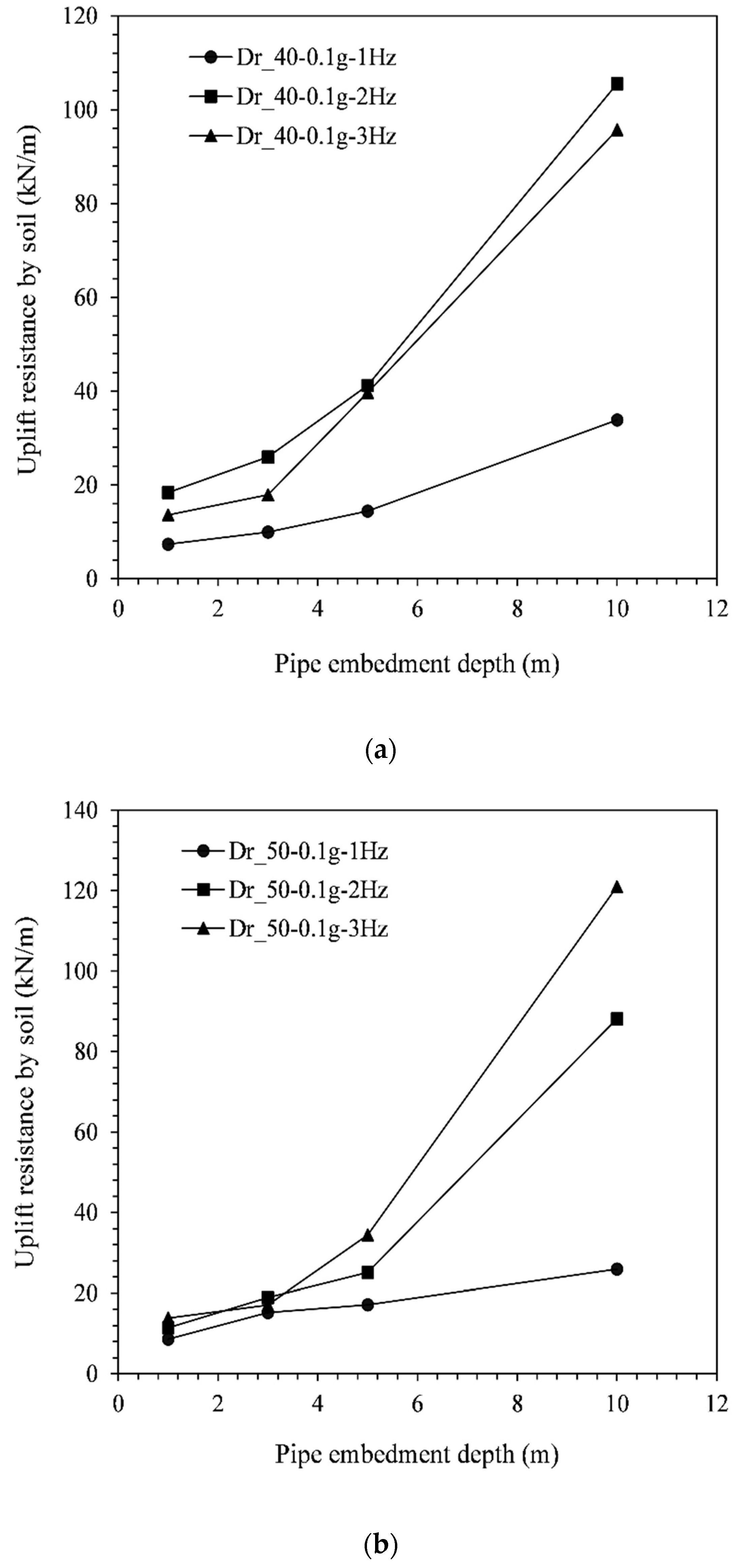
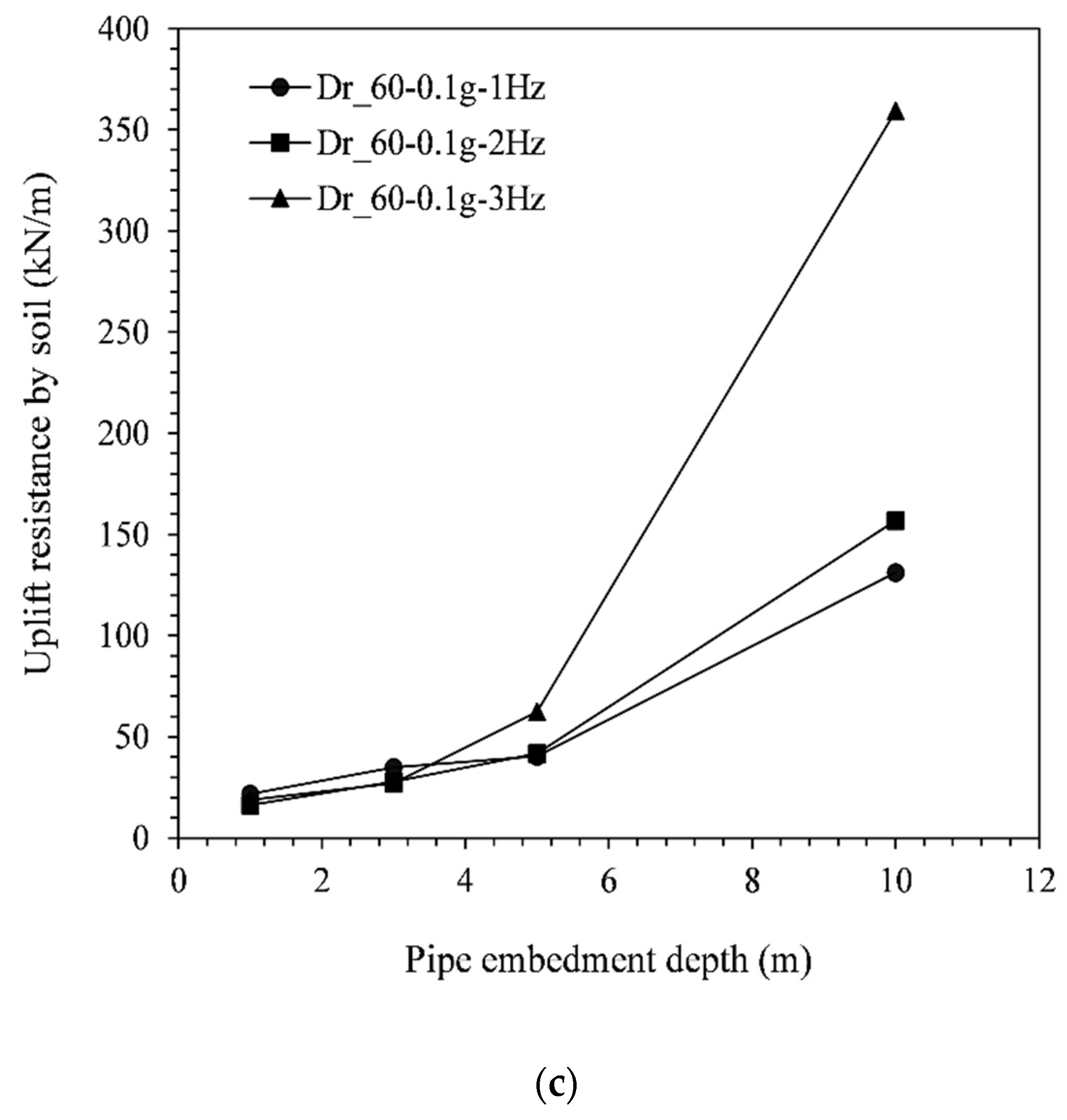
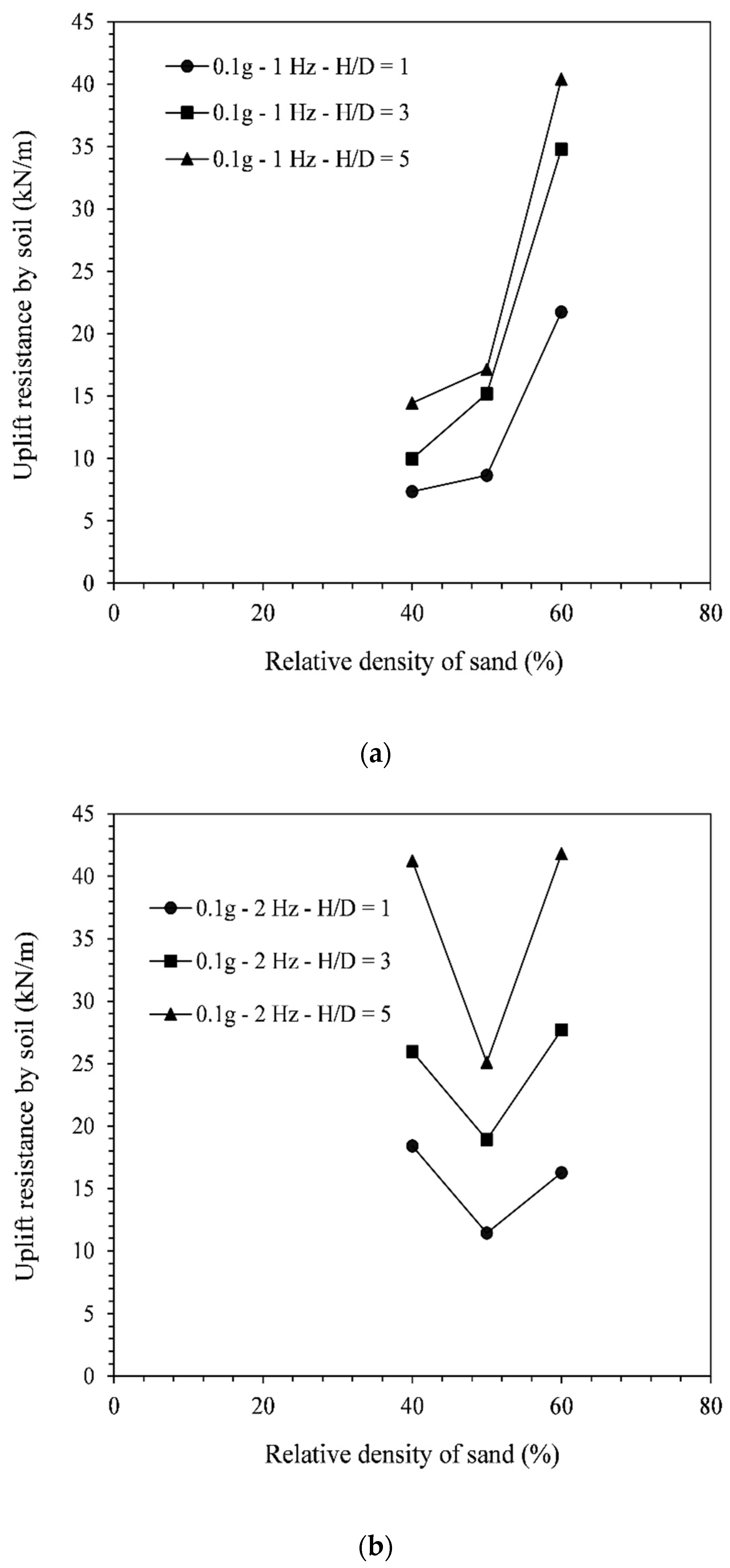
• The post-shake uplift resistance of the pipeline was seen to increase when increasing the embedment depth, and this variation was found to be independent of the seismic signal. However, the variation of V_up with the soil relative density was found to depend on the frequency of the seismic signal. For the lowest frequency (1 Hz), V_up increased when the soil density was increased, while for higher frequencies, V_up may decrease or increase when the soil density was increased.

Based on these conclusions, some of the parameters were seen to have non-uniform impacts on the soil and pipeline behavior. As such, it is suggested that additional studies similar to the one presented herein should be carried out using both small strain [40] and large displacement/deformation techniques [51,52,53]. The additional studies should further explore the relation between some of the selected parameters on the response of offshore pipelines in liquefiable soils, and should include the influence of other factors (e.g., the diameter of the pipeline or the duration of the earthquake signal). Furthermore, the behavior of offshore pipelines under earthquake signals simulated by real earthquake ground motions recorded in offshore conditions should also be analyzed. Such studies would provide a better understanding of the influence of earthquake loading characteristics that cannot be captured using sinusoidal wave loadings as considered herein [54,55]. It is also highlighted that the present research can also benefit from the application of pipelines and submarine cables. These are used for numerous other applications in ocean engineering for the oil and gas industry, and also the rising sector of marine renewable energy, such as the ones compiled in Fazeres-Ferradosa et al. [56,57] or in Taveira-Pinto et al. [58].

References

1. Maitra, S.; Chatterjee, S.; Choudhury, D. Generalized framework to predict undrained uplift capacity of buried offshore pipelines. Can. Geotech. J. 2016, 53, 1841–1852. [Google Scholar] [CrossRef]
2. Seth, D.; Manna, B.; Kumar, P.; Shahu, J.T.; Fazeres-Ferradosa, T.; Taveira-Pinto, F.; Rosa-Santos, P.; Carvalho, H. Uplift and lateral buckling failure mechanisms of offshore pipes buried in normally consolidated clay. Eng. Fail. Anal. 2021, 121, 105161. [Google Scholar] [CrossRef]
3. Seth, D.; Manna, B.; Shahu, J.T.; Fazeres-Ferradosa, T.; Pinto, F.T.; Rosa-Santos, P.J. Buckling Mechanism of Offshore Pipelines: A State of the Art. J. Mar. Sci. Eng. 2021, 9, 1074. [Google Scholar] [CrossRef]
4. Schiff, A.J. Northridge Earthquake: Lifeline Performance and Post-Earthquake Response; ASCE: New York, NY, USA, 1995. [Google Scholar]
5. Chou, H.S.; Yang, C.Y.; Hsieh, B.J.; Chang, S.S. A study of liquefaction related damages on shield tunnels. Tunn. Undergr. Space Technol. 2001, 16, 185–193. [Google Scholar] [CrossRef]
6. Murray, E.J.; Geddes, J.D. Uplift of anchor plates in sand. J. Geotech. Eng. 1987, 113, 202–215. [Google Scholar] [CrossRef]
7. Singh, S.P.; Tripathy, D.P.; Ramaswamy, S.V. Estimation of uplift capacity of rapidly loaded plate anchors in soft clay. Mar. Georesour. Geotechnol. 2007, 25, 237–249. [Google Scholar] [CrossRef]
8. Newson, T.A.; Deljoui, P. Finite element modelling of upheaval buckling of buried offshore pipelines in clayey soils. Soil Rock Behav. Model. 2006, 351–358. [Google Scholar]
9. Liu, R.; Xiong, H.; Wu, X.; Yan, S. Numerical studies on global buckling of subsea pipelines. Ocean. Eng. 2014, 78, 62–72. [Google Scholar] [CrossRef]
10. Schotman, G.J.M.; Stork, F.G. Pipe-soil interaction: A model for laterally loaded pipelines in clay. In Offshore Technology Conference; OnePetro: Richardson, TX, USA, 1987. [Google Scholar]
11. El-Gharbawy, S. Uplift capacity of buried offshore pipelines. In Proceedings of the Sixteenth International Offshore and Polar Engineering Conference, San Francisco, CA, USA, 28 May–2 June 2006; OnePetro: Richardson, TX, USA, 2006. [Google Scholar]
12. Gao, X.F.; Liu, R.; Yan, S.W. Model test based soil spring model and application in pipeline thermal buckling analysis. China Ocean. Eng. 2011, 25, 507–518. [Google Scholar] [CrossRef]
13. Liu, R.; Yan, S.; Wu, X. Model test studies on soil restraint to pipeline buried in Bohai soft clay. J. Pipeline Syst. Eng. Pract. 2013, 4, 49–56. [Google Scholar] [CrossRef]
14. Randolph, M.F.; Houlsby, G.T. The limiting pressure on a circular pile loaded laterally in cohesive soil. Geotechnique 1984, 34, 613–623. [Google Scholar] [CrossRef]
15. Schaminee, P.E.L.; Zorn, N.F.; Schotman, G.J.M. Soil response for pipeline upheaval buckling analyses: Full-scale laboratory tests and modelling. In Offshore Technology Conference; OnePetro: Richardson, TX, USA, 1990. [Google Scholar]
16. Liu, R.; Basu, P.; Xiong, H. Laboratory tests and thermal buckling analysis for pipes buried in Bohai soft clay. Mar. Struct. 2015, 43, 44–60. [Google Scholar] [CrossRef]
17. Chen, R.P.; Zhu, B.; Ni, W.J. Uplift tests on full-scale pipe segment in lumpy soft clay backfill. Can. Geotech. J. 2016, 53, 578–588. [Google Scholar] [CrossRef]
18. Seth, D.; Manna, B.; Shahu, J.T.; Fazeres-Ferradosa, T.; Taveira-Pinto, F.; Rosa-Santos, P.; Pinto, F.V.T. Offshore pipeline buried in Indian coastal clay: Buckling behaviour analysis. Ships Offshore Struct. 2021, 1–16. [Google Scholar] [CrossRef]
19. Merifield, R.; White, D.J.; Randolph, M.F. The ultimate undrained resistance of partially embedded pipelines. Géotechnique 2008, 58, 461–470. [Google Scholar] [CrossRef]
20. Trautmann, C.H. Behavior of Pipe in Dry Sand under Lateral and Uplift Loading. Ph.D. Thesis, Cornell University, New York, NY, USA, 1983. [Google Scholar]
21. Robert, D.J.; Thusyanthan, N.I. Numerical and experimental study of uplift mobilization of buried pipelines in sands. J. Pipeline Syst. Eng. Pract. 2015, 6, 04014009. [Google Scholar] [CrossRef] [Green Version]
22. Roy, K.; Hawlader, B.; Kenny, S.; Moore, I. Uplift failure mechanisms of pipes buried in dense sand. Int. J. Geomech. 2018, 18, 04018087. [Google Scholar] [CrossRef]
23. Cheuk, C.Y.; White, D.J.; Bolton, M.D. Deformation mechanisms during uplift of buried pipes in sand. In Proceedings of the 16th International Conference on Soil Mechanics and Geotechnical Engineering, Osaka, Japan, 19–21 April 2005; IOS Press: Amsterdam, The Netherlands, 2005; pp. 1685–1688. [Google Scholar]
24. Cheuk, C.Y.; Take, W.A.; Bolton, M.D.; Oliveira, J.R.M.S. Soil restraint on buckling oil and gas pipelines buried in lumpy clay fill. Eng. Struct. 2007, 29, 973–982. [Google Scholar] [CrossRef]
25. Kumar, P.; Seth, D.; Manna, B.; Shahu, J.T. Lateral and Uplift Capacity of Pipeline Buried in Seabed of Homogeneous Clay. J. Pipeline Syst. Eng. Pract. 2021, 12, 04021020. [Google Scholar] [CrossRef]
26. Pedersen, P.T.; Jensen, J.J. Upheaval creep of buried heated pipelines with initial imperfections. Mar. Struct. 1988, 1, 11–22. [Google Scholar] [CrossRef]
27. Wang, Y.; Zhang, X.; Zhao, Y.; Chen, H.; Duan, M.; Estefen, S.F. Perturbation analysis for upheaval buckling of imperfect buried pipelines based on nonlinear pipe-soil interaction. Ocean. Eng. 2017, 132, 92–100. [Google Scholar] [CrossRef]
28. Ling, H.I.; Sun, L.; Liu, H.; Mohri, Y.; Kawabata, T. Finite element analysis of pipe buried in saturated soil deposit subject to earthquake loading. J. Earthq. Tsunami 2008, 2, 1–17. [Google Scholar] [CrossRef]
29. Saeedzadeh, R.; Hataf, N. Uplift response of buried pipelines in saturated sand deposit under earthquake loading. Soil Dyn. Earthq. Eng. 2011, 31, 1378–1384. [Google Scholar] [CrossRef]
30. Wang, L.R.L.; Shim, J.S.; Ishibashi, I.; Wang, Y. Dynamic responses of buried pipelines during a liquefaction process. Soil Dyn. Earthq. Eng. 1990, 9, 44–50. [Google Scholar] [CrossRef]
31. Maotian, L.; Xiaoling, Z.; Qing, Y.; Ying, G. Numerical analysis of liquefaction of porous seabed around pipeline fixed in space under seismic loading. Soil Dyn. Earthq. Eng. 2009, 29, 855–864. [Google Scholar] [CrossRef]
32. Azadi, M.; Hosseini, S.M.M. Analyses of the effect of seismic behavior of shallow tunnels in liquefiable grounds. Tunn. Undergr. Space Technol. 2010, 25, 543–552. [Google Scholar] [CrossRef]
33. Huang, B.; Liu, J.; Lin, P.; Ling, D. Uplifting behavior of shallow buried pipe in liquefiable soil by dynamic centrifuge test. Sci. World J. 2014, 2014, 838546. [Google Scholar] [CrossRef]
34. Sharafi, H.; Parsafar, P. Seismic simulation of liquefaction-induced uplift behavior of buried pipelines in shallow ground. Arab. J. Geosci. 2016, 9, 215. [Google Scholar] [CrossRef]
35. Kutanaei, S.S.; Choobbasti, A.J. Prediction of liquefaction potential of sandy soil around a submarine pipeline under earthquake loading. J. Pipeline Syst. Eng. Pract. 2019, 10, 04019002. [Google Scholar] [CrossRef]
36. Ling, H.I.; Mohri, Y.; Kawabata, T.; Liu, H.; Burke, C.; Sun, L. Centrifugal modeling of seismic behavior of large-diameter pipe in liquefiable soil. J. Geotech. Geoenviron. Eng. 2003, 129, 1092–1101. [Google Scholar] [CrossRef]
37. Kutanaei, S.S.; Choobbasti, A.J. Effect of the fluid weight on the liquefaction potential around a marine pipeline using CVFEM. EJGE 2013, 18, 633–646. [Google Scholar]
38. Chian, S.C.; Madabhushi, S.P.G. Effect of buried depth and diameter on uplift of underground structures in liquefied soils. Soil Dyn. Earthq. Eng. 2012, 41, 181–190. [Google Scholar] [CrossRef]
39. Boulanger, R.W.; Ziotopoulou, K. PM4Sand (Version 3.1): A Sand Plasticity Model for Earthquake Engineering Applications; Report No. UCD/CGM-17/01; Center for Geotechnical Modeling, Department of Civil and Environmental Engineering, University of California, Davis: Davis, CA, USA, 2017. [Google Scholar]
40. Brinkgreve, R.B.J.; Kumarswamy, S.; Swolfs, W.M.; Waterman, D.; Chesaru, A.; Bonnier, P.G. PLAXIS 2016; PLAXIS B.V.: Delft, The Netherlands, 2016. [Google Scholar]
41. Vilhar, G.; Brinkgreve, R. Plaxis the PM4Sand Model; PLAXIS B.V.: Delft, The Netherlands, 2018. [Google Scholar]
42. Minga, E.; Burd, H.J. Validation of the PLAXIS MoDeTo 1D Model for Dense Sand. 2019. Available online: https://communities.bentley.com/products/geotech-analysis/w/plaxis-soilvision-wiki/45423/validation-report-of-plaxis-modeto-based-on-the-dunkirk-sand-pisa-field-tests (accessed on 25 June 2022).
43. Bray, J.D.; Luque, R. Seismic performance of a building affected by moderate liquefaction during the Christchurch earthquake. Soil Dyn. Earthq. Eng. 2017, 102, 99–111. [Google Scholar] [CrossRef]
44. Ziotopoulou, K. Seismic response of liquefiable sloping ground: Class A and C numerical predictions of centrifuge model responses. Soil Dyn. Earthq. Eng. 2018, 113, 744–757. [Google Scholar] [CrossRef]
45. Millen, M.D.L.; Rios, S.; Quintero, J.; da Fonseca, A.V. Prediction of time of liquefaction using kinetic and strain energy. Soil Dyn. Earthq. Eng. 2020, 128, 105898. [Google Scholar] [CrossRef]
46. Tosi, P.; Sbarra, P.; De Rubeis, V. Earthquake sound perception. Geophys. Res. Lett. 2012, 39, 24. [Google Scholar] [CrossRef]
47. Dinesh, N.; Banerjee, S.; Rajagopal, K. Performance evaluation of PM4Sand model for simulation of the liquefaction remedial measures for embankment. Soil Dyn. Earthq. Eng. 2022, 152, 107042. [Google Scholar] [CrossRef]
48. Sasaki, T.; Tamura, K. Prediction of liquefaction-induced uplift displacement of underground structures. In Proceedings of the 36th Joint Meeting US-Japan Panel on Wind and Seismic Effects, Gaithersburg, MD, USA, 17–22 May 2004. [Google Scholar]
49. Castiglia, M. The Experimental Study of Buried Onshore Pipelines Seismic-Liquefaction Induced Vertical Displacement in Shaking Table Tests and Its Remedial Measures. Ph.D. Thesis, University of Molise, Campobasso, Italy, 2019. [Google Scholar]
50. Kitaura, M.; Miyajima, M.; Suzuki, H. Response analysis of buried pipelines considering rise of ground water table in liquefaction processes. Doboku Gakkai Ronbunshu 1987, 1987, 173–180. [Google Scholar] [CrossRef] [Green Version]
51. Kong, D. Quantifying Residual Resistance of Light Pipelines during Large-Amplitude Lateral Displacement Using Sequential Limit Analysis. J. Geotech. Geoenviron. Eng. 2022, 148, 04022054. [Google Scholar] [CrossRef]
52. Sabetamal, H. Finite Element Algorithms for Dynamic Analysis of Geotechnical Problems. Ph.D. Thesis, The University of Newcastle, Newcastle, Australia, 2015. [Google Scholar]
53. Dutta, S.; Hawlader, B.; Phillips, R. Finite element modeling of partially embedded pipelines in clay seabed using Coupled Eulerian–Lagrangian method. Can. Geotech. J. 2015, 52, 58–72. [Google Scholar] [CrossRef]
54. Chen, B.; Wang, D.; Li, H.; Sun, Z.; Shi, Y. Characteristics of earthquake ground motion on the seafloor. J. Earthq. Eng. 2015, 19, 874–904. [Google Scholar] [CrossRef]
55. Chen, B.; Wang, D.; Chen, S.; Hu, S. Influence of site factors on offshore ground motions: Observed Results and Numerical Simulation. Soil Dyn. Earthq. Eng. 2021, 145, 106729. [Google Scholar] [CrossRef]
56. Fazeres-Ferradosa, T.; Rosa-Santos, P.; Taveira-Pinto, F.; Vanem, E.; Carvalho, H.; Correia, J. Editorial: Advanced research on offshore structures and foundation design: Part 1: Proceedings of the Institution of Civil Engineers. In Maritime Engineering; Thomas Telford Ltd.: London, UK, 2019; Volume 172, pp. 118–123. [Google Scholar] [CrossRef]
57. Fazeres-Ferradosa, T.; Rosa-Santos, P.; Taveira-Pinto, F.; Pavlou, D.; Gao, F.-P.; Carvalho, H.; Oliveira-Pinto, S. Preface: Advanced Research on Offshore Structures and Foundation Design: Part 2 Proceedings of the Institution of Civil Engineers. In Maritime Engineering; Thomas Telford Ltd.: London, UK, 2020; Volume 173, pp. 96–99. [Google Scholar] [CrossRef]
58. Taveira-Pinto, F.; Rosa-Santos, P.; Fazeres-Ferradosa, T. Marine renewable energy. Renew. Energy 2020, 150, 1160–1164. [Google Scholar] [CrossRef]
Figure 1. Schematic diagram of the 2D section of the pipeline buried in a granular seabed, and the forces and displacements applied to it.
Energies 15 05561 g001
Figure 2. A typical discretized soil volume with two drained zones on the two sides.
Energies 15 05561 g002
Figure 3. Comparison of the pipe upheaval buckling obtained from the current study and past studies under dynamic loading [28,29,36].
Energies 15 05561 g003
Figure 4. Liquefaction potential of soil with 50% relative density and a seismic signal of 0.1 g amplitude and (a) 1 Hz, (b) 2 Hz, and (c) 3 Hz frequency.
Energies 15 05561 g004
Figure 5. Liquefaction potential of soil with 50% relative density and a seismic signal of 1 Hz frequency and (a) 0.1 g, (b) 0.3 g, and (c) 0.5 g amplitudes.
Energies 15 05561 g005
Figure 6. Liquefaction potential of soil under a seismic signal of 1 Hz frequency and 0.1 g amplitude and with a relative density of (a) 40%, (b) 50% and (c) 60%.
Energies 15 05561 g006aEnergies 15 05561 g006b
Figure 7. Upheaval displacement of the pipeline buried within a Nevada sand of 50% relative density and under a seismic event with a 0.1 g amplitude.
Energies 15 05561 g007
Figure 8. Variation of the pipe upheaval displacement with the amplitude of the seismic signal for frequencies of (a) 1 Hz, (b) 2 Hz, and (c) 3 Hz.
Energies 15 05561 g008aEnergies 15 05561 g008b
Figure 9. Variation of the upheaval displacement of the pipeline with the embedment depth of the pipeline.
Energies 15 05561 g009
Figure 10. Variation of the upheaval displacement of the pipeline with the relative density of the sand.
Energies 15 05561 g010
Figure 11. Variation of the post-shake uplift resistance with the frequency of the seismic signal with a 0.1 g amplitude and a backfill soil with relative densities of (a) 40%, (b) 50% and (c) 60%.
Energies 15 05561 g011aEnergies 15 05561 g011b
Figure 12. Variation of the post-shake uplift resistance with the earthquake amplitude for different signal frequencies and pipeline embedment depth ratios (H/D) of (a) 1, (b) 3, and (c) 5.
Energies 15 05561 g012aEnergies 15 05561 g012b
Figure 13. Variation of the post-shake uplift resistance with the pipe embedment depth for different seismic signals and backfill soil densities of (a) 40%, (b) 50% and (c) 60%.
Energies 15 05561 g013aEnergies 15 05561 g013b
Figure 14. Variation of the post-shake uplift resistance with the relative density of the backfill soil for different pipe embedment depths, a seismic signal of amplitude 0.1 g and frequencies (a) 1 Hz, (b) 2 Hz and (c) 3 Hz.
Energies 15 05561 g014aEnergies 15 05561 g014b