A Novel Voltage Sag Detection Method Based on a Selective Harmonic Extraction Algorithm for Nonideal Grid Conditions

Abstract

Voltage sag detection is utilized to capture the sag occurrence moment and calculate the sag depth of power grid voltage in real time, so as to generate reference voltage for controlling voltage interactive equipment such as dynamic voltage restorers (DVRs). However, the traditional voltage sag detection methods based on synchronously rotating frames (SRFs) are unable to acquire high-precision sag information under nonideal grid conditions such as unbalance or harmonic interference. In order to enhance the immunity of the sag detection, a method based on a selective harmonic extraction algorithm (SHEA) is proposed in this paper. Firstly, the state-space model of SHEA is established using discrete orthogonal basis to decouple and separate the signal of target frequency and the signal of interference frequency. The controllability, stability and convergence of SHEA are analyzed theoretically and serve as the criteria for parameter tuning. Moreover, a gain compensator (GC) is used to improve the low and middle frequency gains of the voltage sag detection method based on SHEA so that the dynamic response speed for sag judgment can be optimized quantitatively. The simulation results indicate that the proposed voltage sag detection method has good dynamic and steady-state performance under nonideal power grid conditions such as unbalanced sag, frequency drift, phase variation and harmonic interference.

1. Introduction

Sensitive electronic equipment like computer system (CS), adjustable speed driver (ASD), and programmable logic controller (PLC) have been prevalent in industry, commerce and other fields as a result of the development of information and intelligent technology, which puts forward higher demand for the quality of power supply [1,2]. Voltage sags, unbalance, transients, harmonics, fluctuations and interruptions are the essential power quality issues [3]. To solve these problems of power quality, power equipment based on power electronics has been developed such as active power filter (APF), dynamic voltage restorer (DVR), uninterruptable power supply (UPS) [4]. Voltage sag has emerged as one of the most serious problems deteriorating power quality [5,6], which can result in critical load disruption and data loss with significant financial damage. Among the power equipment, DVR has gradually become one of the most cost-effective solutions to address voltage sag due to its high operational efficiency and low overall cost [7,8]. As user-side voltage-based interactive equipment in a conventional three-phase and three-wire (3ph-3w) power grid, DVR converts energy in the energy storage system (ESS) into the upstream of the sensitive load via a series-coupled transformer (SCT) via a three-phase voltage source converter (VSC), so as to compensate and mitigate voltage sag on the user side. In Figure 1, the detailed schematic [9] of DVR is presented.

Rapid and precise voltage sag detection is a necessary prerequisite for DVR to achieve accurate compensation [3,8,10]. For one thing, if the judgment speed of sag is sluggish, sensitive equipment can easily exceed its lower voltage tolerance limit and result in crash. For another thing, false positive events would trigger the DVR into compensation mode when no real voltage sag has occurred. Therefore, it is necessary to make a compromise between sensitivity and robustness. Moreover, if the calculated information such as sag depth is inaccurate, the sensitive load will not receive high-quality voltage provided by DVR. Currently, several techniques have been thoroughly researched for detecting voltage sag [11,12], including peak value, missing voltage, the root mean square (RMS), discrete Fourier transform (DFT), wavelet transform (WT), least error squares (LES), synchronously rotating frame (SRF), etc.

Peak voltage detection [11] searches for the peak value of sinusoidal waveform in no more than half of the grid cycle (20 ms) to determine the occurrence of voltage sag. The procedure is straightforward to implement but is susceptible to harmonics, noise, and phase jump. The time-domain method known as missing voltage [13] can also quickly identify voltage sag according to the difference between the actual and desired instantaneous voltages. However, this method still suffers from poor immunity, making it impossible to obtain complete sag characteristic information. In contrast, RMS detection [14] has strong anti-disturbance ability but poor frequency adaptability and moderate detection speed of at least half a grid cycle. A voltage detection method based on least error squares (LES) is proposed in [15] that can effectively suppress specific harmonics and has good dynamic performance within a few sampling periods. However, this method will amplify the unconsidered high-frequency harmonics, thus affecting the precision of detection. A rapid method of detecting a sag event based on a numerical matrix is proposed in [16]. The method is also sensitive to unknown harmonics such as neglected high-frequency noise. Under nonideal grid conditions, this method can easily cause false judgment of sag events, which will result in frequent startup and malfunction of DVR. The authors of [17] utilized a rectifier to quickly capture the occurrence time of voltage sag, which requires repeated experiments to tune various control parameters before fitting the response value of the detection algorithm to 0.9 p.u.; that is, different application scenarios require different parameters. In addition, the detection algorithm has the probability of false detection and miss detection that cannot be ignored. WT is an increasingly popular time-frequency localization analysis method [18,19] that is extremely sensitive to signal jump and can quickly identify the start and end moments of voltage sag. Even so, the method needs proper selection of wavelet prototype, which depends on the user’s experience and existing achievements [20]. The authors [21,22] proposed a detection method based on harmonic footprint that characterizes the voltage sag transient behavior with Exp2, the two-term exponential model using only seven data points (samples). To improve reliability, a recurrent neural network (RNN) is used with 680 recordings as a selected training set. The detection time can reach within 1 ms. However, the possibility of false detection is minimal only if RNN is properly prepared; it may also be more suitable for offline scenarios such as voltage fault characterization, classification, and big data analysis. Other mathematical methods such as Kalman filter [23] and S transform [24] are also more suitable for the offline analysis of power quality because of their intricate calculation and subpar real-time performance.

Selective harmonic extraction (SHE) is a well-known concept that can extract or suppress the required fundamental or harmonic component, which can be used for voltage sag detection in a harmonic distorted power grid. The main implementation method of SHE is based on finite impulse response (FIR) filter structure, such as sliding recursive discrete Fourier transform (SDFT), generalized delayed signal cancellation (GDSC) [25], and generalized discrete Fourier transform (GDFT) [26]. Traditional SDFT [27] uses a complex resonator and a comb filter to extract the specific harmonic. The major drawback is the slow dynamic responses, requiring at least one-cycle settling time. Additionally, careful synchronization between the sampling and fundamental frequency is needed in practical applications to minimize the leakage effects of DFT, and in case of large frequency deviation, significant errors in magnitude can be introduced. The traditional SDFT is improved in [28] by removing the redundant zeros in the comb filter to improve the dynamic response speed. Specifically, the zeros corresponding to the harmonic numbers (1st, 2nd, 3rd, 4th, 5th, 6th, etc.) are decreased to corresponding to 1st, 5th, 7th, 11th, 13th, etc. The response time is reduced from one grid cycle to 1/3 cycle. In addition, variable sampling frequency is used to realize the grid frequency adaptation of GDFT, which can avoid the non-integer sampling [29].

Aside from the aforementioned techniques, a number of voltage sag detection methods [10,30] based on synchronously rotating frame (SRF) have gained widespread industrial recognition for its excellent adaptability and simple implementation based on phase-locked loop (PLL) embedded in DVR. According to the literature [3], in order to suppress the impact of harmonics and negative-sequence fundamental components on the calculation of voltage sag depth, a low-pass filter (LPF) needs to be added after Park transformation. However, the bandwidth and harmonic suppression capability of LPF are incompatible with each other [31]. Low-bandwidth LPF, is only appropriate for equipment such as active power filter (APF) that does not require rapid detection, rather than DVR application. The LPF with high cut-off frequency [32] can improve detection speed; however, the anti-disturbance ability of the algorithm will be significantly reduced. The multi-point difference concept was used in [33,34] to eliminate the influence of specific harmonics and thereby reduce the delay effect compared with LPF; however, the anti-interference ability of the difference method is poor, especially in the cases of frequency drift, phase jump, etc. A method of calculating grid voltage RMS based on SRF is proposed in [35] that can realize the convergence of voltage amplitude within half a grid cycle. The method has a strong robustness but an ordinary speed. Besides, the method will also produce a steady-state double-frequency ripple in the face of frequency drift that will affect the accuracy. Thanks to the frequency-adaptive bandpass characteristic [36], dual second-order generalized integrator (DSOGI) can be inserted before Park transformation to detect fundamental positive-sequence voltage when grid frequency drifts, but it has to make a compromise between dynamic performance and the ability to filter out low-frequency disturbance [37]. The authors of [38] introduced a multiple second-order generalized integrator (MSOGI) approach that accomplishes the decoupling of fundamental frequency and harmonic frequency. Although the immunity of detection is improved, its dynamic response performance is still subpar. Introduced MAF [39] or cascaded DSC [40] after Park transformation can realize notch suppression at each harmonic frequency. Like the aforementioned DFT, it is difficult for such two methods to achieve zero steady-state error of voltage calculation even after taking frequency adaptation into account [29], and the response time is lengthy.

In this paper, a novel selective harmonic extraction algorithm (SHEA) combined with SRF is proposed to realize the accurate detection of voltage sag under nonideal grid conditions such as unbalance and harmonic disturbances. The proposed SHEA is not based on FIR structure like DFT, GDFT, etc.; instead, a discrete state-space model is established to flexibly suppress harmonic components and avoid the accuracy problems caused by non-integer sampling related to grid frequency drift. The significant frequency drift adaptation, meanwhile, is realized by a phase-locked loop (PLL). The proposed technique has excellent robustness and can be intended for low-frequency harmonics that have a significant impact on sag state estimation. In addition, it should be noted that strong anti-interference performance sacrifices the convergence speed. To address this issue, a gain compensator (GC) for SHEA is designed to enhance the dynamic performance of detection from the standpoint of low and medium frequency gain.

The rest of this paper is organized as follows. Section 2 elaborates the performance demands of voltage sag detection methods under nonideal grid conditions. In Section 3, the proposed SHEA based on the state-space model and the performance of the algorithm are analyzed theoretically, and the criteria for parameter selection are given. The dynamic response speed of the voltage sag detection method based on SHEA is optimized utilizing GC in Section 4. Section 5 shows the simulation results. Finally, the conclusions are given in Section 6.

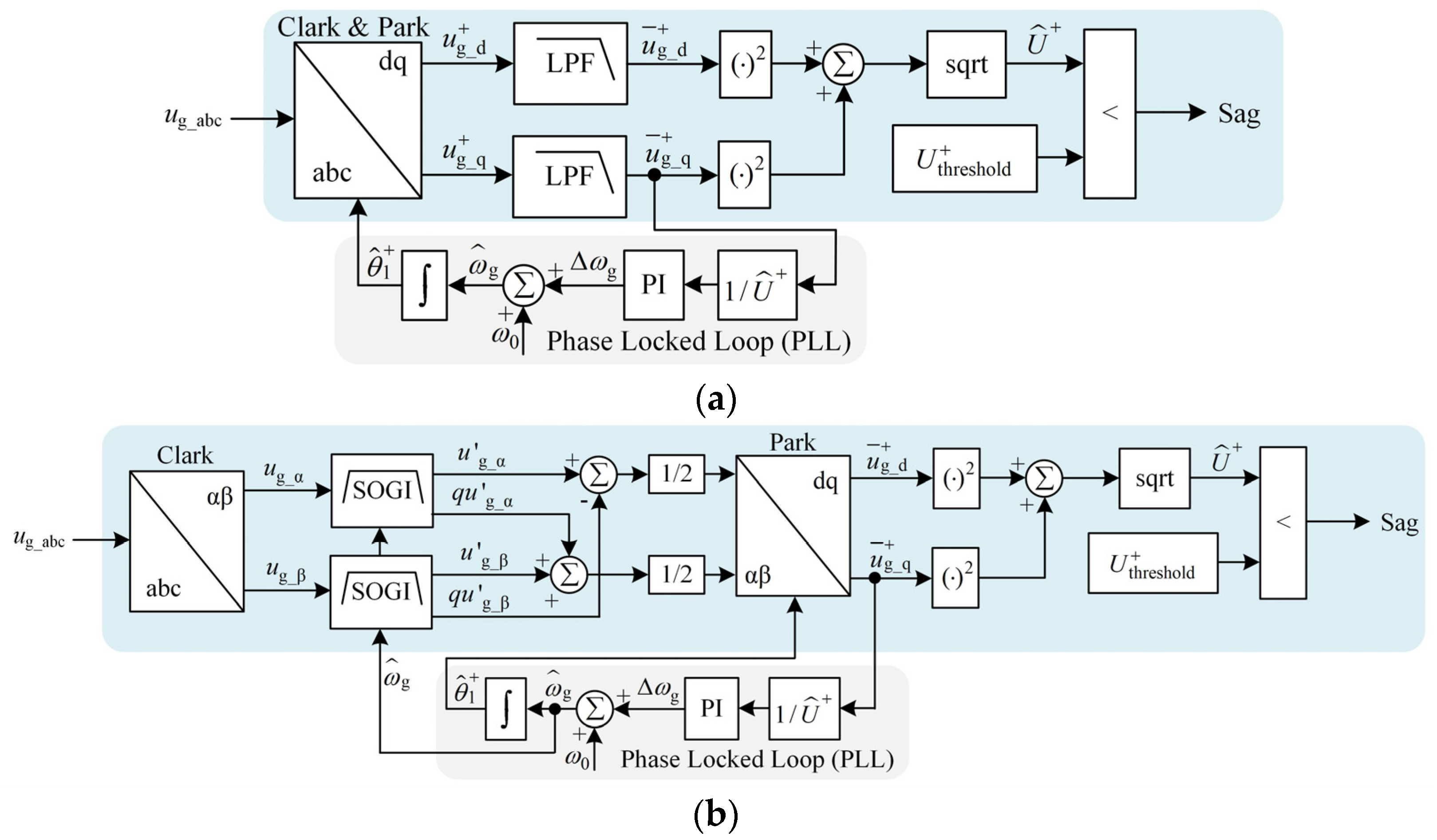
2. Voltage Sag and Traditional Detection Methods Based on SRF

The three primary factors that contribute to voltage sag in a three-phase and three-wire (3ph-3w) power system are short-circuit fault, induction motor starting, and lightning strike [41]. Short-circuit fault is by far the most significant factor. According to features, voltage sags caused by short-circuit faults can be separated into 7 categories (A to G) [42], as illustrated in Figure 2 [43]. Sag types D, F, and G is the derived type propagated by various types of transformers, whereas sag types A, B, C, and E stands for three-phase symmetrical short circuit, single-phase short circuit, phase-to-phase short circuit, and two-phase grounding short circuit, respectively.

Except for type A in Figure 2, the voltage sag types belong to unbalanced voltage sag. If harmonic disturbance is also taken into account, the three-phase grid voltage can be assumed as

$$\begin{array}{l}{u}_{\mathrm{g}\_\mathrm{a}}(t)={\displaystyle \sum _{h=1,3,5,7,\dots }\left[U_{\mathrm{h}}^{+}\cos \left(h{\omega }_{\mathrm{g}}t+{\phi }_{\mathrm{h}}^{+}\right)+U_{\mathrm{h}}^{-}\cos \left(h{\omega }_{\mathrm{g}}t+{\phi }_{\mathrm{h}}^{-}\right)\right]}\\ u_{\mathrm{g}\_\mathrm{b}}(t)={\displaystyle \sum _{h=1,3,5,7,\dots }\left[U_{\mathrm{h}}^{+}\cos \left(h{\omega }_{\mathrm{g}}t+{\phi }_{\mathrm{h}}^{+}-\frac{2\mathsf{\pi }}{3}\right)+U_{\mathrm{h}}^{-}\cos \left(h{\omega }_{\mathrm{g}}t+{\phi }_{\mathrm{h}}^{-}+\frac{2\mathsf{\pi }}{3}\right)\right]}\\ u_{\mathrm{g}\_\mathrm{c}}(t)={\displaystyle \sum _{h=1,3,5,7,\dots }\left[U_{\mathrm{h}}^{+}\cos \left(h{\omega }_{\mathrm{g}}t+{\phi }_{\mathrm{h}}^{+}+\frac{2\mathsf{\pi }}{3}\right)+U_{\mathrm{h}}^{-}\cos \left(h{\omega }_{\mathrm{g}}t+{\phi }_{\mathrm{h}}^{-}-\frac{2\mathsf{\pi }}{3}\right)\right]}\end{array}$$

(1)

where $U_{\mathrm{h}}^{+}$($U_{\mathrm{h}}^{-}$) and ${\phi }_{\mathrm{h}}^{+}$(${\phi }_{\mathrm{h}}^{-}$) represent the amplitude and the phase angle of the hth harmonic component of the positive-sequence (negative-sequence) of the grid voltage, respectively, and h = 1 represents the fundamental voltage. Furthermore, ω_g is the actual angular frequency of fundamental voltage of power grid.

Using Clark transformation [44], the three-phase grid voltage can be formulated as

$$\left[\begin{array}{l}{u}_{\mathrm{g}\_\mathsf{\alpha }}(t)\\ u_{\mathrm{g}\_\mathsf{\beta }}(t)\end{array}\right]={\mathit{T}}_{\mathsf{\alpha }\mathsf{\beta }}\left[\begin{array}{l}{u}_{\mathrm{g}\_\mathrm{a}}(t)\\ u_{\mathrm{g}\_\mathrm{b}}(t)\\ u_{\mathrm{g}\_\mathrm{c}}(t)\end{array}\right]=\left[\begin{array}{l}{\displaystyle \sum _{h=1,3,5,7,\dots }\left[U_{\mathrm{h}}^{+}\cos \left(h{\omega }_{\mathrm{g}}t+{\phi }_{\mathrm{h}}^{+}\right)+U_{\mathrm{h}}^{-}\cos \left(h{\omega }_{\mathrm{g}}t+{\phi }_{\mathrm{h}}^{-}\right)\right]}\\ {\displaystyle \sum _{h=1,3,5,7,\dots }\left[U_{\mathrm{h}}^{+}\sin \left(h{\omega }_{\mathrm{g}}t+{\phi }_{\mathrm{h}}^{+}\right)-U_{\mathrm{h}}^{-}\sin \left(h{\omega }_{\mathrm{g}}t+{\phi }_{\mathrm{h}}^{-}\right)\right]}\end{array}\right]$$

(2)

where

$${\mathit{T}}_{\mathsf{\alpha }\mathsf{\beta }}=\frac{2}{3}\left[\begin{array}{ccc}1& -\hspace{1em}\frac{1}{2}& -\hspace{1em}\frac{1}{2}\\ 0& \frac{\sqrt{3}}{2}& -\frac{\sqrt{3}}{2}\end{array}\right]$$

(3)

Applying Park transform [45] with the estimated fundamental positive-sequence phase angle ${\widehat{\theta }}_1^{+}$, the three-phase grid voltage in synchronous reference frame can be expressed as

$$\left[\begin{array}{l}{u}_{\mathrm{g}\_\mathrm{d}}^{+}(t)\\ u_{\mathrm{g}\_\mathrm{q}}^{+}(t)\end{array}\right]={\mathit{T}}_{\mathrm{dq}}^{+}\left[\begin{array}{l}{u}_{\mathrm{g}\_\mathsf{\alpha }}(t)\\ u_{\mathrm{g}\_\mathsf{\beta }}(t)\end{array}\right]=\left[\begin{array}{l}{\displaystyle \sum _{h=1,3,5,7,\dots }\left[U_{\mathrm{h}}^{+}\cos \left((h{\omega }_{\mathrm{g}}-{\widehat{\omega }}_{\mathrm{g}})t+({\phi }_{\mathrm{h}}^{+}-{\widehat{\phi }}_1^{+})\right)+U_{\mathrm{h}}^{-}\cos \left((h{\omega }_{\mathrm{g}}+{\widehat{\omega }}_{\mathrm{g}})t+({\phi }_{\mathrm{h}}^{-}+{\widehat{\phi }}_1^{+})\right)\right]}\\ {\displaystyle \sum _{h=1,3,5,7,\dots }\left[U_{\mathrm{h}}^{+}\sin \left((h{\omega }_{\mathrm{g}}-{\widehat{\omega }}_{\mathrm{g}})t+({\phi }_{\mathrm{h}}^{+}-{\widehat{\phi }}_1^{+})\right)-U_{\mathrm{h}}^{-}\sin \left((h{\omega }_{\mathrm{g}}+{\widehat{\omega }}_{\mathrm{g}})t+({\phi }_{\mathrm{h}}^{-}+{\widehat{\phi }}_1^{+})\right)\right]}\end{array}\right]$$

(4)

where

$${\mathit{T}}_{\mathrm{dq}}^{+}=\left[\begin{array}{cc}\cos {\widehat{\theta }}_1^{+}& \sin {\widehat{\theta }}_1^{+}\\ -\sin {\widehat{\theta }}_1^{+}& \cos {\widehat{\theta }}_1^{+}\end{array}\right]$$

(5)

Under a quasi-locked condition when the estimated angular frequency ${\widehat{\omega }}_{\mathrm{g}}$ is equal to ω_g, (4) can be approximated as

$$\left[\begin{array}{l}{u}_{\mathrm{g}\_\mathrm{d}}^{+}(t)\\ u_{\mathrm{g}\_\mathrm{q}}^{+}(t)\end{array}\right]\approx \left[\begin{array}{c}{\overline{u}}_{\mathrm{g}\_\mathrm{d}}^{+}(t)\\ {\overline{u}}_{\mathrm{g}\_\mathrm{q}}^{+}(t)\end{array}\right]+\left[\begin{array}{c}{\tilde{u}}_{\mathrm{g}\_\mathrm{d}}^{+}(t)\\ {\tilde{u}}_{\mathrm{g}\_\mathrm{q}}^{+}(t)\end{array}\right]$$

(6)

where

$$\left[\begin{array}{c}{\overline{u}}_{\mathrm{g}\_\mathrm{d}}^{+}(t)\\ {\overline{u}}_{\mathrm{g}\_\mathrm{q}}^{+}(t)\end{array}\right]=\left[\begin{array}{c}{U}_1^{+}\cos \left(\Delta {\phi }_1^{+}\right)\\ U_1^{+}\sin \left(\Delta {\phi }_1^{+}\right)\end{array}\right]\approx \left[\begin{array}{c}{U}_1^{+}\\ U_1^{+}·{\widehat{\theta }}_1^{+}\end{array}\right]$$

(7)

$$\begin{array}{l}\left[\begin{array}{c}{\tilde{u}}_{\mathrm{g}\_\mathrm{d}}^{+}(t)\\ {\tilde{u}}_{\mathrm{g}\_\mathrm{q}}^{+}(t)\end{array}\right]=\left[\begin{array}{l}{U}_1^{-}\cos \left((2{\omega }_{\mathrm{g}})t+({\phi }_{\mathrm{h}}^{-}+{\widehat{\phi }}_1^{+})\right)\\ -U_1^{-}\sin \left((2{\omega }_{\mathrm{g}})t+({\phi }_{\mathrm{h}}^{-}+{\widehat{\phi }}_1^{+})\right)\end{array}\right]+\\ \left[\begin{array}{l}{\displaystyle \sum _{h=3,5,7,\dots }\left[U_{\mathrm{h}}^{+}\cos \left(((h-1){\omega }_{\mathrm{g}})t+({\phi }_{\mathrm{h}}^{+}-{\widehat{\phi }}_1^{+})\right)+U_{\mathrm{h}}^{-}\cos \left(((h+1){\omega }_{\mathrm{g}})t+({\phi }_{\mathrm{h}}^{-}+{\widehat{\phi }}_1^{+})\right)\right]}\\ {\displaystyle \sum _{h=3,5,7,\dots }\left[U_{\mathrm{h}}^{+}\sin \left(((h-1){\omega }_{\mathrm{g}})t+({\phi }_{\mathrm{h}}^{+}-{\widehat{\phi }}_1^{+})\right)-U_{\mathrm{h}}^{-}\sin \left(((h+1){\omega }_{\mathrm{g}})t+({\phi }_{\mathrm{h}}^{-}+{\widehat{\phi }}_1^{+})\right)\right]}\end{array}\right]\end{array}$$

(8)

It is clear from Equations (7) and (8) that the numbers of positive-sequence or negative-sequence components of the hth harmonic will decrease or increase by 1 after Park transformation. For instance, the negative-sequence of the fundamental component will rise to 2nd-frequency one, while the positive-sequence of the 5th harmonic will be transformed to the 4th one, etc. Equation (8) can be simplified as

$$\left[\begin{array}{c}{\tilde{u}}_{\mathrm{g}\_\mathrm{d}}^{+}(t)\\ {\tilde{u}}_{\mathrm{g}\_\mathrm{q}}^{+}(t)\end{array}\right]=\left[\begin{array}{c}{f}_{\mathrm{d}}(2{\omega }_{\mathrm{g}},4{\omega }_{\mathrm{g}},6{\omega }_{\mathrm{g}},8{\omega }_{\mathrm{g}},\dots )\\ f_{\mathrm{q}}(2{\omega }_{\mathrm{g}},4{\omega }_{\mathrm{g}},6{\omega }_{\mathrm{g}},8{\omega }_{\mathrm{g}},\dots )\end{array}\right]$$

(9)

It can be seen that when asymmetric sag occurs with odd harmonics (3rd, 5th, 7th harmonic, etc.), the result of Park transformation includes even harmonics (2nd, 4th, 6th harmonic, etc.) in addition to the DC component corresponding to positive-sequence fundamental component. Traditional methods to calculate the voltage amplitude based on SRF are SRF-LPF and DSOGI-SRF, of which the structures are depicted in Figure 3. It should also be noted that 0.9 p.u. was selected as the threshold for detecting the sag event according to IEC 61000-4-30 and IEEE Std 1159-2019. In order to limit the influence of low-frequency harmonics after Park transformation on the calculation of the positive-sequence amplitude of fundamental wave, the cut-off frequency of LPF is usually tuned to be relatively low in SRF-LPF [32], which will result in a delay in the judgement of voltage sag. Owing to bandpass characteristics, DSOGI extracts of the fundamental positive-sequence component in αβ synchronous reference frame [36]. However, in order to filter out low-frequency harmonics before Park transformation, e.g., 3rd, 5th, or 7th harmonics, DSOGI generally needs to reduce the dynamic response performance.

In order to eliminate the influence of the low-frequency harmonic components of the power grid on voltage sag detection, this paper proposes a flexibly configurable fundamental or harmonic extraction algorithm (called SHEA) that can extract the selected harmonic component and suppress the influence of other harmonics, realizing the decoupling calculation of fundamental and harmonics of power grid voltage.

3. SHEA Principle and Performance Analysis

3.1. Mathematical Modelling of SHEA

The actual control system completes the calculation of the control algorithm in each discrete sampling period after sampling and holding, so the modeling and implementation of the proposed method will be based on the discrete domain rather than the ideal continuous domain. Considering the general situation, the measured voltage u(k) at the kth moment contains N harmonic components (0, 1,…, N−1), where the 0th harmonic refers to the DC component. Firstly, assuming that the rated fundamental frequency of u(k) is ω₀, the discrete state variable x_h(k) of the hth harmonic is constructed with a pair of orthogonal bases in αβ coordinate plane, as follows. Additionally, the linear combination of orthogonal bases x_h(k) can be used to represent vectors on any plane:

$${\mathit{x}}_{\mathrm{h}}(k)=\left(\begin{array}{l}{x}_{\mathrm{h}1}(k)\\ x_{\mathrm{h}2}(k)\end{array}\right)=\left(\begin{array}{c}\frac{\sqrt{2}}{2}{U}_{\mathrm{h}}\sin (h{\omega }_{0}k{T}_s+{\phi }_{\mathrm{h}}+\frac{\mathsf{\pi }}{4})\\ -\frac{\sqrt{2}}{2}{U}_{\mathrm{h}}\cos (h{\omega }_{0}k{T}_s+{\phi }_{\mathrm{h}}+\frac{\mathsf{\pi }}{4})\end{array}\right)$$

(10)

where T_s is the sampling period and U_h and φ_h are the AC RMS and phase angle of the hth harmonic, respectively. Using the discrete state variables of the hth harmonic, the expression of the hth harmonic u_h(k) to be extracted from the measured voltage u(k) can be written as

$${\mathit{u}}_{\mathrm{h}}(k)=\left(\begin{array}{cc}1& 1\end{array}\right){\mathit{x}}_{\mathrm{h}}(k)=U_{\mathrm{h}}\sin (h{\omega }_{0}k{T}_{\mathrm{s}}+{\phi }_{\mathrm{h}})$$

(11)

The expression of the discrete state variable x_h(k + 1) of the hth harmonic at (k + 1)th moment is

$$\begin{array}{l}{\mathit{x}}_{\mathrm{h}}(k+1)=\left(\begin{array}{l}{x}_{\mathrm{h}1}(k+1)\\ x_{\mathrm{h}2}(k+1)\end{array}\right)=\left(\begin{array}{c}\frac{\sqrt{2}}{2}{U}_{\mathrm{h}}\sin (h{\omega }_{0}k{T}_{\mathrm{s}}+{\phi }_{\mathrm{h}}+\frac{\mathsf{\pi }}{4}+h{\omega }_0{T}_{\mathrm{s}})\\ -\frac{\sqrt{2}}{2}{U}_{\mathrm{h}}\cos (h{\omega }_{0}k{T}_{\mathrm{s}}+{\phi }_{\mathrm{h}}+\frac{\mathsf{\pi }}{4}+h{\omega }_0{T}_{\mathrm{s}})\end{array}\right)\hspace{1em}\\ \hspace{1em}=\left(\begin{array}{cc}\cos (h{\omega }_0{T}_{\mathrm{s}})& -\sin (h{\omega }_0{T}_{\mathrm{s}})\\ \sin (h{\omega }_0{T}_{\mathrm{s}})& \cos (h{\omega }_0{T}_{\mathrm{s}})\end{array}\right)\left(\begin{array}{l}{x}_{\mathrm{h}1}(k)\\ x_{\mathrm{h}2}(k)\end{array}\right)={\mathit{S}}_{\mathrm{h}}·{\mathit{x}}_{\mathrm{h}}(k)\end{array}$$

(12)

where S_h is a second-order rotating transformation matrix of the hth harmonic and the state variable is extended to all N harmonic points as (13):

$$\mathit{x}(k)={\left(\begin{array}{ccc}{\mathit{x}}_0(k)& \cdots & {\mathit{x}}_{\mathrm{N}-1}(k)\end{array}\right)}^{{\rm T}}$$

(13)

Therefore, the state equation model of N harmonic is as follows:

$$\mathit{x}(k+1)=\left(\begin{array}{ccc}{\mathit{S}}_0& & \\ & \ddots & \\ & & {\mathit{S}}_{\mathrm{N}-1}\end{array}\right)\mathit{x}(k)=\mathit{S}·\mathit{x}(k)$$

(14)

where S is a 2N-order square matrix, and x(k) is a 2N-dimensional column vector. As can be observed, the state variable x(k) is not affected by the input voltage u(k), so the system performs uncontrolled. After neglecting the high-frequency component with small amplitude, the expression of u(k) can be written as

$$\mathit{u}(k)={\displaystyle \sum _{h=0}^{N-1}{\mathit{u}}_{\mathrm{h}}(k)}=\left(\begin{array}{ccc}\left(\begin{array}{cc}1& 1\end{array}\right)& \cdots & \left(\begin{array}{cc}1& 1\end{array}\right)\end{array}\right)\left(\begin{array}{c}{\mathit{x}}_0(k)\\ ⋮\\ {\mathit{x}}_{\mathrm{N}-1}(k)\end{array}\right)={\mathit{E}}_{1\times 2\mathrm{N}}·\mathit{x}(k)$$

(15)

where E_1×2N represents a matrix of dimension (1 × 2N) with all elements of 1.

After introducing the controllability factor µ associated with the input voltage u(k), Equation (15) can be rewritten as

$$\mu ·\mathit{u}(k)=\mu {\mathit{E}}_{1\times 2\mathrm{N}}·\mathit{x}(k)$$

(16)

Therefore, the equation of state model of the hth harmonic (Equation (12)) can be expressed as

$${\mathit{x}}_{\mathrm{h}}(k+1)={\mathit{S}}_{\mathrm{h}}·{\mathit{x}}_{\mathrm{h}}(k)-\mu {\mathit{E}}_{2\times 2\mathrm{N}}·\mathit{x}(k)+\mu {\mathit{E}}_{2\times 1}·\mathit{u}(k)$$

(17)

The state-space model for the hth harmonic extraction is

$$\{\begin{array}{l}{\mathit{x}}_{\mathrm{h}}(k+1)={\mathit{S}}_{\mathrm{h}}·{\mathit{x}}_{\mathrm{h}}(k)-\mu {\mathit{E}}_{2\times 2\mathrm{N}}·\mathit{x}(k)+\mu {\mathit{E}}_{2\times 1}·\mathit{u}(k)\\ {\mathit{y}}_{\mathrm{h}}(k)=\left(\begin{array}{cc}1& 1\end{array}\right){\mathit{x}}_{\mathrm{h}}(k)+\left(0\right)\mathit{u}(k)\end{array}$$

(18)

and the state-space model of all N harmonic extraction can be derived as

$$\{\begin{array}{l}\mathit{x}(k+1)=\left(\mathit{S}-\mu {\mathit{E}}_{2\mathrm{N}\times 2\mathrm{N}}\right)·\mathit{x}(k)+\mu {\mathit{E}}_{2\mathrm{N}\times 1}·\mathit{u}(k)\\ \mathit{y}(k)={\left(\begin{array}{ccc}\left(\begin{array}{cc}1& 1\end{array}\right)& & \\ & \ddots & \\ & & \left(\begin{array}{cc}1& 1\end{array}\right)\end{array}\right)}_{(\mathrm{N}\times 2\mathrm{N})}\mathit{x}(k)+{\left(\begin{array}{c}0\\ ⋮\\ 0\end{array}\right)}_{(\mathrm{N}\times 1)}\mathit{u}(k)\end{array}$$

(19)

Finally, the SHEA model considering N harmonic extraction is

$$\{\begin{array}{l}\mathit{x}(k+1)=\mathit{A}\mathit{x}(k)+\mathit{B}\mathit{u}(k)\\ \mathit{y}(k)=\mathit{C}\mathit{x}(k)+\mathit{D}\mathit{u}(k)\end{array}$$

(20)

The expressions for system matrix A, control matrix B, output matrix C, and direct transfer matrix D of the state-space model are shown in Equation (19). All the parametric matrices are time-independent constant–coefficient matrices, so the SHEA model is a linear time invariant (LTI) system.

Figure 4 is the amplitude–frequency curve of SHEA. When the number of selective extraction h is equal to 0, the gain of SHEA in the low frequency band is 0 dB with a dramatic negative gain at the even-frequency points, which indicates that SHEA can effectively extract the selected DC component and suppress the impacts of other harmonics at the same time. When h is equal to 2, SHEA has zero gain at the 2nd-frequency harmonic (100 Hz), with a great attenuation to other even-harmonic components. The other cases are similar; that is, SHEA can extract the selected harmonic and simultaneously suppress the negative effect of other harmonics, realizing the decoupling of the desired signal and the disturbed signal.

In order to achieve the detection of voltage sag, this paper mainly considers the case h = 0. Specifically, SHEA is placed after Park transformation (similar to the SRF-LPF structure in Figure 3a) to realize selective extraction of DC components and suppress even-harmonic interference (2nd, 4th, 6th harmonic, etc.). The details related to sag detection will be discussed in the next section.

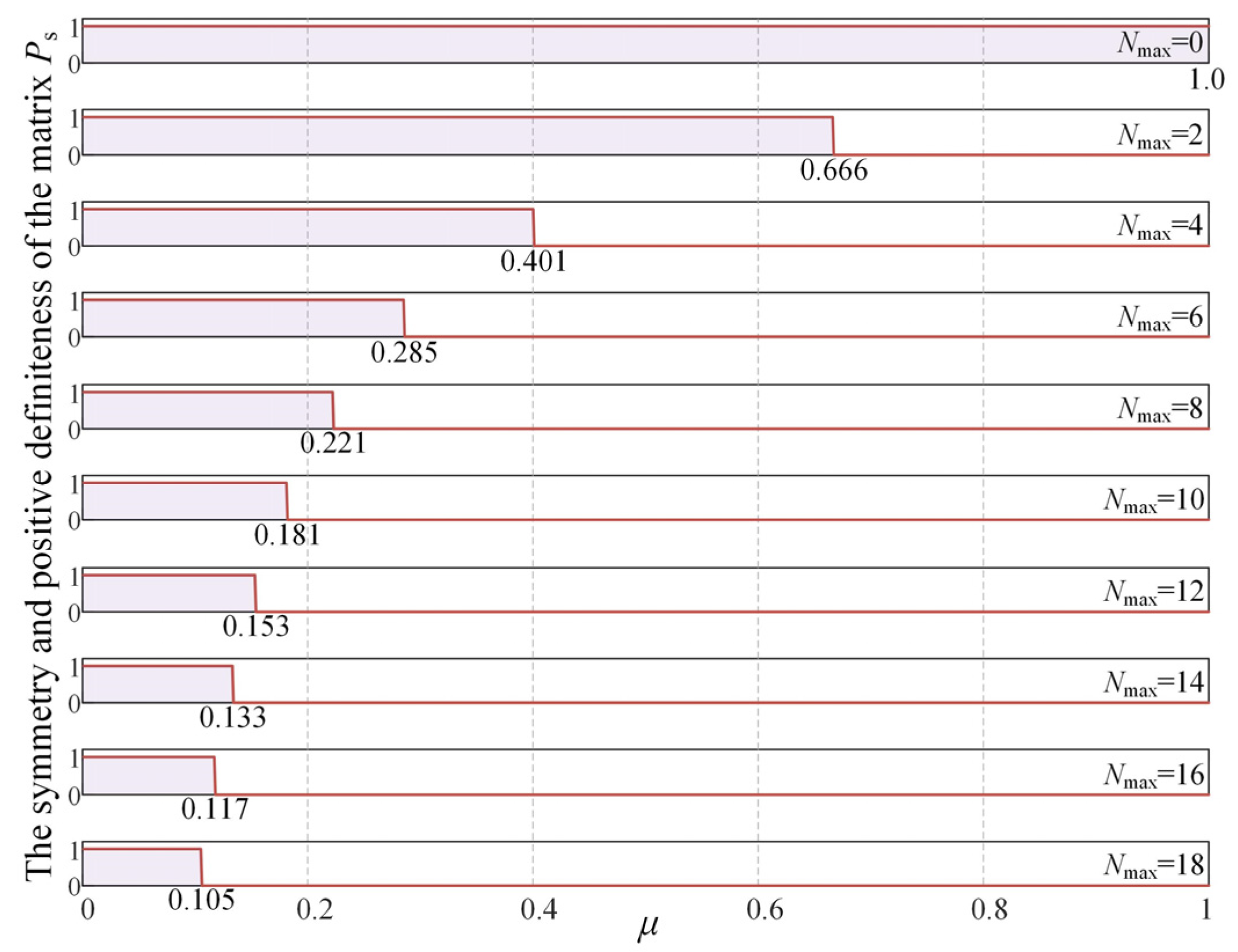
3.2. Controllability and Stability Analysis of SHEA

It is vital to theoretically analyze the controllability and stability of SHEA prior to application because they are prerequisite for proper operation.

3.2.1. Controllability Analysis

Firstly, the controllability of the system is analyzed. According to the control matrix B (Equation (19)) of the established state-space model, the influence extent of the state variable x(k) by the unbound input signal u(k) can be characterized by controllability factor μ. The discriminant criterion for the complete controllability of a LTI system [46,47] is that the controllability matrix P_c is a nonsingular matrix defined as

$${\mathit{P}}_{\mathrm{c}}=\left(\begin{array}{ccccc}\mathit{B}& \mathit{A}\mathit{B}& {\mathit{A}}^2\mathit{B}& \cdots & {\mathit{A}}^{\mathrm{N}-1}\mathit{B}\end{array}\right)$$

(21)

Therefore, the controllability of the system is determined by the system matrix A and the control matrix B. Specifically, for the certain sampling period T_s and fundamental frequency ω₀, matrix A and B are affected by the highest harmonic number N_max and controllability factor μ. Since the number of harmonics selectively extracted or eliminated by SHEA is 0, 2, 4, …, N_max, the controllability criterion related to matrix rank can be calculated as follows:

$$\mathrm{rank}({\mathit{P}}_{\mathrm{c}})=N_{\max }+2$$

(22)

When N_max is configured large, the system order is correspondingly high, and the calculation process of the analytical solution is laborious. Therefore, the parameter traversal approach is used to analyze the relationship between the numerical solution of the matrix rank and system parameters, as illustrated in Figure 5. The shaded area indicates that the controllability matrix P_c can achieve uninterrupted full rank, that is, the continuous controllable interval of SHEA. As can be observed, with the increase of N_max, μ will gradually decrease to ensure that the model is controllable. For example, when N_max ≤ 6, μ can be any value within (0,1), and the range of μ has been limited to (0.030,0.117) when N_max = 16. Additionally, when N_max = 18, the highest rank of the controllability matrix P_c is 19 (<20), which means that there is no μ capable of making P_c full rank. In other words, the system is uncontrolled. Consequently, the controllability of SHEA will decrease with the increase of the highest harmonic number N_max. To ensure that the SHEA system is always controllable, N_max in this paper is selected as 14 and the corresponding value range for parameter μ is (0,0.151).

3.2.2. Stability Analysis

Lyapunov’s analysis methodology [48,49] is used to evaluate the stability of SHEA model, which is a LTI discrete system. This is because Lyapunov is more direct for the analysis of a state-space model compared with the classical algebraic criterion, Nyquist criterion, eigenvalue criterion, etc., whether the original system is linear or nonlinear. Firstly, the Lyapunov function of the SHEA model is constructed as a quadratic function, as follows:

$$V(\mathit{x}(k))={\mathit{x}}^{\mathrm{T}}(k){\mathit{P}}_{\mathrm{s}}\mathit{x}(k)$$

(23)

Combined with Equation (20) of the SHEA model, the corresponding Lyapunov algebraic equation can be obtained as

$${\mathit{A}}^{\mathrm{T}}{\mathit{P}}_{\mathrm{s}}\mathit{A}-{\mathit{P}}_{\mathrm{s}}=-\mathit{Q}$$

(24)

The sufficient and necessary condition for the asymptotic stability of the system is that given a positive definite symmetric matrix Q, there exists a positive definite symmetric matrix P_s, which makes the algebraic Equation (24) hold. According to (24), the stability of the system is determined by the system matrix A, and for the system with specific sampling period T_s and fundamental frequency ω₀, matrix A is influenced by the highest harmonic number N_max and parameter μ.

Since the number of harmonics selectively extracted or eliminated by SHEA is 0, 2, 4, …, N_max, the positive definite symmetric matrix Q can take the unit square matrix I of order (N_max + 2). If the calculated matrix P_s is a real symmetric matrix by numerical analysis, sufficient and necessary conditions for P_s to be positive is that all the eigenvalues of the matrix are positive. Figure 6 illustrates the relationship between the symmetric positive definiteness of the stability-related matrix P_s and parameter μ under various N_max, where the shaded region represents that P_s has a symmetric positive definite property, that is, the asymptotic stability interval of the system. In order to ensure the stability of SHEA, the range of μ will gradually decrease as N_max increases. For instance, when N_max = 1, μ can be specified as any value within (0,1) while when N_max = 18, the range narrows to (0,0.105). Therefore, the asymptotic stability of the SHEA model will decline with the increase of the highest harmonic number N_max. In this paper, the selected N_max is 14, and the range of μ is (0,0.133).

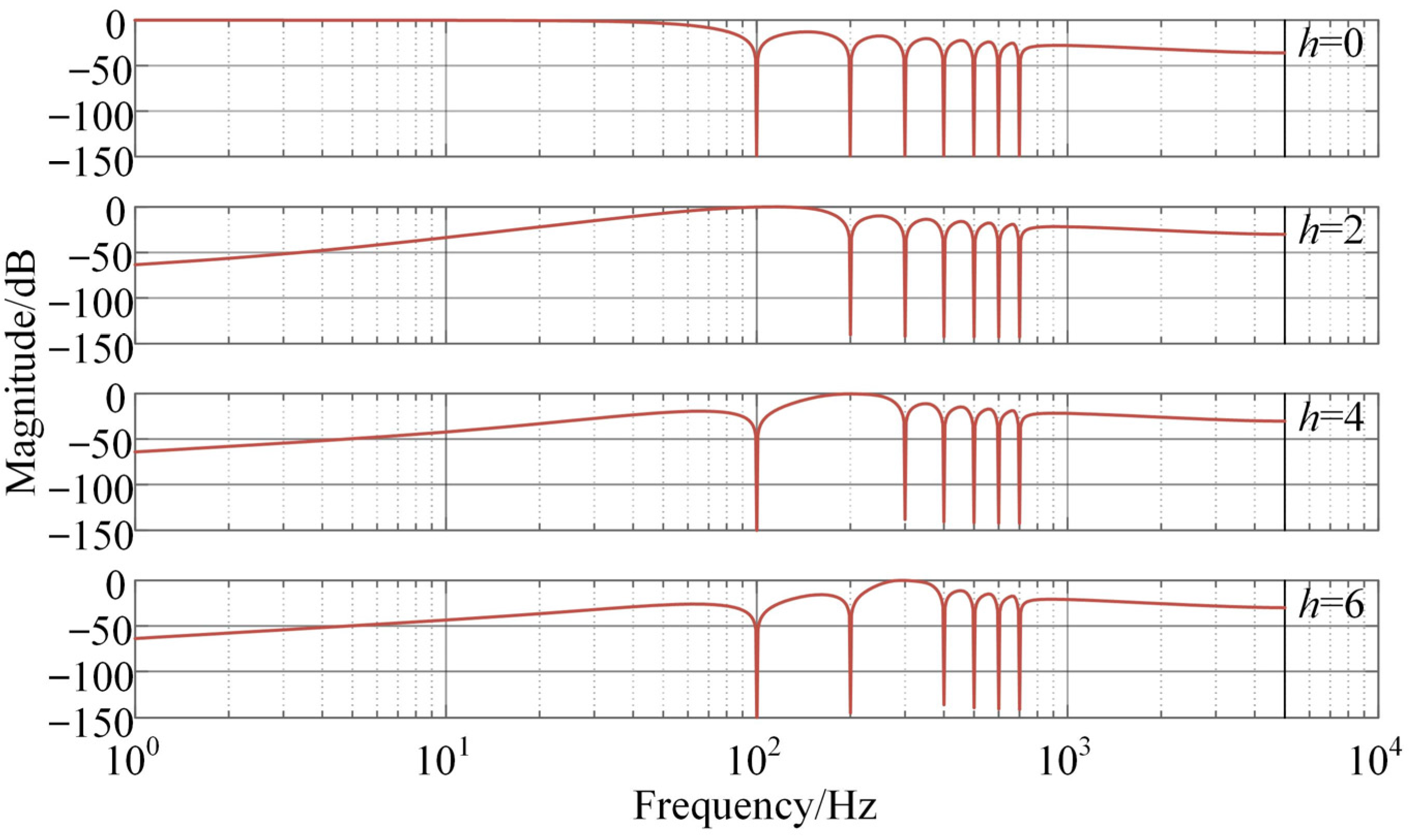
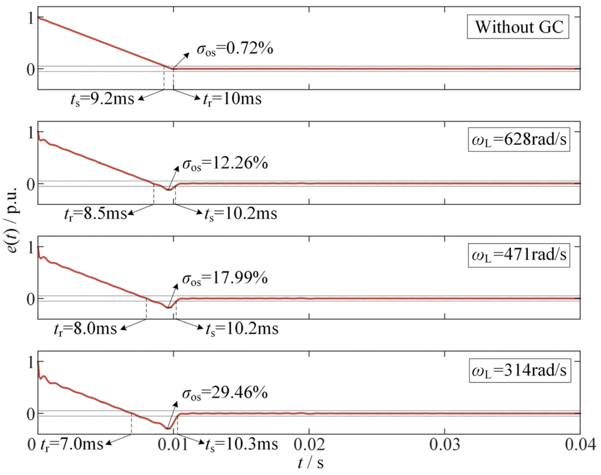
3.3. Performance Evaluation of SHEA

When the SHEA model satisfies the controllability and stability conditions, the system performance of the model needs to be investigated thoroughly, which consists of dynamic and steady-state performance. Since SHEA selectively extracts the DC component after Park transformation in the disturbed signal, the dynamic performance of SHEA in the time domain can be characterized by the overshoot (σ_os) and the convergence time (t_s) of the response error e(t) to a unit step. Additionally, the steady-state performance can be quantified by the steady-state error (e_ss) after convergence. It should be noted that t_s is defined as the time required for e(t) to reach and maintain within ±2%, while σ_os is defined as the percentage of the overshoot peak of e(t) relative to e_ss, which can be expressed as (25):

$$e_{\mathrm{ss}}={\left[\mathit{u}(t)-{\mathit{y}}_0(t)\right]}_{t\to \infty }$$

(25)

Figure 7 depicts the convergence curve of SHEA error under different N_max and μ. It can be seen that e_ss can always converge to zero, regardless of the parameters. Therefore, its steady-state performance is excellent. The increase of N_max scarcely affects the value of σ_os and t_s, that is, the dynamic property is almost irrelevant to the system’s order. However, the effect of μ on the dynamic performance of SHEA is not monotonic. With the increase of μ, the convergence time (t_s) tends to decrease and subsequently increase, which is brought on by the overshoot (σ_os) that is from scratch and progressively raised.

According to Figure 7, when N_max = 14, the dynamic performance of SHEA is optimal when μ is 0.024. Additionally, the convergence time (t_s) is 9.2ms, while the overshoot (σ_os) is only 0.72%. Combined with the above analysis, the SHEA model under this parameter is controllable and stable, so μ in this paper is set as 0.024.

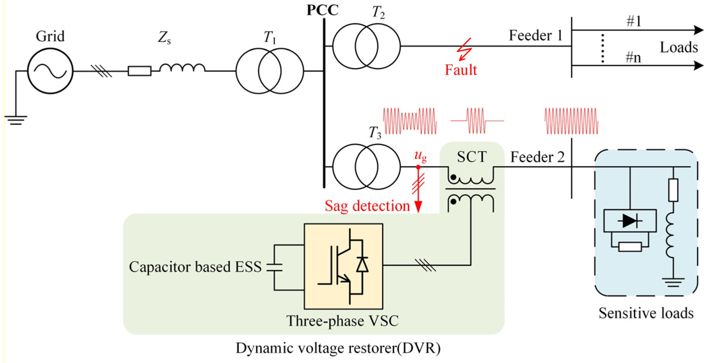
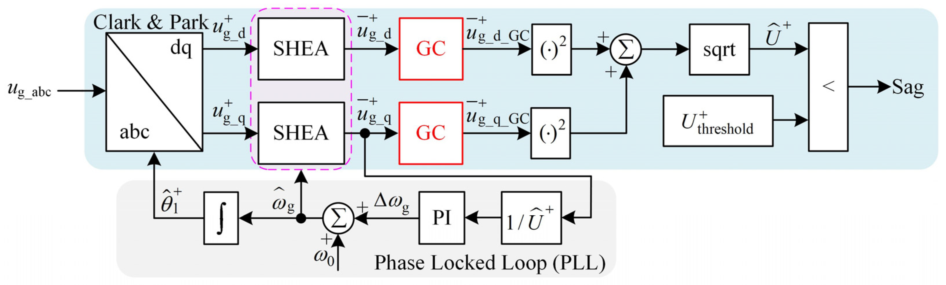
4. A Novel Voltage Sag Detection Method Based on SHEA and Its Optimization

As stated previously, the application of SHEA in voltage sag detection can be flexible in that it can be connected either after or before Park transformation. For the former, SHEA extracts the DC component and suppresses even-harmonic interference (2nd, 4th, 6th harmonic, etc.) simultaneously, similar to the SRF-LPF structure in Figure 3a. For the latter, it extracts the fundamental positive-sequence component and eliminates odd-harmonic disturbance (3rd, 5th, 7th harmonic, etc.), like the DSOGI-SRF structure in Figure 3b. To facilitate the subsequent optimization analysis, SHEA is placed after Park transformation in this paper. The voltage sag detection method based on SHEA is shown in Figure 8. The threshold for sag event is also defined as 0.9 p.u. Phase-locked loop (PLL) is integrated into the proposed method for frequency adaptation. In addition, the gain compensator (GC) in the figure is employed to improve the dynamic performance of SHEA, which will be discussed below.

SHEA realized the suppression of low- and medium-frequency harmonics that have a significant impact on the accuracy of voltage detection, which is vividly shown in Figure 4 (h = 0). Therefore, the gains of low- and medium-frequency bands can be considered to be compensated to enhance the dynamic performance. The proposed gain compensator (GC) consists of one zero and one pole. The discretized expression using bilinear transformation is as follows:

$$\mathrm{GC}(z)={\frac{1+s/{\omega }_{\mathrm{L}}}{1+s/{\omega }_{\mathrm{H}}}|}_{s=\frac{2}{T_{\mathrm{s}}}\frac{z-1}{z+1}}=\frac{(1+\frac{2}{{\omega }_{\mathrm{L}}{T}_{\mathrm{s}}})z+(1-\frac{2}{{\omega }_{\mathrm{L}}{T}_{\mathrm{s}}})}{(1+\frac{2}{{\omega }_{\mathrm{H}}{T}_{\mathrm{s}}})z+(1-\frac{2}{{\omega }_{\mathrm{H}}{T}_{\mathrm{s}}})}$$

(26)

where ω_L and ω_H represent the transition angle frequency of the zero and the pole, respectively. The selection of ω_H is determined according to the highest harmonic number N_max of SHEA, which can retain a certain high-frequency attenuation ability of the algorithm. Additionally, ω_L determines the gain compensation ability of GC for the low- and medium-frequency bands of SHEA.

The Bode diagram of SHEA after GC compensation at various ω_L is depicted in Figure 9. The gain of the envelope of SHEA with GC in the low- and medium-frequency bands will be higher along with the decrease of ω_L; in other words, the loss of the side-lobe gain around DC signal will be smaller, which means that the dynamic response speed of the system will be better theoretically.

However, the performance is not directly correlated with the GC’s compensation capacity of gain. The dynamic performance of SHEA with GC should meet the demand of voltage sag detection. For instance, short rise time (t_r) is needed to detect the occurrence of voltage sag promptly; short convergence time (t_s) ensures the quick calculation of the accurate voltage compensation instructions for DVR; and small overshoot (σ_os) implies an accurate sag judgment and a low probability of incorrect identification.

Figure 10 shows the convergence curve of error (e(t)) for SHEA with GC under unit step with different ω_L. As can be seen, with ω_L decreases, the rise time (t_r) decreases dramatically (here, t_r is defined as the moment when e(t) decreases to zero for the first time). However, the decrease in the rise time is at the expense of system overshoot. For example, when ω_L = 314 rad/s, t_r, decreased to 7.0 ms from 10.0 ms, but σ_os increased to 29.46% from 0.72% after compensation. In addition, the convergence time is hardly affected by the zero-related parameter ω_L, and SHEA with GC can always converge around 10 ms.

Under the premise that the accuracy of sag judgment is guaranteed, the rapidity of the algorithm can be optimized according to Figure 10. The zero corresponding to σ_os = 15% is chosen as the parameter for GC: ω_L = 540 rad/s, with t_r = 8.2 ms.

5. Simulation Results

The performance of voltage sag detection based on SHEA with GC was verified in a MATLAB/Simulink simulation toolbox and compared with traditional detection methods. The voltage sag detection method needs to adapt to the nonideal power grid environment, including three-phase unbalance, phase variation, frequency drift, low-frequency harmonic disturbance, etc. The detailed simulation parameters are summarized in

Table 1. The main parameters.

Parameter	Value
Rated grid line voltage (Ug_line)	380 V (1.0 p.u.)
Rated frequency (f0)	50 Hz
Symmetrical sag depth (Udepth1)	0.4 p.u.
Asymmetrical sag depth (Udepth2)	0.2 p.u.
Variation of frequency (fvariation)	+5 Hz
Variation of phase angle (θvariation)	−20°
Background harmonic distortion	0.05 p.u. 5th positive-sequence harmonic 0.05 p.u. 7th negative-sequence harmonic
Injected harmonic disturbance	0.10 p.u. 3rd positive-sequence harmonic 0.05 p.u. 5th positive-sequence harmonic 0.01 p.u. 5 kHz noise
Sampling frequency (fs)	10 kHz
Threshold for sag judgment (U+threshold)	0.9 p.u.

.

The adaptability and robustness of the method is confirmed by complex operating conditions. Several grid conditions are considered in this paper as follows:

(1)

Symmetrical voltage sag with U_depth1 happens in a three-phase power grid.

(2)

The three-phase power grid undergoes an asymmetrical sag of type C (as shown in Figure 2) with U_depth2.

(3)

Symmetrical voltage sag with U_depth1 occurs accompanied by phase variation θ_variation.

(4)

Symmetrical voltage sag with U_depth1 occurs accompanied by frequency drift of f_variation.

(5)

Symmetrical voltage sag with U_depth1 occurs injected with harmonic disturbance, which is given in Table 1.

(6)

The three-phase power grid experiences an asymmetrical sag of type C accompanied by phase variation of θ_variation, frequency drift of f_variation and harmonic disturbance.

Moreover, aside from SRF-LPF and DSOGI-SRF, the numerical matrix in [16], SRF-RMS in [35], and GDFT [27] are taken into account to make a comparison with the proposed detection method. It should be noted that the feasibility and effectiveness of methods can be validated by judge time t_j and convergence time t_s of zero steady-state error. The judge time t_j is the interval between the sag event occurrence and the moment when the method reaches the threshold (0.9 p.u.).

5.1. Comparison with SRF-LPF and DSOGI-SRF

The performance of the proposed method is compared with that of the traditional methods SRF-LPF and DSOGI-SRF in the cases of six sag conditions.

The results of symmetrical sag (grid condition 1) are shown in Figure 11a. Among the three schemes, SHEA with GC minimizes the interval (t_j) to identify the sag occurrence as 1.0 ms compared with SRF-LPF (2.9 ms) and DSOGI-SRF (1.9 ms). Although the 2% convergence time (t_s) of SHEA with GC (10.4 ms) is a little longer than that of SRF-LPF (9.3 ms), the convergence time around 10 ms is reasonable since the system overshoot (σ_os) of SHEA with GC is in exchange for the judgment speed, which is consistent with the error convergence analysis in Figure 10.

In Figure 11b, the results of the asymmetric sag (grid condition 2) are displayed. It takes 5.4 ms, 4.5 ms, and 3.8 ms for SRF-LPF, DSOGI-SRF, and SHEA with GC respectively to detect the occurrence of voltage sag. Additionally, asymmetric voltage sag will induce a fundamental negative-sequence component, so that SRF-LPF without fundamental negative-sequence suppression ability has poor accuracy with steady-state ripple around 10%Vp-p. In comparison, the fundamental negative-sequence component can be effectively eliminated by both DSOGI-SRF and SHEA with GC, and the convergence is finished at 7.4 ms and 5.5 ms, respectively. Specifically, SHEA with GC performs better in both dynamic state and steady state.

The results for phase variation (grid condition 3) and frequency drift (grid condition 4) are shown in Figure 11c and Figure 11d, respectively. SHEA with GC needs only 1.0 ms to detect the occurrence of voltage sag caused by additional phase jump, while the other two methods, SRF-LPF and DSOGI-SRF, need 2.8 ms and 1.6 ms, respectively. The case of frequency drift is analogous, where SRF-LPF, DSOGI-SRF, and SHEA with GC take 2.9 ms, 1.5 ms, and 0.8 ms, respectively. The convergence times t_s in these two grid conditions are close to those in grid condition 1. The difference is that the time t_s is influenced by the background harmonic distortion.

Figure 11e depicts the results of harmonic interference (grid condition 5). SHEA with GC takes only 1.3 ms to determine the occurrence of voltage sag, while the traditional method takes 3.3 ms and 2.3 ms as a benchmark. In addition, due to the insufficient attenuation of SRF-LPF and DSOGI-SRF for low-frequency harmonics, there are low-frequency oscillations after stabilization, and the ripple amplitudes are 5% Vp-p and 7% Vp-p, respectively. In comparison, SHEA with GC completes zero-error convergence after 10.2 ms, showing a strong ability to resist the harmonics.

In the face of complex operating conditions such as asymmetric sag, phase variation, frequency drift, and harmonic disturbance (grid condition 6 in Figure 11f), the dynamic and steady performance of SHEA with GC is outstanding compared with conventional techniques, especially when it comes to judging speed, convergence time, and steady-state accuracy. SRF-LPF and DSOGI-SRF require 6.3 ms and 6.7 ms to determine the occurrence of sag, whereas SHEA with GC requires only 4.5 ms. The traditional approaches suffer from low-frequency oscillation following quasi-convergence, which is associated with negative-sequence and harmonic components, while SHEA with GC has almost no fluctuation after convergence at 12.3 ms and the steady-state accuracy is relatively high.

5.2. Comparison with Other Methods

The performance of the proposed method is compared with that of other methods such as numerical matrix, SRF-RMS, and GDFT. The test cases are selected as symmetrical sag (grid condition 1) and harmonic interference (grid condition 5).

The results of symmetrical sag (grid condition 1) are shown in Figure 12a. The method of numerical matrix consumes 1.1 ms to detect the occurrence of the sag event, while it only takes 3.7 ms to finish the convergence for the voltage calculation after a significant oscillation. Furthermore, the proposed SHEA with GC minimizes the interval (t_j) to identify the sag occurrence as 1.0 ms, in contrast with SRF-RMS (2.6 ms), GDFT (2.2 ms). Compared with the numerical matrix, the 2% convergence time (t_s) for the other three methods are 9.6 ms, 6.9 ms, and 10.4 ms. Although the dynamic response speed of the numerical matrix is outstanding among the four schemes, the robustness is relatively poor, illustrated in Figure 12b (grid condition 5). When encountering high-frequency noise, which has been neglected in the design process, the correct results will not be obtained by numerical matrix. That is, the sag event will be missing. Separately, the other three methods, SRF-RMS, GDFT, and SHEA with GC, spend, respectively, 3.0 ms, 2.6 ms, and 1.3 ms to determine the occurrence of sag. In comparison with the results in Figure 12, SRF-RMS and GDFT have longer judge times (t_j) and faster convergence speeds. In other words, these two methods have a strong robustness but a slow detection speed. Additionally, numerical matrix is not suitable for nonideal grid conditions even though it has a relatively good dynamic speed, and the proposed SHEA with GC performs well in both dynamic and steady-state performance.

5.3. Reliability Discussion

In order to confirm the reliability of the proposed method, a shallow sag (0.95 p.u.) with frequency drift (+5 Hz) and large harmonic distortion (0.10 p.u. 5th positive-sequence harmonic and 0.10 p.u. 7th negative-sequence harmonic) is considered to be used as a false sag event.

The results of five detection methods for shallow sag event are shown in Figure 13. SRF-LPF, SRF-RMS, and SHEA with GC will not identify this event as a true sag event: The false margins, defined as the difference between the lowest detection value and the value (0.9 p.u.), are 0.04 p.u., 0.038 p.u., 0.015 p.u., respectively. Conversely, DSOGI-SRF and GDFT will recognize the shallow sag event as a real sag event as a result of the large harmonic distortion. Separately, numerical matrix will produce an incorrect judgement due to the oscillation related to its sensitivity to the nonideal conditions.

False positive events will trigger the DVR into compensation mode when no real voltage sag has occurred. The proposed SHEA with GC method has a relatively fast detection speed (Figure 11 and Figure 12) and an acceptable false margin (Figure 13); that is, the method makes a reasonable compromise between sensitivity and robustness. Furthermore, the dynamic or steady-state performance of different voltage sag detection methods for different nonideal grid conditions is summarized in

Table 2. The performance of the different voltage detection methods.

Grid Conditions	Performance Metrics	SRF-LPF [32]	DSOGI-SRF [36]	Numerical Matrix [16]	SRF-RMS [35]	GDFT [25]	Proposed Method
Symmetrical sag	Judge time tj (0.9 p.u.)	2.9 ms	1.9 ms	1.1 ms	2.6 ms	2.2 ms	1.0 ms
	Convergence time ts (2%)	9.3 ms	12.0 ms	3.7 ms	9.6 ms	6.9 ms	10.4 ms
Asymmetrical sag	Judge time tj (0.9 p.u.)	5.4 ms	4.5 ms	1.2 ms	5.2 ms	3.5 ms	3.8 ms
	Convergence time ts (2%)	10% Vp-p ripple	7.4 ms	3.0 ms	7.5 ms	9.3 ms	5.5 ms
Symmetrical sag with phase variation	Judge time tj (0.9 p.u.)	2.8 ms	1.6 ms	1.1 ms	2.3 ms	1.7 ms	1.0 ms
	Convergence time ts (2%)	9.2 ms	28.6 ms	3.8 ms	9.5 ms	15.2 ms	13.3 ms
Symmetrical sag with frequency drift	Judge time tj (0.9 p.u.)	2.9 ms	1.5 ms	1.1 ms	2.5 ms	1.9 ms	0.8 ms
	Convergence time ts (2%)	9.3 ms	24.4 ms	25% Vp-p ripple	9.4 ms	11.9 ms	10.2 ms
Symmetrical sag with harmonic interference	Judge time tj (0.9 p.u.)	3.3 ms	2.3 ms	missing	3.0 ms	2.6 ms	1.3 ms
	Convergence time ts (2%)	5% Vp-p ripple	7% Vp-p ripple	—	9.3 ms	6.5 ms	10.2 ms
Asymmetrical sag with comprehensive disturbance	Judge time tj (0.9 p.u.)	6.3 ms	6.7 ms	missing	5.8 ms	2.2 ms	4.5 ms
	Convergence time ts (2%)	7% Vp-p ripple	7% Vp-p ripple	—	3.2% Vp-p ripple	14.2 ms	12.3 ms
Shallow symmetrical sag	False margin (relative to 0.9 p.u.)	0.04 p.u.	false	false	0.038 p.u.	false	0.015 p.u.

. Additionally, the judge time of GDFT under asymmetrical sag is smaller because it is based on the detection of each phase rather than a three-phase positive-sequence component.

6. Conclusions

Traditional voltage sag detection methods are unable to quickly and accurately identify the occurrence of voltage sag in harmonically disturbed nonideal power grids. In this paper, a novel selective harmonic extraction method (SHEA) is proposed, and a parameter configuration method based on controllability analysis, stability analysis, and convergence analysis is given. Additionally, the dynamic response speed of the sag detection based on SHEA is optimized with a well-designed gain compensator (GC). The simulation results show that compared with the traditional sag detection methods, the method based on SHEA with GC has good dynamic and steady-state performance as well as excellent disturbance immunity, which can meet requirements under nonideal grid conditions. The proposed sag detection method can provide theoretical support for the rapid start-up and high-precision compensation of power quality equipment such as DVR.

References

1. Khergade, A.V.; Satputaley, R.J.; Borghate, V.B.; Raghava, B. Harmonics Reduction of Adjustable Speed Drive Using Transistor Clamped H-Bridge Inverter Based DVR With Enhanced Capacitor Voltage Balancing. IEEE Trans. Ind. Appl. 2020, 56, 6744–6755. [Google Scholar] [CrossRef]
2. Emerging Power Quality Problems and State-of-the-Art Solutions. IEEE Trans. Ind. Electron. 2017, 64, 761–763. [CrossRef] [Green Version]
3. Moghassemi, A.; Padmanaban, S. Dynamic Voltage Restorer (DVR): A Comprehensive Review of Topologies, Power Converters, Control Methods, and Modified Configurations. Energies 2020, 13, 4152. [Google Scholar] [CrossRef]
4. Ghodsi, M.; Barakati, S.M.; Guerrero, J.M.; Vasquez, J.C. Dynamic Voltage Restore Based on Switched-Capacitor Multilevel Inverter with Ability to Compensate for Voltage Drop, Harmonics, and Unbalancing Simultaneously. Electr. Power Syst. Res. 2022, 207, 107826. [Google Scholar] [CrossRef]
5. Abas, N.; Dilshad, S.; Khalid, A.; Saleem, M.S.; Khan, N. Power Quality Improvement Using Dynamic Voltage Restorer. IEEE Access 2020, 8, 164325–164339. [Google Scholar] [CrossRef]
6. Khergade, A.; Satputaley, R.; Patro, S.K. Investigation of Voltage Sags Effects on ASD and Mitigation Using ESRF Theory-Based DVR. IEEE Trans. Power Deliv. 2021, 36, 3752–3764. [Google Scholar] [CrossRef]
7. Tu, C.; Guo, Q.; Jiang, F.; Wang, H.; Shuai, Z. A Comprehensive Study to Mitigate Voltage Sags and Phase Jumps Using a Dynamic Voltage Restorer. IEEE J. Emerg. Sel. Top. Power Electron. 2020, 8, 1490–1502. [Google Scholar] [CrossRef]
8. Zhang, H.; Xiao, G.; Lu, Z.; Chai, Y. Reduce Response Time of Single-Phase Dynamic Voltage Restorer (DVR) in a Wide Range of Operating Conditions for Practical Application. IEEE J. Emerg. Sel. Top. Power Electron. 2022, 10, 2101–2113. [Google Scholar] [CrossRef]
9. Li, Z.; Guo, X.; Wang, Z.; Yang, R.; Zhao, J.; Chen, G. An Optimal Zero-Sequence Voltage Injection Strategy for DVR Under Asymmetric Sag. IEEE J. Emerg. Sel. Top. Power Electron. 2022, 10, 2595–2607. [Google Scholar] [CrossRef]
10. Koroglu, T.; Tan, A.; Savrun, M.M.; Cuma, M.U.; Bayindir, K.C.; Tumay, M. Implementation of a Novel Hybrid UPQC Topology Endowed With an Isolated Bidirectional DC–DC Converter at DC Link. IEEE J. Emerg. Sel. Top. Power Electron. 2020, 8, 2733–2746. [Google Scholar] [CrossRef]
11. Soomro, A.H.; Larik, A.S.; Mahar, M.A.; Sahito, A.A.; Soomro, A.M.; Kaloi, G.S. Dynamic Voltage Restorer—A Comprehensive Review. Energy Rep. 2021, 7, 6786–6805. [Google Scholar] [CrossRef]
12. Chawda, G.S.; Shaik, A.G.; Mahela, O.P.; Padmanaban, S.; Holm-Nielsen, J.B. Comprehensive Review of Distributed FACTS Control Algorithms for Power Quality Enhancement in Utility Grid With Renewable Energy Penetration. IEEE Access 2020, 8, 107614–107634. [Google Scholar] [CrossRef]
13. Pal, R.; Gupta, S. Topologies and Control Strategies Implicated in Dynamic Voltage Restorer (DVR) for Power Quality Improvement. Iran. J. Sci. Technol. Trans. Electr. Eng. 2020, 44, 581–603. [Google Scholar] [CrossRef]
14. Molla, E.M.; Kuo, C.-C. Voltage Quality Enhancement of Grid-Integrated PV System Using Battery-Based Dynamic Voltage Restorer. Energies 2020, 13, 5742. [Google Scholar] [CrossRef]
15. Chen, G.; Zhang, L.; Wang, R.; Zhang, L.; Cai, X. A Novel SPLL and Voltage Sag Detection Based on LES Filters and Improved Instantaneous Symmetrical Components Method. IEEE Trans. Power Electron. 2015, 30, 1177–1188. [Google Scholar] [CrossRef]
16. Fitzer, C.; Barnes, M.; Green, P. Voltage Sag Detection Technique for a Dynamic Voltage Restorer. IEEE Trans. Ind. Appl. 2004, 40, 203–212. [Google Scholar] [CrossRef]
17. Florio, A.; Mariscotti, A.; Mazzucchelli, M. Voltage Sag Detection Based on Rectified Voltage Processing. IEEE Trans. Power Deliv. 2004, 19, 1962–1967. [Google Scholar] [CrossRef]
18. Chen, C.-I.; Chen, Y.-C.; Chen, C.-H.; Chang, Y.-R. Voltage Regulation Using Recurrent Wavelet Fuzzy Neural Network-Based Dynamic Voltage Restorer. Energies 2020, 13, 6242. [Google Scholar] [CrossRef]
19. Chang, G.W.; Chen, C.-I. Performance Evaluation of Voltage Sag Detection Methods. In Proceedings of the IEEE PES General Meeting, Minneapolis, MN, USA, 25–29 July 2010; pp. 1–6. [Google Scholar]
20. Gupta, N.; Seethalekshmi, K. Artificial Neural Network and Synchrosqueezing Wavelet Transform Based Control of Power Quality Events in Distributed System Integrated with Distributed Generation Sources. Int. Trans. Electr. Energy Syst. 2021, 31, e12824. [Google Scholar] [CrossRef]
21. Katić, V.A.; Stanisavljević, A.M. Smart Detection of Voltage Dips Using Voltage Harmonics Footprint. IEEE Trans. Ind. Appl. 2018, 54, 5331–5342. [Google Scholar] [CrossRef]
22. Stanisavljević, A.M.; Katić, V.A. Magnitude of Voltage Sags Prediction Based on the Harmonic Footprint for Application in DG Control System. IEEE Trans. Ind. Electron. 2019, 66, 8902–8912. [Google Scholar] [CrossRef]
23. Bagheri, A.; Mardaneh, M.; Rajaei, A.; Rahideh, A. Detection of Grid Voltage Fundamental and Harmonic Components Using Kalman Filter and Generalized Averaging Method. IEEE Trans. Power Electron. 2016, 31, 1064–1073. [Google Scholar] [CrossRef]
24. Li, J.; Yang, Y.; Lin, H.; Teng, Z.; Zhang, F.; Xu, Y. A Voltage Sag Detection Method Based on Modified S Transform With Digital Prolate Spheroidal Window. IEEE Trans. Power Deliv. 2021, 36, 997–1006. [Google Scholar] [CrossRef]
25. Liu, H.; Hu, H.; Chen, H.; Zhang, L.; Xing, Y. Fast and Flexible Selective Harmonic Extraction Methods Based on the Generalized Discrete Fourier Transform. IEEE Trans. Power Electron. 2018, 33, 3484–3496. [Google Scholar] [CrossRef]
26. Sridharan, K.; Babu, B.C. Accurate Phase Detection System Using Modified SGDFT-Based PLL for Three-Phase Grid-Interactive Power Converter During Interharmonic Conditions. IEEE Trans. Instrum. Meas. 2022, 71, 9000311. [Google Scholar] [CrossRef]
27. Neves, F.A.S.; de Souza, H.E.P.; Bradaschia, F.; Cavalcanti, M.C.; Rizo, M.; Rodriguez, F.J. A Space-Vector Discrete Fourier Transform for Unbalanced and Distorted Three-Phase Signals. IEEE Trans. Ind. Electron. 2010, 57, 2858–2867. [Google Scholar] [CrossRef]
28. Wang, Y.F.; Li, Y.W. Three-Phase Cascaded Delayed Signal Cancellation PLL for Fast Selective Harmonic Detection. IEEE Trans. Ind. Electron. 2013, 60, 1452–1463. [Google Scholar] [CrossRef]
29. Golestan, S.; Ramezani, M.; Guerrero, J.M.; Freijedo, F.D.; Monfared, M. Moving Average Filter Based Phase-Locked Loops: Performance Analysis and Design Guidelines. IEEE Trans. Power Electron. 2014, 29, 2750–2763. [Google Scholar] [CrossRef] [Green Version]
30. Taiwo, O.P.; Tiako, R.; Davidson, I.E. Voltage Unbalance Mitigation and Voltage Profile Enhancement in Secondary Distribution System Using Dynamic Voltage Restorer. Int. J. Eng. Res. Afr. 2018, 34, 81–101. [Google Scholar] [CrossRef]
31. Golestan, S.; Monfared, M.; Freijedo, F.D. Design-Oriented Study of Advanced Synchronous Reference Frame Phase-Locked Loops. IEEE Trans. Power Electron. 2013, 28, 765–778. [Google Scholar] [CrossRef]
32. Sillapawicharn, Y.; Kumsuwan, Y. Dual Low Pass Filter-Based Voltage Sag Detection for Voltage Sag Compensator under Distorted Grid Voltages. In Proceedings of the 2014 International Electrical Engineering Congress (iEECON), Chonburi, Thailand, 19–21 March 2014; pp. 1–4. [Google Scholar]
33. Golestan, S.; Guerrero, J.M.; Vasquez, J.C. A Robust and Fast Synchronization Technique for Adverse Grid Conditions. IEEE Trans. Ind. Electron. 2017, 64, 3188–3194. [Google Scholar] [CrossRef]
34. Kumsuwan, Y.; Sillapawicharn, Y. A Fast Synchronously Rotating Reference Frame-Based Voltage Sag Detection under Practical Grid Voltages for Voltage Sag Compensation Systems. In Proceedings of the 6th IET International Conference on Power Electronics, Machines and Drives (PEMD 2012), Bristol, UK, 27–29 March 2012; pp. 1–5. [Google Scholar]
35. Khoshkbar Sadigh, A.; Smedley, K.M. Fast and Precise Voltage Sag Detection Method for Dynamic Voltage Restorer (DVR) Application. Electr. Power Syst. Res. 2016, 130, 192–207. [Google Scholar] [CrossRef]
36. Xu, J.; Qian, H.; Hu, Y.; Bian, S.; Xie, S. Overview of SOGI-Based Single-Phase Phase-Locked Loops for Grid Synchronization Under Complex Grid Conditions. IEEE Access 2021, 9, 39275–39291. [Google Scholar] [CrossRef]
37. Dehghani Arani, Z.; Taher, S.A.; Ghasemi, A.; Shahidehpour, M. Application of Multi-Resonator Notch Frequency Control for Tracking the Frequency in Low Inertia Microgrids Under Distorted Grid Conditions. IEEE Trans. Smart Grid 2019, 10, 337–349. [Google Scholar] [CrossRef]
38. Rodríguez, P.; Luna, A.; Candela, I.; Mujal, R.; Teodorescu, R.; Blaabjerg, F. Multiresonant Frequency-Locked Loop for Grid Synchronization of Power Converters Under Distorted Grid Conditions. IEEE Trans. Ind. Electron. 2011, 58, 127–138. [Google Scholar] [CrossRef] [Green Version]
39. Luo, W.; Wei, D. A Frequency-Adaptive Improved Moving-Average-Filter-Based Quasi-Type-1 PLL for Adverse Grid Conditions. IEEE Access 2020, 8, 54145–54153. [Google Scholar] [CrossRef]
40. Roldán-Pérez, J.; García-Cerrada, A.; Ochoa-Giménez, M.; Zamora-Macho, J.L. Delayed-Signal-Cancellation-Based Sag Detector for a Dynamic Voltage Restorer in Distorted Grids. IEEE Trans. Sustain. Energy 2019, 10, 2015–2027. [Google Scholar] [CrossRef]
41. Alam, M.R.; Muttaqi, K.M.; Bouzerdoum, A. Characterizing Voltage Sags and Swells Using Three-Phase Voltage Ellipse Parameters. IEEE Trans. Ind. Appl. 2015, 51, 2780–2790. [Google Scholar] [CrossRef]
42. Bollen, M.H.J. Voltage Recovery after Unbalanced and Balanced Voltage Dips in Three-Phase Systems. IEEE Trans. Power Deliv. 2003, 18, 1376–1381. [Google Scholar] [CrossRef]
43. Ignatova, V.; Granjon, P.; Bacha, S. Space Vector Method for Voltage Dips and Swells Analysis. IEEE Trans. Power Deliv. 2009, 24, 2054–2061. [Google Scholar] [CrossRef] [Green Version]
44. Zou, Y.; Zhang, L.; Xing, Y.; Zhang, Z.; Zhao, H.; Ge, H. Generalized Clarke Transformation and Enhanced Dual-Loop Control Scheme for Three-Phase PWM Converters Under the Unbalanced Utility Grid. IEEE Trans. Power Electron. 2022, 37, 8935–8947. [Google Scholar] [CrossRef]
45. Islam, M.Z.; Reza, M.S.; Hossain, M.M.; Ciobotaru, M. Three-Phase PLL Based on Adaptive Clarke Transform Under Unbalanced Condition. IEEE J. Emerg. Sel. Top. Ind. Electron. 2022, 3, 382–387. [Google Scholar] [CrossRef]
46. Hu, Z.; Zhang, B.; Deng, W. Feasibility Study on One Cycle Control for PWM Switched Converters. In Proceedings of the 2004 IEEE 35th Annual Power Electronics Specialists Conference (IEEE Cat. No.04CH37551), Aachen, Germany, 20–25 June 2004; Volume 5, pp. 3359–3365. [Google Scholar]
47. Li, X.; Qu, L.; Ren, W.; Zhang, C.; Liu, S. Controllability of the Three-Phase Inverters Based on Switched Linear System Model. In Proceedings of the 2016 IEEE International Conference on Industrial Technology (ICIT), Taipei, Taiwan, 14–17 March 2016; pp. 287–292. [Google Scholar]
48. Yu, J.; Cheng, M.; Gao, D.; Gu, Y.; Yu, J. A Lyapunov Stability Theory-Based Control Method for Three-Level Shunt Active Power Filter. In Proceedings of the 2016 35th Chinese Control Conference (CCC), Chengdu, China, 27–29 July 2016; pp. 8683–8687. [Google Scholar]
49. Li, L.; Yang, H.; Guo, W.; Liu, Y. Analysis and Application of Lyapunov-Based Stable Control of the Single-Phase Shunt Active Power Filter. In Proceedings of the 2012 Asia-Pacific Power and Energy Engineering Conference, Shanghai, China, 27–29 March 2012; pp. 1–4. [Google Scholar]
Figure 1. Schematic of DVR.
Energies 15 05560 g001
Figure 2. The seven basic voltage sag types of the distribution network.
Energies 15 05560 g002
Figure 3. Traditional voltage sag detection methods based on SRF. (a) SRF-LPF; (b) DSOGI-SRF.
Energies 15 05560 g003
Figure 4. The amplitude–frequency curves of SHEA for different harmonic extractions.
Energies 15 05560 g004
Figure 5. The relationship between the rank of controllability matrix Pc and controllability factor μ under various Nmax.
Energies 15 05560 g005
Figure 6. The relationships between symmetric positive definiteness of the stability-related matrix Ps and parameter μ under various Nmax.
Energies 15 05560 g006
Figure 7. The relationships between the convergence curve of error e(t) and parameter μ under various Nmax.
Energies 15 05560 g007
Figure 8. The proposed voltage sag detection method based on SHEA.
Energies 15 05560 g008
Figure 9. Bode diagram of SHEA with GC with different zero-related parameters ωL.
Energies 15 05560 g009
Figure 10. Convergence curves of SHEA error with GC under unit steps with different zero-related parameters ωL.
Energies 15 05560 g010
Figure 11. The results for different voltage detection methods (SRF-LPF, DSOGI-SRF, SHEA with GC) under different working conditions: (a) symmetrical sag; (b) asymmetrical sag; (c) symmetrical sag with phase variation; (d) symmetrical sag with frequency drift; (e) symmetrical sag with low-frequency harmonic interference and high-frequency noise; (f) asymmetrical sag with comprehensive disturbance.
Energies 15 05560 g011
Figure 12. The results of different voltage detection methods (numerical matrix, SRF-RMS, GDFT, SHEA with GC) under different working conditions: (a) symmetrical sag; (b) symmetrical sag with high-frequency noise.
Energies 15 05560 g012
Figure 13. The results of different voltage detection methods in case of shallow sag events.
Energies 15 05560 g013