Deep-Learning Based Fault Events Analysis in Power Systems

Abstract

The identification of fault types and their locations is crucial for power system protection/operation when a fault occurs in the lines. In general, this involves a human-in-the-loop analysis to capture the transient voltage and current signals using a common format for transient data exchange for power systems (COMTRADE) file. Then, protection engineers can identify the fault types and the line locations after the incident. This paper proposes intelligent and novel methods of faulty line and location detection based on convolutional neural networks in the power system. The three-phase fault information contained in the COMTRADE file is converted to an image file and extracted adaptively by the proposed CNN, which is trained by a large number of images under various kinds of fault conditions and factors. A 500 kV power system is simulated to generate different types of electromagnetic fault transients. The test results show that the proposed CNN-based analyzer can classify the fault types and locations under various conditions and reduce the fault analysis efforts.

1. Introduction

Transmission lines are one of the vital components of power systems. The transmission system’s safety and protection are the primary concerns and challenging tasks to ensure the power system’s stability and reliability for seamless functioning and avoidance of any significant discrepancies [1]. Faults in power transmission lines can occur for many different reasons, e.g., short circuit, momentary tree contact, bird or other animal contact, lightning strike, earthquake, conductor clashing, and corrosion of equipment. Some of them are within human control, whereas some are naturally occurring. Once protective relays detect a fault, they must clear the fault in a timely manner [2,3].Even though there are many reasons for the occurrence of faults, tasks to find fault location and types (as a post-fault analysis) are still major concerns. By reducing the time of post-fault analysis, the faulted system can be maintained faster by reducing the restoration time, and this could reduce the failure costs. To enhance the resiliency and reliability of power system operation, the need for a fast, effective, and efficient fault type and location classification is becoming more and more necessary. The works of [4,5] proposed a conception of fault-location observability and a new fault-location scheme for transmission networks based on synchronized phasor measurement units (PMUs). In order to locate any fault in the power system, the deterministic and stochastic algorithms for placing a minimum number of PMUs in a power system were proposed in [6].

The tasks of fault type and location classification can be achieved by three steps: (1) importing transient fault data, (2) conducting pre-data processing for the appropriate algorithms, and (3) analyzing the fault data. The pre-data processing used could be S-transform, wavelet transform, or Fast Fourier Transform (FFT) to convert the fault signals of three-phase voltages and currents. The analysis of the fault data can be studied in different ways, e.g., a machine learning algorithm and a waveform-based correlation coefficient. There are several papers already published by various researchers, including the applications of machine learning and deep neural networks for classification and location of power system faults.

Moreover, these fault techniques have been categorized according to several different criteria and aspects, namely model-based approaches, knowledge-based methods, and data-driven approaches, when judgments are made based on the analysis and interpretation of numerical data rather than on observation or personal experience [7]. A data-driven strategy ensures that ideas and solutions are backed by verifiable facts rather than assumptions and personal experience. Machine learning methods to describe the fault analysis, particularly the applications of decision trees, support vector machines, and k-nearest neighbors (k-NN), have been proposed to classify the faults [8,9]. They showed that computational complexity to process the high-dimensional data and reduction techniques to reconstruct the data are required. However, the data reduction brings a risk of loss of information by lowering the dimensions, and the accuracy of the results is compromised. In Ref. [10], the authors propose a solution to extract features of PV cells based on the thermal image process and use the SVM algorithm to compare the results. A technique based on the fusion of time-domain descriptors (FTDD) is presented by the author in [11] to distinguish PQ disturbances from a typical pure sinusoidal signal. The effectiveness of the suggested strategy is then examined using multiclass SVM and Naive Bayes (NB) classifiers

The work of [3] identifies and categorizes various open-circuit fault types in power distribution systems, and the Modified Multi-Class Support Vector Machines (MMC-SVM) technique was proposed. The simulation results demonstrate the proposed machine learning model’s efficacy, and robustness [12].

The authors of [13] showed deep neural networks for power system fault analysis using pattern classification. The input fault features based on an artificial neural network (ANN) have been proposed to identify the location [14]. A probabilistic neural network with wavelet transformation is discussed in order to identify the fault types [15], but it is vulnerable to discrepancies in the input data. The work of [16] used unsupervised feature learning with sparse convolutional encoders to distinguish the fault types.

A fault prediction application of machine learning algorithms could improve the resiliency of the power transmission system. For instance, if a fault is triggered by abnormal power system operations (e.g., voltage instability issue or line-overloading problems), the machine learning model can be trained with abnormal data and predict the power system fault.

Both artificial neural network (ANN) and convolution neural network (CNN) models are machine learning models that are applied in many fields. Artificial neural networks (ANNs) are a group of non-linear statistical models and learning algorithms that have developed and evolved to mimic the behavior of connected neurons in organic neural systems. On the other hand, the convolutional neural network (CNN) model is an image recognition and classification model. Features are extracted from the image input when a CNN is used in network training. When thousands of features need to be extracted, CNN is appropriate. CNN organizes these features on its own rather than measuring each one individually. When using ANN, two-dimensional images must be translated into one-dimensional vectors, so image classification tasks become more challenging. This rapidly increases the number of trainable parameters, and increasing the number of trainable parameters necessitates more storage and processing capability.

A classification algorithm using convolutional neural networks (CNNs) with different sampling frequencies is proposed in [17]. Wavelet transform has been used to extract fault harmonics for the input of CNNs, but data generalization issues impact the classification decisions and the accuracy of the results in [18]. In deep neural networks, CNNs become an effective method for image classification and are used as building blocks for ResNet [19] and VGG Net [20]. CNNs are able to classify a large number of image databases from ImageNet [21]. There are different convolutional layers, pooling layers, and fully connected layers that are used to extract the essential features of the data from the images and classify them using supervised learning. In Ref. [22], the authors proposed a fault classifier based on a convolutional neural network and wavelet packet analysis. The authors of [23] successfully proposed classification based on CNN with raw input to improve the accuracy of transmission line faults.

However, applications of image classification for power systems in fault classification and line location identification have not been proposed, and extracting effective features and choosing appropriate classifiers have not been studied yet. Furthermore, the accuracy and efficiency of the detection results are not enough for practical implementation [24].

Therefore, this paper proposes CNN models for fault classification and line location identification under various power system conditions. In the proposed methods, a comprehensive system that preprocesses the data from the current signals has been successfully implemented. These continuous signals are plotted onto a graph using novel techniques to introduce graphical images of various power system faults.

The proposed CNN models are based on graphical images of power system faults. Simulation results show that the proposed CNN models can classify the fault type and line location very accurately. The contributions of our work are summarized as follows:

• An automated COMTRADE file analysis for fault type and location identification has been proposed using a testbed.
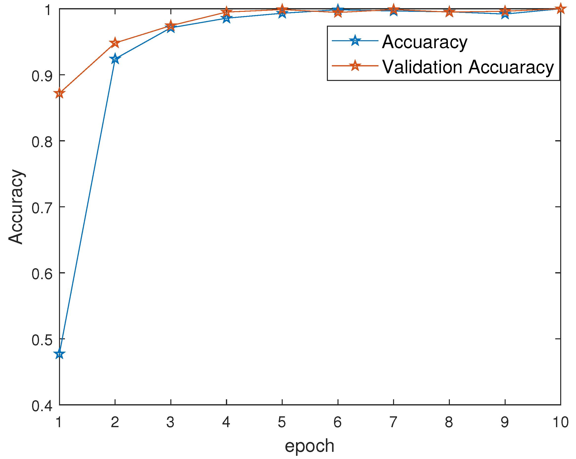
• A novel coloring method for the input of the proposed CNN model has been designed. The proposed CNN demonstrates the effectiveness for fault type and location classification with 99.9% classification accuracy. This is because the proposed CNN has the advantage of extracting features based on graphical images of power system faults.
• The proposed CNN model was tested with various kinds of transient fault data. The test results prove that the proposed method can be used to classify and detect fault types and transmission lines under various conditions of power systems.

2. Fault Analysis in Power Systems

Protective intelligent electronic devices (IEDs) monitor digitally sampled power system measurements and use protection schemes using digital signal processing algorithms to identify and detect faults or abnormal conditions in power systems. Once the IEDs detect a fault within the coordinated protection area, they can send a trip signal to the corresponding circuit breakers and clear the fault by opening the breakers. During this process, the IEDs generate the digitized transient fault data using the COMTRADE (common format for transient data exchange for power systems) format [25]. The format of the COMTRADE file is an IEEE standard (i.e., IEEE C37.111-2013) and refers to the recorded and stored transient power system disturbances (e.g., voltage, current, power, and frequency) that are generated by IEDs at electrical substations for analyzing system events [26]. The following equation shows an example of the ASCII data file format of a COMTRADE file.

$$\begin{array}{c}\hfill n,timestamp,A_1,A_2,\dots A_m,D_1,D_2,\dots D_k,\end{array}$$

(1)

where the first and second columns contain the sample number and the time stamp for the data, respectively, whereas the third and fourth sets of columns show the data values that represent analog information and the data for the status channels, respectively. Hence, the example below shows sample data that have three analog and three status values.

$$\begin{array}{c}\hfill 1,0,-993,1204,101,0,0,0<CR/LF>,\end{array}$$

(2)

where CR/LF is used to mark a line break in a COTRADE file. A COMTRADE file can be downloaded and viewed by various analysis tools from different manufacturers. The analyzed COMTRADE file can then show useful information related to the power system disturbance. Furthermore, COMTRADE files from multiple IEDs at different locations of substations can be collected to perform more sophisticated forensic analysis of large-scale power disturbance events (e.g., blackouts) to identify the root cause of the system disturbance, improve system protection engineers’ knowledge, and guide future system fault mitigation strategies. Usually, the generated COMTRADE file is analyzed and studied by protection engineers manually or through software platforms. This process could take up to several of hours or days to identify the cause of the system disturbance. Therefore, this paper proposes a fully automated system transient analysis tool by using a deep neural network to analyze the COMTRADE file and identify the system disturbance, e.g., fault type and location.

3. Proposed CNN Model for Fault Type and Location Classification

In this section, a CNN model for fault type and location classification is proposed. After generating the COMTRADE files for the training data, this model enables automatic COMTRADE file extraction and locates the faulted line and type. Figure 1 shows a block diagram that contains the data flow of the proposed algorithm. The data preprocessing module reduces the COMTRADE file information (e.g., three cycles of pre-disturbance, during the fault, and two cycles of post-fault) to minimize the dataset. Then it applies the coloring method so that all transient fault data are normalized and transformed into three-color-scale images to enhance the detection accuracy rate. The generated images are used as the CNN input for fault type and location classification in power systems. More details will be explained in the following subsections.

3.1. Data Preprocessing—Reduction

A total of ten different types of faults are generated in each transmission line for the training data. For instance, a substation with two transmission lines will generate 20 different classes, as shown in

Table 1. Input parameters for training and testing.

Model	Line Impedance			Bus Voltage (p.u.)				Fault Resistance (ohm)	Fault Location (miles from the SS#1)
	R (ohm/km)	L (mH/km)	C ($\mathsf{\mu }$f/km)	SS1	SS2	SS3	SS4
Network training	R1:0.012 R0:0.386	L1:0.933 L0:4.126	C1:0.012 C0:0.007	1.01	0.99	1.02	1.02	0.001, 0.1, 5, 20	20∼80
Model testing (different fault distance)	R1:0.012 R0:0.386	L1:0.933 L0:4.126	C1:0.012 C0:0.007	1.01	0.99	1.02	1.02	0.01, 0.3, 10, 15	10∼20, 80∼90

and

Table 2. Types of power system faults.

Type of Faults/Fault Line Location (Class Index)	Line 1 (0)	Line 2 (1)
	SLG-A $\left(0\right)$,	SLG-A $\left(10\right)$,
Single line to ground (class index)	SLG-B $\left(1\right)$,	SLG-B $\left(11\right)$,
	SLG-C $\left(2\right)$,	SLG-C $\left(12\right)$,
	DLG-AB $\left(3\right)$,	DLG-AB $\left(13\right)$,
Double line to ground (class index)	DLG-BC $\left(4\right)$,	DLG-BC $\left(14\right)$,
	DLG-AC $\left(5\right)$,	DLG-AC $\left(15\right)$,
	DLL-AB $\left(6\right)$,	DLL-AB $\left(16\right)$,
Double line to line (class index)	DLL-BC $\left(7\right)$,	DLL-BC $\left(17\right)$,
	DLL-AC $\left(8\right)$,	DLL-AC $\left(18\right)$,
Triple line to (class index)	TLG-ABC $\left(9\right)$	TLG-ABC $\left(19\right)$

. The simulated power system fault event contains a sampling frequency of 8 kHz and a pre-disturbance length of 1 s. A 500 kV power system simulation model is used to create fault event data and formatted to conform with the COMTRADE standard. The three-phase analog voltage and current signals are included in the generated event. Then, the COMTRADE data are reduced to show more details of pre-disturbance, fault, and post-fault information. Figure 2 shows the three-phase voltage, and current raw data that are extracted and reduced by the data preprocessing module. These graphs contain eight cycles overall, where the first three cycles of the data/graph represent the changes in the current values before the fault has occurred (pre-disturbance), the next three cycles represent the changes in the current data during the fault, and the last two cycles represent the data when there is an assertive action taken to neutralize the fault. In this case, the circuit breaker opened and cleared the fault. These generated files are our dataset for training, validating, and testing the proposed CNN model. There are twenty classes of faults and two classes for transmission lines. Each line has ten different types of faults, as follows: single line to ground faults (SLG-A, B, C), double lines to ground faults (DLG-AB, BC, AC), double linea to line faults (DLL-AB, BC, AC), and triple lines to ground fault (TLG-ABC). During the training process, 1000 image files per class are collected and produce a total of 20,000 images for the 20 classes.

3.2. Data Preprocessing—Coloring Method

As shown in Figure 2, multiple COMTRADE files are generated with different types of faults (Table 2). After reducing the COMTRADE data, the current-signal data points are plotted as a graph for representation that can visually identify the fault types and locations. This could help CNN and enhance the detection rate during the training process. A novel coloring method has been adopted to plot these graphs. An area graph is used for plotting the current signal values. This technique increases the spread of the graph, where the graph contains three-phase voltage and current values $V_a$, $V_b$, $V_c$ and $I_a$, $I_b$, $I_c$. Each phase is colored with a different color palette of RGB. For instance, red for the a phase, green for the b phase, and blue for eth c phase. This approach was developed to enhance the feature extraction capability of the proposed CNN for image classification. As the network will learn what it is fed, giving it changes in voltage and current as colored areas can make it more efficiently classify the task at hand. The novel coloring techniques have found much use for improving the color space mapping of the actual images. Initially, when mapping the COMTRADE data file onto the graphs, the data can be plotted using line graphs, as shown in Figure 2. However, when area graphs are used for plotting the data, a great deal of white space can be covered with meaningful color information about the image. This can be used by CNNs for processing the classification task. Initially, the line graphs were abundant in white space, dominating the entire information, and there is a possibility of obtaining sparse values while trying to process by the CNN model. Hence, the novel coloring method has been implemented. Figure 3 shows how the proposed CNN views the image for classifying the input image into the required class. Therefore, the proposed CNN was able to obtain higher availability of image-based fault transient information and make better decisions.

3.3. CNN Model

CNN models have been implemented for classifying various fault types and line locations, respectively. Figure 4 shows the structure of the proposed CNN for fault types, which contains an input layer, convolutional layers, max pooling, fully connected layers, and a softmax layer. The inputs for the proposed model are colored graphs of size $590\times 690\times 3$, where width and height are $590\times 690$ pixels and depth is 3 for RGB channels. The coloring images are used for fault types and location classification. Features for the input image are directly extracted and mapped to form new feature maps by using the convolution layer [27].

At each convolution unit, the ReLU activation function is used [28], which is expressed as

$$\begin{array}{c}\hfill f\left(z^l\right)=\left\{\begin{array}{c}{z}^l,\mathrm{if}{z}^l\ge 0,\hfill \\ 0,\mathrm{otherwise},\hfill \end{array}\right.\end{array}$$

(3)

where $z^l$ is element of outputs in the lth convolutional layer. In addition, the max pooling layer plays an important role in decreasing the spatial size of features and parameters, which help to reduce the computational complexity in the model but still preserve important features [29]. In our proposed approach, max pooling layers are used between convolutional layers in order to reduce the input data size. After the convolutional and max pooling layers, the flatten function is used to convert all the pooled feature maps into a single-dimensional vector that is connected to the fully connected layer. The fully connected layer compiles the features extracted by the previous layers to form the new feature map. Finally, the softmax layer is used after the fully connected layer. At the output layer, the output for M classes is calculated as

$$\begin{array}{c}\hfill \mathbf{z}={[z_1,\dots ,z_M]}^T=\sigma \left(\mathbf{h}\right),\end{array}$$

(4)

where $z_m$ is the predicted fault type in the m-th category of the M classes; $\sigma \left(\mathbf{h}\right)$ is the softmax function; and the output of the last fully connected layer, $\mathbf{h}={[h_1,\dots .,h_M]}^T$, is defined as

$$\begin{array}{c}\hfill z_m={\left[\sigma \right(\mathbf{h}\left)\right]}_m=\frac{e^{h_m}}{{\sum }_{j=1}^M{e}^{h_j}}.\end{array}$$

(5)

The parameters of the CNN model are learned so as to minimize the loss function through training dataset V. A cross entropy between prediction and target is used as a loss function for the ith training sample and is calculated as

$$\begin{array}{c}\hfill Loss\left({\mathbf{z}}^{\left(i\right)}\right)=-\sum _{m=1}^M{t}_m^{\left(i\right)}log\left(z_m^{\left(i\right)}\right),\end{array}$$

(6)

where $t_m^{\left(i\right)}$ = 1 when m is the index for the ground truth of the ith training sample and $t_m^{\left(i\right)}$ = 0 otherwise. The total loss for the training set is expressed as

$$\begin{array}{c}\hfill I\left(\theta \right)=\frac{1}{\left|V\right|}\sum _{i\in V}Loss\left({\mathbf{z}}^{\left(i\right)}\right),\end{array}$$

(7)

where $\theta$ represents parameters that can be learned for the CNN model and $|.|$ represents the number of elements in a test set.

There are various optimization algorithms, such as AdaGrad, AdaDelta, and the Adam optimizer, to minimize the loss function [30,31,32]. We select the Adam optimizer, which functions as a generalization of the AdaGrad algorithm by computing and updating some statistics, e.g., the first and second moments of the historical slope at each iteration.

4. Experimental Results

In order to implement a time-efficient and intelligent system for fault and line location diagnosis, the CNN model needs to be trained with the collected image data. In this experimental process, to achieve accurate results, image classification is the main priority of the proposed analysis. The following procedures describe more details of the overall testing frameworks.

4.1. Test System

A 500 kV cyber-physical power system model has been designed and developed to test and validate the proposed concept in a laboratory environment. However, performance testing in the field is required to reflect more realistic conditions in the results. To achieve more realistic and near-field conditions for the results using the developed concepts, the cyber-physical power system model is derived from the actual system. Please note that it is not practical to obtain extensive historical operational data (e.g., fault transient signals) from an electric utility. Alternatively, the testbed enables the validation of the developed solutions to a higher technology-readiness level by cooperating under near-field conditions. It can provide an efficient procedure to generate the test data, e.g., the fault transient measurements for the COMTRADE file. Furthermore, the testbed enables the researcher or engineer to implement, design, and validate the proposed new algorithms and functions before they are deployed in a real system. Therefore, any proposed algorithms and frameworks can be analyzed in real time in a realistic testing environment. Figure 5 shows the detailed test system model, which consists of transformers, ring bus bars, circuit breakers, analog measurements, and digital values with multiple 500 kV transmission lines. The substation (SS) #1 is the target system where the proposed CNN-based fault type and location classification are implemented. The transmission line 1 is between SS #1 and SS #2, whereas line 2 is between SS #1 and SS #3. The 10 different types of faults are generated in transmission lines 1 and 2 with different fault resistance (only solid faults are considered) to produce the training dataset as described in Section 4.2. Once the protection-and-control IED generates the COMTRADE file from the fault transient data, the COMTRADE file will be transferred to the machine learning-based COMTRADE analyzer.

4.2. Network Training

The proposed CNN models are described as learning a target function that maps input variables to an output variable. This is a general learning task where predictions of the events will be executed using given new examples of input variables. Therefore, the CNN will learn based on the input data. If the CNN has more colored and more spread graphs as input, it can classify the task more efficiently. There are 20 total classes of faults and 2 classes for the training data. Each line has 10 faults as follows: single line to ground faults (SLG-A, B, C), double line to ground faults (DLG-AB, BC, AC), double line to line faults (DLL-AB, BC, AC), and triple line to ground fault (TLG-ABC).

More than 1000 image files per class were collected, which makes a total of 20,000 images for 20 classes. In the case of the 20-fault-type classification problem, we set M = 20 classes for classification. For convenience, numbers 0 to 19 were assigned to the classes corresponding to each fault type, as shown in Table 2. In building a model-classification problem for line location, we set M = 2 classes. Each line’s data are assumed to be 0 and 1, corresponding to the transmission line 1 (between SS1-2) and 2 (between SS1-3). Then, we divided the data into three parts as follows: 72% for training, 8% for validation, and 20% for testing. In the training phase, the optimization step was set to obtain the optimized hyperparameters corresponding to the layer type, batch size, and a number of filter sizes. The mini batch size is set as 64, the learning rate is set as 0.006, and the epoch is 10 for the training model.

Table 3. Structure of the proposed method.

No.	Layer Type	Kernel Size/Stride	Kernel Number	Output Size	Padding
1	Convolution + ReLU	$2\times 2/1$	2	$590\times 690\times 2$	same
2	Maxpooling layer	$2\times 2$	-	$295\times 345\times 2$	valid
3	Convolution + ReLU	$2\times 2$/1	4	$295\times 345\times 4$	same
4	Maxpooling layer	$2\times 2$	-	$147\times 172\times 4$	valid
5	Convolution + ReLU	$2\times 2$/1	6	$147\times 172\times 6$	same
6	Maxpooling layer	-	-	$73\times 86\times 6$	valid
7	Flatten	-	-	37,668	-
8	Fully connected	-	-	512	-
9	Softmax layer	-	-	20	-

shows the proposed CNN models, which have a total of eight hidden layers consisting of three convolution layers, followed by maxpooling layers after each one and two fully connected layers. In the three convolutional layers, we used multiple filters with a kernel size of $2\times 2$ with stride S = 1. In order to reduce the number of pixels in the output from the previous convolutional layer, we used the max pooling layer. Likewise, maxpooling helps reduce the number of parameters and consequently reduces the computational load in the network. In addition, maxpooling may also help prevent overfitting [27]. For the softmax layer, the output size was 20 in the case of fault type classification, and the output size was equal to 2 in the classification transmission line. To build and implement our model, we used TensorFlow with a Keras framework [33].

4.3. Test Procedure

As explained in Section 2, the IEDs at substations store fault transient information when there is a disturbance in the power system (e.g., transmission lines or buses). Then, these data are extracted and processed into COMTRADE file format. COMTRADE is a file format for storing data related to transient power system disturbances [26]. Various types of faults have been created using the testbed to validate the proposed machine-learning-based COMTRADE analyzer. For instance, a new fault distance with new fault resistance is created for different types of faults. Then, the IED will convert the simulated fault transient data into the COMTRADE file format and send it to the analyzer, as illustrated in Figure 5. The analyzer’s communication module will receive the transferred COMTRADE file, and then the data preprocessor will convert the plain text-based fault information (three-phase fault currents sampling data) into graphical information. The coloring method in the data preprocessor creates a new data model (e.g., red for $I_a$, green for $I_b$, and blue for $I_c$). Finally, the CNN-based fault analyzer will classify the delivered/generated COMTRADE file information and show the fault line location (line 1 or 2), fault location (miles), and fault type (10 types).

4.4. Classification Results

After training the prepared dataset with the CNN model, we evaluated the performance of classification. Figure 6 illustrates the training accuracy and validation accuracy over epoch number for the fault type classification. The training accuracy and the validation accuracy were increased and converged to 99.9%. The model was well trained to classify the fault types in the 500 kV cyber-physical test system.

Initially, when the CNN model was being developed for the problem statement, a considerable amount of time was spent gathering the data. In order to check the resiliency, accountability, and flexibility of the proposed CNN model, reduced data (compared to the main model) were used for the validation. This enabled us to check how the model behaved when tested over an unseen and unexpected number of test images. The model metrics were captured for different types of available training data. Then, the proposed CNN model could be analyzed with training and validation data. The results show that it was able to classify the test images very efficiently with almost 99.9% accuracy. Furthermore, the same level of accuracy could be obtained as we decreased the number of training and validation data. A wide range of training and validation data were obtained mainly for reducing the data collection and preprocessing time to make the model efficient. The parameters for training were kept constant, as were the epochs and the model layers. It can also be seen that modification and adjustment of the layers, the epochs, and the learning rates could improve the models.

Table 4. Performance evaluations with different data set.

Model	Data Description	Fault type Accuracy
Proposed Model	Train: 720 image/class
	Validate: 80 image/class	$99.9$%
Model 1	Train: 480 image/class
less training	Validate: 120 image/class	$99.3$%
Model 2	Train: 225 image/class
less training	Validate: 25 image/class	$97.3$%
Model 3	Train: 90 image/class
less training	Validate: 10 image/class	91%

presents the performance evaluation of the proposed model based on different numbers of training and validation data. The results show that the larger the training data, the higher the fault type classification accuracy will be. When the training and validation data consisted of only 100 images per class, the accuracy was the smallest at 91%, whereas when the training and validation data increased, the accuracy for fault type classification increased, reaching 99.9%. Figure 7 shows the confusion matrix of the CNN model, where training data and validation data are composed of 90 and 10 images in each class, respectively. Most of the test samples were correctly classified with high accuracy. However, some samples in classes 11, 12, and 13 were misclassified. For instance, SLG-B (11), SLG-C (12), and DLG-AB are misclassified as DLG-BC (14), DLG-AC (15), and DLG-AB (13), respectively, (as shown in Figure 7). This is because transmission line 2 showed similar fault-transient graphs when a fault occurred near the adjacent substation bus (where two generators were installed).

The t-distributed Stochastic Neighbor Embedding (t-SNE) method (a tool to visualize high-dimensional data) has been used to clarify the effect of the proposed CNN model in classifying the type of fault [34]. In principle, t-SNE is used to reduce the data dimensions from multi-dimensional to only two-dimensional space and to visualize for similar samples transformed into neighboring points. The t-SNE algorithm locates the points on the plane, focusing only in the distance between the points. The vectors for the input and last hidden fully-connected layer are plotted in Figure 8a,b, respectively. As shown in Figure 8a, the fault type inputs were mixed and extremely close to each other, so it was hard to estimate the different types of faults. As shown in Figure 8b, it is clear that when the input of the t-SNE are the features extracted from a fully-connected layer in the structure of the CNN model, the fault type was stratified into a separate cluster. This explains the improved classification accuracy based on the proposed CNN model, as shown in Figure 8. Therefore, the proposed CNN model is effective for the fault type classification since it can show the difference clearly.

4.5. Additional Experimental Results

During the validation process for classification, the proposed CNN model was able to classify the normal test sets efficiently. However, different power system conditions and fault cases were considered in the additional experimental step. For instance, bus voltages were changed by increasing/decreasing the total generations/loads, fault resistances were changed in the simulated power system model, and noise/harmonics were injected. This means that the simulation model can generate the different types of fault-transient behaviors to validate and check the limitations of the proposed CNN models. Once new types of faults are generated, they are classified by the proposed CNN model (adding some real-time bias into the dataset). The details of the fault cases are illustrated in

Table 5. Input parameters for additional experiments.

Model	Line Impedance			Bus Voltage (p.u.)				Fault Resistance (ohm)	Fault Location (miles from the SS#1)
	R (ohm/km)	L (mH/km)	C ($\mathsf{\mu }$f/km)	SS1	SS2	SS3	SS4
Network training	R1:0.018 R0:0.389	L1:0.939 L0:4.132	C1:0.019 C0:0.009	1.02	0.98	1.01	1.03	0.4, 8	5∼10, 90∼95

. We initially trained the proposed CNN model using data with a fault resistance of 0.001, 0.01, 5, and 20 and tried to test the model with different testing sets than those described above. Models were tested with data that had a different fault resistance of 0.4 and 8 and fault distance from the SS2 bus (class SLG-B and DLL-BC), respectively. When predicting a total of 16 samples tested, the model’s performance was 16 correct predictions out of 16 test samples, corresponding to 99.9% correct results when predicting with class SLG-B. Among 151 samples tested in the DLL-BC class, there were 133 samples with correct test results (i.e., 88% correct predictions). Interestingly, the proposed CNN model was able to classify them with high accuracy. The model’s analysis and its high accuracy with various kinds of testing data were intriguing in interpreting what the model is learning in order to classify the fault and line type.

5. Conclusions

This paper proposed CNN-based fault type and line location classifiers for substations with multi-transmission lines systems. The data preprocessing module reduces the number of COMTRADE data and applies a novel coloring method to enhance the detection rate of the proposed CNN. The fault transient data converted by the coloring method are used as the input of the CNN. The proposed CNN model has been tested with a variety of datasets, and the attention of the CNN has been visualized for a better understanding of the classification decisions made by the model to make the differentiation. Moreover, there has been a detailed analysis of reducing the training data for the model, and it further has been shown that the model layers and training parameters can be tweaked to improve the model and make it more robust. The test results of the simulation have proved that the proposed fault classification algorithm is efficient, reliable, and robust under wide variations in power system fault conditions. The results of the proposed CNN-based fault classification method can be used as a tool for the power system engineer. For future works, (1) more transmission lines and fault resistance (e.g., low or high fault resistance) data need to be tested to cover larger substation systems, (2) coordinated/multiple fault classifications for multiple substations need to be studied to cover the large size of power systems and, (3) fault analysis needs to be performed for the high penetration of renewable systems.

References

1. Mohammadi, F.; Zheng, C. Stability Analysis of Electric Power System. In Proceedings of the 4th National Conference on Technology in Electrical and Computer Engineering, Tianjin, China, 19–21 September 2018. [Google Scholar]
2. Zheng, L.; Jia, K.; Bi, T.; Yang, Z.; Fang, Y. A Novel Structural Similarity Based Pilot Protection for Renewable Power Transmission Line. IEEE Trans. Power Deliv. 2020, 35, 2672–2681. [Google Scholar] [CrossRef]
3. Mohammadi, F.; Nazri, G.A.; Saif, M. A Fast Fault Detection and Identification Approach in Power Distribution Systems. In Proceedings of the 2019 International Conference on Power Generation Systems and Renewable Energy Technologies (PGSRET), Istanbul, Turkey, 26–27 August 2019; pp. 1–4. [Google Scholar] [CrossRef]
4. Lien, K.P.; Liu, C.W.; Yu, C.S.; Jiang, J.A. Transmission network fault location observability with minimal PMU placement. IEEE Trans. Power Deliv. 2006, 21, 1128–1136. [Google Scholar] [CrossRef]
5. Alexopoulos, T.A.; Manousakis, N.M.; Korres, G.N. Fault Location Observability using Phasor Measurements Units via Semidefinite Programming. IEEE Access 2016, 4, 5187–5195. [Google Scholar] [CrossRef]
6. Theodorakatos, N.P. Fault Location Observability Using Phasor Measurement Units in a Power Network Through Deterministic and Stochastic Algorithms. Electr. Power Compon. Syst. 2019, 47, 212–229. [Google Scholar] [CrossRef]
7. Tîrnovan, R.; Cristea, M. Advanced techniques for fault detection and classification in electrical power transmission systems: An overview. In Proceedings of the 2019 8th International Conference on Modern Power Systems (MPS), Cluj Napoca, Romania, 21–23 May 2019; pp. 1–10. [Google Scholar] [CrossRef]
8. Ye, F.; Zhang, Z.; Chakrabarty, K.; Gu, X. Board-Level Functional Fault Diagnosis Using Multikernel Support Vector Machines and Incremental Learning. IEEE Trans. Comput.-Aided Des. Integr. Circuits Syst. 2014, 33, 279–290. [Google Scholar] [CrossRef]
9. Le, V.; Yao, X.; Miller, C.; Tsao, B.H. Series DC Arc Fault Detection Based on Ensemble Machine Learning. IEEE Trans. Power Electron. 2020, 35, 7826–7839. [Google Scholar] [CrossRef]
10. Natarajan, K.; Bala, P.K.; Sampath, V. Fault Detection of Solar PV System Using SVM and Thermal Image Processing. Int. J. Renew. Energy Res.-IJRER 2020, 10, 967–977. [Google Scholar]
11. Singh, O.J.; Winston, D.P.; Babu, B.C.; Kalyani, S.; Kumar, B.P.; Saravanan, M.; Christabel, S.C. Robust detection of real-time power quality disturbances under noisy condition using FTDD features. Automatika 2019, 60, 11–18. [Google Scholar] [CrossRef]
12. Mohammadi, F.; Zheng, C.; Su, R. Fault Diagnosis in Smart Grid Based on Data-Driven Computational Methods. In Proceedings of the 5th International Conference on Applied Research in Electrical, Mechanical, and Mechatronics Engineering, Tehran, Iran, 24 January 2019. [Google Scholar]
13. Xu, K. Fault Diagnosis Method of Power System Based on Neural Network. In Proceedings of the 2018 International Conference on Virtual Reality and Intelligent Systems (ICVRIS), Changsha, China, 8–10 August 2018; pp. 172–175. [Google Scholar] [CrossRef]
14. Tarafdar Hagh, M.; Razi, K.; Taghizadeh, H. Fault classification and location of power transmission lines using artificial neural network. In Proceedings of the 2007 International Power Engineering Conference (IPEC 2007), Singapore, 3–6 December 2007; pp. 1109–1114. [Google Scholar]
15. Kashyap, K.H.; Shenoy, U.J. Classification of power system faults using wavelet transforms and probabilistic neural networks. In Proceedings of the 2003 International Symposium on Circuits and Systems (ISCAS’03), Bangkok, Thailand, 25–28 May 2003; Volume 3, p. III. [Google Scholar] [CrossRef]
16. Chen, K.; Hu, J.; He, J. Detection and Classification of Transmission Line Faults Based on Unsupervised Feature Learning and Convolutional Sparse Autoencoder. IEEE Trans. Smart Grid 2018, 9, 1748–1758. [Google Scholar] [CrossRef]
17. Shiddieqy, H.A.; Hariadi, F.I.; Adiono, T. Effect of Sampling Variation in Accuracy for Fault Transmission Line Classification Application Based On Convolutional Neural Network. In Proceedings of the 2018 International Symposium on Electronics and Smart Devices (ISESD), Bandung, Indonesia, 23–24 October 2018; pp. 1–3. [Google Scholar] [CrossRef]
18. Chan, S.; Oktavianti, I.; Puspita, V.; Nopphawan, P. Convolutional Adversarial Neural Network (CANN) for Fault Diagnosis within a Power System: Addressing the Challenge of Event Correlation for Diagnosis by Power Disturbance Monitoring Equipment in a Smart Grid. In Proceedings of the 2019 International Conference on Information and Communications Technology (ICOIACT), Yogyakarta, Indonesia, 24–25 July 2019; pp. 596–601. [Google Scholar] [CrossRef]
19. Liu, S.; Deng, W. Very deep convolutional neural network based image classification using small training sample size. In Proceedings of the 2015 3rd IAPR Asian Conference on Pattern Recognition (ACPR), Kuala Lumpur, Malaysia, 3–6 November 2015; pp. 730–734. [Google Scholar] [CrossRef]
20. He, K.; Zhang, X.; Ren, S.; Sun, J. Deep Residual Learning for Image Recognition. In Proceedings of the 2016 IEEE Conference on Computer Vision and Pattern Recognition (CVPR), Las Vegas, NV, USA, 27–30 June 2016; pp. 770–778. [Google Scholar] [CrossRef] [Green Version]
21. Deng, J.; Dong, W.; Socher, R.; Li, L.; Kai, L.; Fei-Fei, L. ImageNet: A large-scale hierarchical image database. In Proceedings of the 2009 IEEE Conference on Computer Vision and Pattern Recognition, Miami, FL, USA, 20–25 June 2009; pp. 248–255. [Google Scholar] [CrossRef] [Green Version]
22. Wang, D.; Yang, D.; Bowen, Z.; Ma, M.; Zhang, H. Transmission Line Fault Diagnosis Based on Wavelet Packet Analysis and Convolutional Neural Network. In Proceedings of the 2018 5th IEEE International Conference on Cloud Computing and Intelligence Systems (CCIS), Nanjing, China, 23–25 November 2018; pp. 425–429. [Google Scholar] [CrossRef]
23. Fuada, S.; Shiddieqy, H.A.; Adiono, T. A High-Accuracy of Transmission Line Faults (TLFs) Classification based on Convolutional Neural Network. Int. J. Electron. Telecommun. 2020, 66, 655–664. [Google Scholar]
24. Chen, K.; Huang, C.; He, J. Fault detection, classification and location for transmission lines and distribution systems: A review on the methods. High Volt. 2016, 1, 25–33. [Google Scholar] [CrossRef]
25. Cockerham, B.M.; Town, J.C. Understanding the Limitations of Replaying Relay-Created COMTRADE Event Files Through Microprocessor-Based Relays. In Proceedings of the Clemson University Power Systems Conference, Charleston, SC, USA, 4–7 September 2018. [Google Scholar]
26. IEEE Standard C37.111; IEEE Standard Common Format for Transient Data Exchange (COMTRADE) for Power Systems. IEEE: Piscataway, NJ, USA, 2013.
27. Bengio, Y.; Goodfellow, I.; Courville, A. Deep Learning; MIT Press: Cambridge, MA, USA, 2017. [Google Scholar]
28. Agarap, A.F. Deep Learning using Rectified Linear Units (ReLU). arXiv 2018, arXiv:1803.08375. [Google Scholar]
29. Giusti, A.; Cireşan, D.C.; Masci, J.; Gambardella, L.M.; Schmidhuber, J. Fast image scanning with deep max-pooling convolutional neural networks. In Proceedings of the 2013 IEEE International Conference on Image Processing, Melbourne, Australia, 15–18 September 2013; pp. 4034–4038. [Google Scholar] [CrossRef] [Green Version]
30. Duchi, J.; Hazan, E.; Singer, Y. Adaptive Subgradient Methods for Online Learning and Stochastic Optimization. J. Mach. Learn. Res. 2011, 12, 2121–2159. [Google Scholar]
31. Zeiler, M. ADADELTA: An adaptive learning rate method. arXiv 2012, arXiv:1212.5701. [Google Scholar]
32. Kingma, D.P.; Ba, J. Adam: A Method for Stochastic Optimization. arXiv 2014, arXiv:1412.6980. [Google Scholar]
33. Gulli, A.; Pal, S. Deep Learning with Keras; Packt Publishing: Birmingham, UK, 2017. [Google Scholar]
34. van der Maaten, L.; Hinton, G. Visualizing Data using t-SNE. J. Mach. Learn. Res. 2008, 9, 2579–2605. [Google Scholar]
Figure 1. Block diagram of CNN-based fault classification using COMTRADE files.
Energies 15 05539 g001
Figure 2. The proposed data preprocessing module.
Energies 15 05539 g002
Figure 3. Applying the proposed coloring method for different types of faults.
Energies 15 05539 g003
Figure 4. Structure of the proposed CNN model.
Energies 15 05539 g004
Figure 5. 500 kV cyber-physical test system.
Energies 15 05539 g005
Figure 6. Model accuracy during the training of the network.
Energies 15 05539 g006
Figure 7. Confusion matrix when build model less training data.
Energies 15 05539 g007
Figure 8. Visualization of data using t-distributed stochastic neighbor embedding (t-SNE) algorithm (a) with input data (b) with feature vector of last hidden layer in CNN model.
Energies 15 05539 g008