Potentials of Renewable Energy Sources in Germany and the Influence of Land Use Datasets

Abstract

Potential analyses identify possible locations for renewable energy installations, such as wind turbines and photovoltaic arrays. The results of previous potential studies for Germany, however, are not consistent due to different assumptions, methods, and datasets being used. For example, different land-use datasets are applied in the literature to identify suitable areas for technologies requiring open land. For the first time, commonly used datasets are compared regarding the area and position of identified features to analyze their impact on potential analyses. It is shown that the use of Corine Land Cover is not recommended as it leads to potential area overestimation in a typical wind potential analyses by a factor of 4.7 and 5.2 in comparison to Basis-DLM and Open Street Map, respectively. Furthermore, we develop scenarios for onshore wind, offshore wind, and open-field photovoltaic potential estimations based on land-eligibility analyses using the land-use datasets that were proven to be best by our pre-analysis. Moreover, we calculate the rooftop photovoltaic potential using 3D building data nationwide for the first time. The potentials have a high sensitivity towards exclusion conditions, which are also currently discussed in public. For example, if restrictive exclusions are chosen for the onshore wind analysis the necessary potential for climate neutrality cannot be met. The potential capacities and possible locations are published for all administrative levels in Germany in the freely accessible database (Tool for Renewable Energy Potentials—Database), for example, to be incorporated into energy system models.

1. Introduction

In 2015, the Paris Climate Agreement [1] was signed by 195 countries with the aim of limiting global temperature increases to below 2 ${}^{\circ }\mathrm{C}$ above pre-industrial levels. Germany strengthened its ambitions to combat climate change in the Climate Protection Act of 2021 [2] by setting the goal of climate-neutrality in 2045. To achieve this target, the capacity of renewable energy technologies must be greatly increased [3]. However, the specific land requirements of renewable energy technologies as photovoltaic (PV) systems or wind turbines exceed those of conventional power plants; therefore, larger areas will be needed for the future energy supply. The eligibility and availability of construction areas constitute a limiting factor and determine the region-specific potentials of renewable energy sources.

Energy system models and corresponding studies can support the planning process of future energy systems with high shares of renewable energy. However, the potentials or renewable expansion goals significantly differ in national energy system studies and its scenarios (see [3,4,5,6,7,8,9]), e.g., 80 $\mathrm{G}$$\mathrm{W}$ and 230 $\mathrm{G}$$\mathrm{W}$ in [5] and 364 $\mathrm{G}$$\mathrm{W}$ in [3] for onshore wind. However, information about methods, data sources, or assumptions is often lacking. As energy system analyses can have different regional scopes and levels, internally consistent potential data on different geographical levels are needed.

Regionalized potentials are estimated with potential analyses, which are sequentially performed: First, eligible areas for the construction of renewable power installations are determined. Then, on the basis of these areas, the potential capacity and energy generation can be estimated. The definition of eligible areas, therefore, plays a crucial role in the estimation of potentials. Depending on the technology, the calculation of eligible areas can be performed with statistical formulas, e.g., using statistical data as population density, with building models, or with land-eligibility analyses. For technologies requiring ’open space’, such as open-field PV and wind, the latter methodology is utilized, which requires geospatial datasets. The results of the eligible areas and the potential capacity are, therefore, influenced by these datasets; however, the impact has not yet been evaluated [10]. The comparability of studies using different datasets is, therefore, unknown.

The impact of commonly used datasets on land-eligibility analyses are analyzed, and scenarios for onshore, offshore wind, open-field PV, and rooftop PV potentials in Germany are presented. The structure of the paper is two-fold: In the first part (Section 2), analyses of open spaces’ potential for open-field PV and offshore and onshore wind are presented. These are based on land-eligibility analyses (Section 2.1) using geospatial datasets. We first evaluate land-use datasets in the context of the potential analyses in Section 2.2, which closes a gap in the literature and also underlines the quality of the following potential analyses. Then, we describe the state-of-the-art and methodology before presenting the results and discuss the following technologies: onshore wind (Section 2.3), offshore wind (Section 2.4), and open-field PV (Section 2.5). In the second part of the paper, we present the analysis of rooftop PV’s potential in Section 3. Thereby, for the first time, 3D building data are used to estimate the potential for Germany. For the considered technologies, we compare the results to other potential studies to provide insights into the impact of data sources, exclusion criteria and methodologies. The results of our potential analyses were published in an open database (Tool for Renewable Energy Potentials—Database (https://doi.org/10.5281/zenodo.6414018, accessed on 17 July 2022)), with utility, for instance, for energy system modelers. The area and capacity potentials of high quality and high resolution are provided for several scenarios per technology, and for administrative levels spanning from the municipality to national levels in Germany.

2. Renewable Energy Potentials on Open Spaces

The following chapter presents analyses of the potential of renewable energy technologies that require open space. First, the general methodology and evaluation of the data that were input for land eligibility analyses is presented in Section 2.1 and Section 2.2, respectively. Afterwards, analyses were performed for the potential of onshore wind (Section 2.3), offshore wind (Section 2.4), and open-field PV (Section 2.5).

2.1. Land Eligibility Analysis

The construction of renewable power generation sites requires eligible land. Therefore, land eligibility analyses based on geospatial data were performed as the first step in open-space potential analyses. Geospatial data were used to consider eligible areas, e.g., bare land, or to extract the information needed to identify areas that were ineligible due to criteria such as physical constraints, such as steep slopes, or regulatory constraints, such as national parks. Some areas around certain land-use categories may also not be usable. These can be considered by adding a buffer around the identified features. For instance, the construction of wind turbines is not only ineligible for land-use categories such as settlements or streets but also within a certain distance around these areas. To perform the land-eligibility analysis, the open source tool GLAES [11] was applied, which performs the necessary operations using geospatial datasets to determine areas that are eligible for renewable energy sites. We chose a resolution of 10 $\mathrm{m}$ × 10 $\mathrm{m}$ in the land-eligibility analyses to ensure the representation of detailed features for high-resolution potentials. As the chosen datasets have a significant impact on the results of the land eligibility analysis, they are analyzed in the following section.

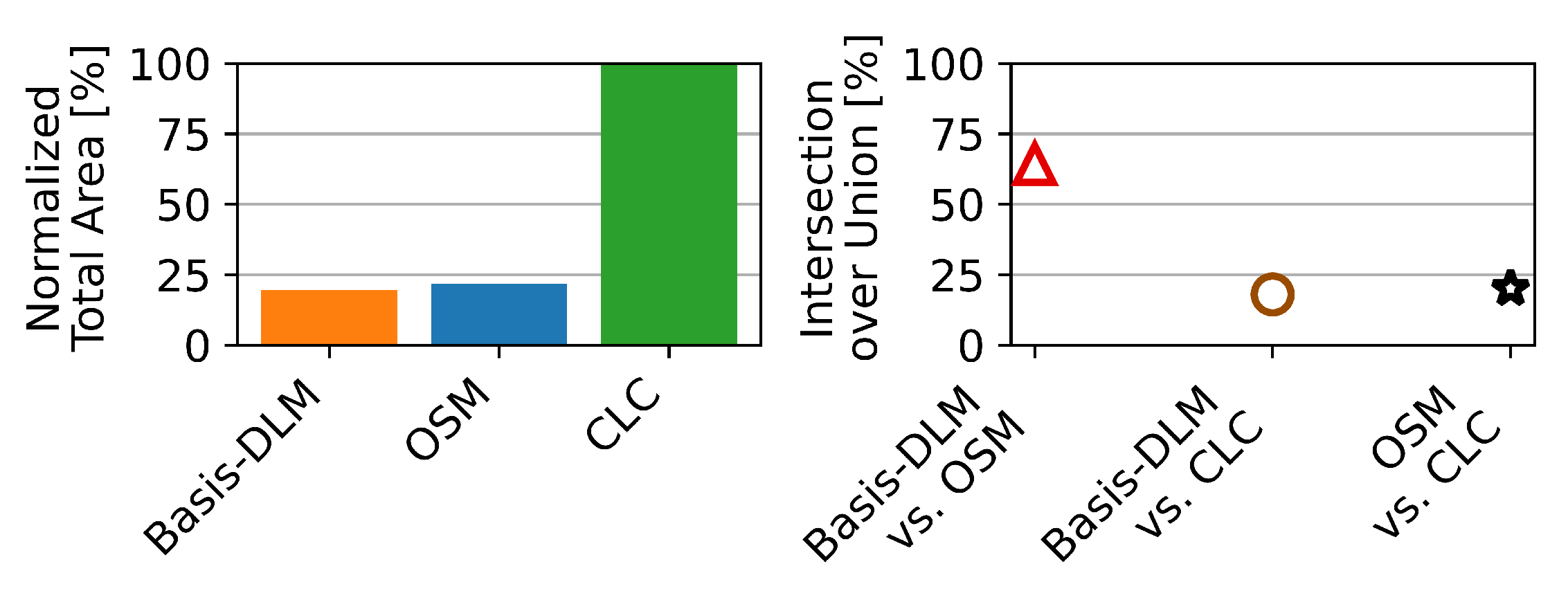
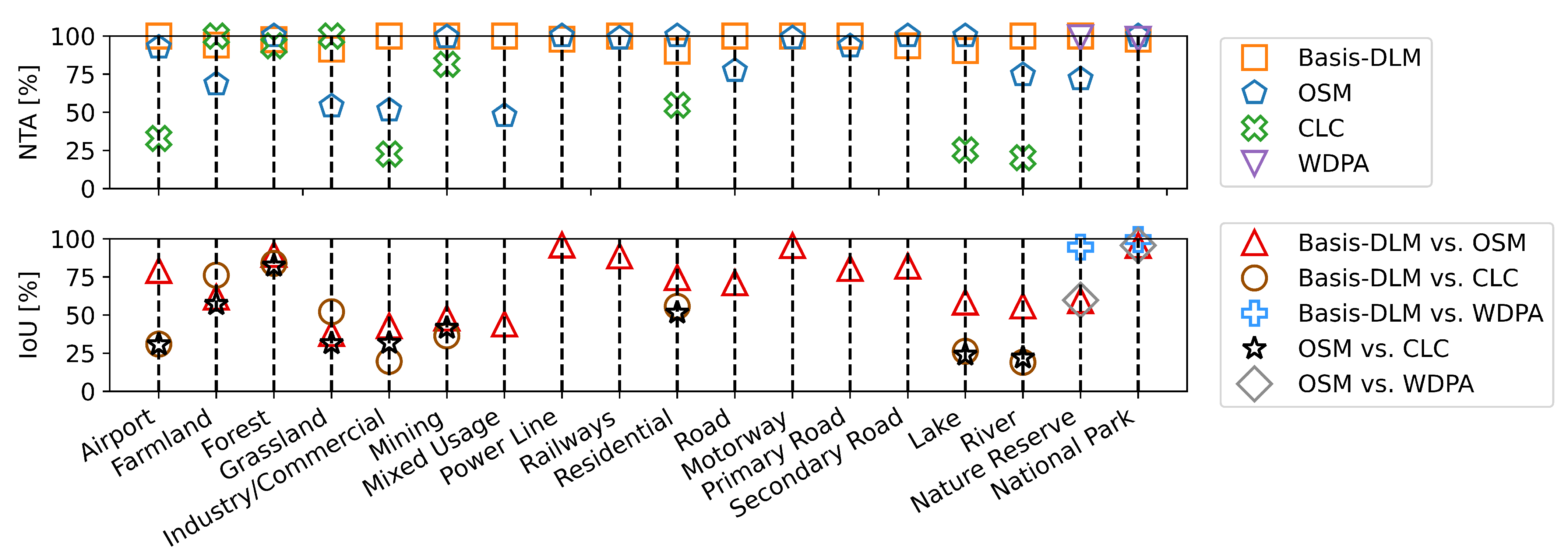
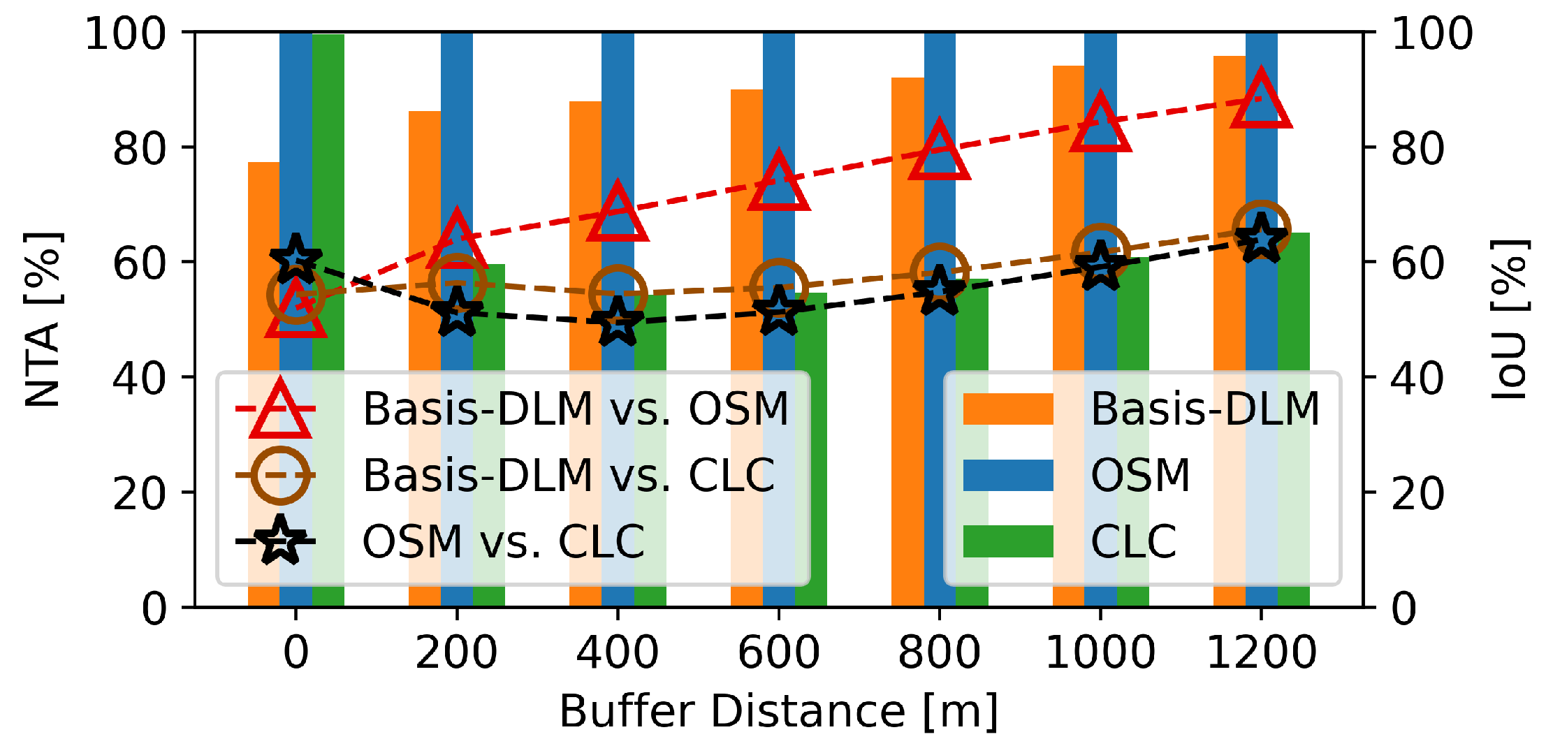
2.2. Evaluation of Land Use Datasets

To identify geographical features, land-eligibility analyses require geospatial datasets that describe land characteristics, e.g., land use, elevation, and water depths. The quality and resolution of the feature representation in the dataset, therefore, impacts the land-eligibility analysis. For instance, missing represented urban areas in a settlement dataset can underestimate areas that are excluded from the analysis of potential, and a coarse resolution can either under- or overestimate areas, depending on whether the pixel is mapped to a certain land-use category. For instance, a pixel representing a large area could have different land uses, but only be mapped to one. However, even though the datasets influence potential analyses, McKenna et al. [10] state that the impact of employing different data sources has not been evaluated to date.

In the present section, the first comparison and evaluation of the potntial of the following four land-use datasets is performed for the regional scope of Germany:

• Basis-DLM [12]: Official German dataset with a high positional accuracy (between ±3 and ±15 $\mathrm{m}$ depending on the feature).
• Corine Land Cover (CLC) [13]: Land cover raster dataset with 100 $\mathrm{m}$ × 100 $\mathrm{m}$ resolution. Available as a vector-representation, which is used in this section.
• Open Street Map (OSM) [14]: User-based land-cover vector dataset.
• World Database on Protected Areas (WDPA) [15]: Vector dataset with information on protected areas.

According to McKenna et al. [10], the CLC, OSM, and WDPA datasets are commonly used global and continental datasets for potential analyses.

Two parameters are used to compare the covered area using dataset $A\left(dataset\right)$ for multiple land-use categories, which are meaningful for land-eligibility analyses. For example, areas identified by the land-use category ‘Forest’ are compared for Basis-DLM, CLC, and OSM. The first parameter is the Normalized Total Area (NTA) (Equation (1)): This describes the area that was covered by a dataset compared to the maximum area covered by any other dataset capturing the feature:

$$NTA\left(datase{t}_i\right)=\frac{A\left(datase{t}_i\right)}{\underset{j}{max}(A\left(datase{t}_j\right)}$$

(1)

The second parameter is the Intersection over Union (IoU) of two datasets (Equation (2)): It describes the area identified by both datasets divided by the area identified when combining the two datasets. An Intersection over Union of $100\%$ describes the identified areas of two datasets as equal:

$$IoU\left(datase{t}_{(i,j)}\right)=\frac{A\left(datase{t}_i\right)\cap A\left(datase{t}_j\right)}{A\left(datase{t}_i\right)\cup A\left(datase{t}_j\right)}$$

(2)

The analysis was performed using additional standard setback distances, which are typically used for wind-potential analyses in the literature (see Supplementary Data). To this end, the features, which were identified by a dataset, were buffered using the chosen setback distances before calculating the Normalized Total Area and Intersection over Union. By using these setback distances, the wind potential analysis can reach a conclusion. Furthermore, a rasterized representation of the datasets, with their corresponding setback distance and a resolution of 10 $\mathrm{m}$ × 10 $\mathrm{m}$, is used.

Figure 1 shows the results for the Normalized Total Area and the Intersection over Union for the analyzed land-use categories.

The definition of the filter used to identify the respective features in each dataset can be found in the Supplementary Information.

It must be stated that the WDPA only provides information on protected areas, and its results are only comparable for these. Furthermore, the CLC does not include all presented categories, such as features with narrow widths such as roads or power lines.

In the exemplary wind-potential analysis, OSM and Basis-DLM identify the largest area and share the highest Intersection over Union for most categories. For the categories of farmland, forests, mining, and grassland, which are identified by their larger contiguous areas, the CLC classifies a similar area as Basis-DLM, which is identified by its large Normalized Total Area. Nevertheless, the Intersection over Unions are only high (above $70\%$) for the categories of farmland and forests, which means that the identified areas vary largely in the categories of mining and grassland. In the nature protection categories (‘Nature Reserve’, ‘National Park’), WDPA and Basis-DLM identify almost identical areas, which are recognizable through their Intersection over Unions of near $100\%$. The OSM-identified national parks are comparable to WDPA and Basis-DLM; however, the nature reserves show significant deviations from the Basis-DLM and WDPA.

McKenna et al. [10] and Masurowski et al. [16] state that the land-use category settlements (which are often synonymously used with residential land uses in land-eligibility analyses) highly influence the potential analysis in Germany, which is why this category is further analyzed.

For a typical setback distance of 1000 $\mathrm{m}$ in Figure 1, the OSM covers the largest area, followed by the Basis-DLM. Figure 2 shows how the Normalized Total Area and Intersection over Union of the residential category behaves when the setback distance is varied. Without any buffer, the OSM covers the largest area, closely followed by the CLC. With increasing setback distances, the Normalized Total Area of the CLC first drops rapidly, whereas the Normalized Total Areas of the Basis-DLM and OSM converge. This indicates that the Basis-DLM and OSM classify more, but smaller, settlements in comparison to the CLC. With increasing setback distances of above 600 $\mathrm{m}$, the Normalized Total Area of the CLC increases again, as the buffered areas around the smaller features identified by the Basis-DLM and OSM exhibit increasing overlap. The similarity between the Basis-DLM and OSM is also shown by their Intersection over Union, which increases over buffer distances of up to 88%. The described CLC behavior in the residential category, on the other hand, indicates that the representation of smaller detached settlements is missing, whereas larger settlements are covered to a coarser extent. This can be explained by the relatively coarse resolution of 100 $\mathrm{m}$ × 100 $\mathrm{m}$ found in the dataset and the minimum mapping unit (the smallest size at which a feature can be identified by a dataset) of 25 $\mathrm{h}\mathrm{a}$.

Using CLC to classify residential areas can lead to the underestimation of excluded areas and, therefore, an overestimation of potential areas, especially for typical setback distances for wind potential analyses between 600 and 1000 $\mathrm{m}$. Furthermore, CLC cannot represent categories with small features or short widths due to its minimal mapping unit. Therefore, the use of CLC for wind-potential analyses is not recommended.

The similarities between OSM and Basis-DLM can be seen for multiple categories, e.g., power lines and motorways, in which the Normalized Total Areas and Intersection over Unions are near $100\%$. For these categories, the use of both datasets is justified.

Figure 3 shows the results of a land-eligibility analysis with setback distances for the exemplary wind potential analysis (see the Supplementary Material) for Basis-DLM, OSM, and CLC. Analyses were performed for each dataset individually. To allow for comparison, the individual dataset was only used for features included in all three datasets; otherwise, a default dataset was applied for the exclusion (see Supplementary Data). Using CLC for land-eligibility analyses leads to significantly different results. The total potential area found when using the CLC is roughly $80\%$ higher compared to that found using OSM and Basis-DLM. However, the analyses conducted when using Basis-DLM and OSM, although resulting in similar total areas, contained discrepancies in locating the areas, as indicated by the Intersection over Union of $64\%$.

In summary, the presented analysis highlights the discrepancies in land-use declaration when using different datasets, meaning that the results of potential analyses using different datasets are hardly comparable. Furthermore, the analysis reveals the large sensitivity of land-eligibility results regarding the chosen datasets, and the importance of data with a high resolution and high positional accuracy for potential analyses.

For the scenarios outlined in this paper and the enclosed database, WDPA is used for the nature protection categories and Basis-DLM for most land-use categories in the land-eligibility analyses. Further datasets [17,18,19,20,21,22,23,24,25] were employed for other individual categories (e.g., water protection areas), but are not considered in this data analysis due to their lack of comparability to other datasets. Their documentation can be found in the Supplementary Data. Basis-DLM was selected due to its exhibited characteristics and is preferred over OSM due to its official character, high positional accuracy, detailed documentation, and the categories covered. Furthermore, for wind potential analysis, the residential areas are split into inner and outer areas (Inner areas (“Innenbereiche”) to refer to coherent built-up areas in accordance with §34 BauGB [26] and are modeled as the AX_Ortslagen features of Basis-DLM [12]. The residential buildings and other residential areas are treated as areas without a development plan (outer areas, “Außenbereiche”). Inner and outer areas can be protected differently, e.g., in the case of distance regulations for wind turbine constructions.), which is not possible with the sole use of OSM.

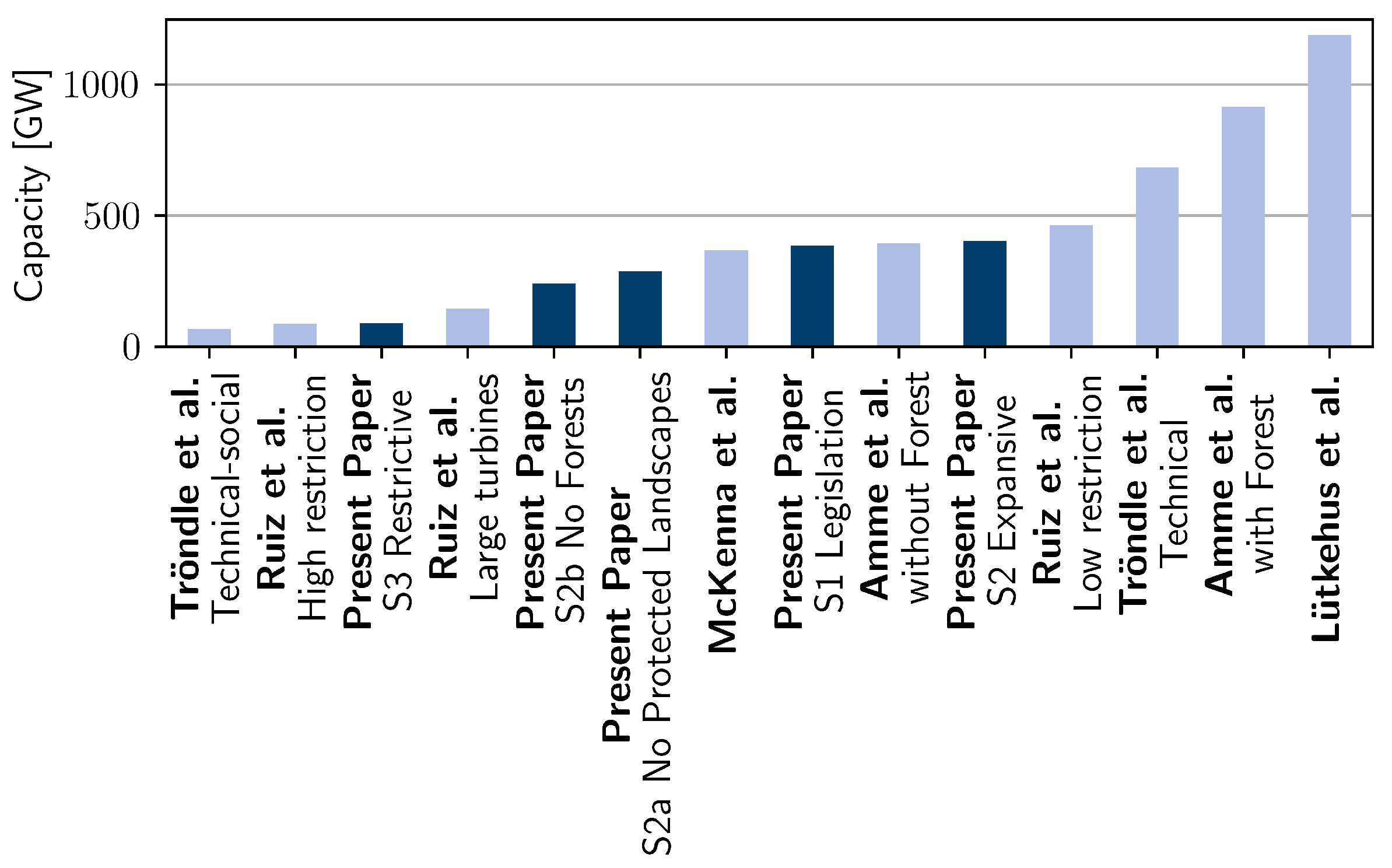
2.3. Onshore Wind Potential

2.3.1. Literature

Onshore wind analyses are generally performed with a greenfield approach (see, e.g., [4,27,28,29,30,31,32,33,34,35,36]). When applying a greenfield approach, all of the research subject’s area is initially, i.e., before applying exclusion criteria, assumed to be available. Only Masurowski et al. [16] proceed differently: First, initially available areas (pre-selected areas), such as grassland and arable land, are selected, and then further exclusion criteria are applied. For the considered studies, apart from the varying approach, the most influential differences correspond to the exclusion definitions, i.e., the used criteria and setback distances, the used data sources (cf. Section 2.2), and the estimation of the installable capacity on the determined eligible areas.

All of the cited studies pertain to residential areas. Nevertheless, the setback distances and the data sources significantly vary. Tröndle et al. [28] use the European Settlement Map [37] to identify built-up areas and exclude them without a buffer, whereas Peters et al. [30] and LANUV [31] differentiate the setback distance between inner (1000 $\mathrm{m}$) and outer areas (750, 720 $\mathrm{m}$) for their analysis based on Basis-DLM, and Amme et al. [32] use OSM [14] to identify residential areas and apply varying setback distances ( 400 to 1000 $\mathrm{m}$). Masurowski et al. [16] specify 1000 $\mathrm{m}$ for housing areas but vary the setback distance in their scenarios, without stating a data source. Others use CLC [13] to exclude settlements with 800 $\mathrm{m}$ [33,38] to 1000 $\mathrm{m}$ [39]. Ryberg et al. [33] additionally exclude urban areas from EuroStat Urban [40] with 1200 $\mathrm{m}$ setback. Lütkehus et al. [34] exclude residential areas with 600 $\mathrm{m}$ based on DLM250 [41]. Moreover, area-based residential, settlement, and urban exclusions of individual residential buildings are specified in two regional potential analyses [4,31,35].

Another frequently discussed topic is the construction of wind turbines in forests. The missing consensus in the legislation of the federal states can also be observed in the literature, i.e., Thuringia generally forbids the use of forests for wind turbines, whereas, in other federal states, the construction of these in forests is ongoing [42]. Ruiz et al. [27] exclude forests in the land eligibility analysis, whereas others [28,33] allow for construction in forests. Other studies treat forests in a differentiated manner. Coniferous forests in densely wooded municipalities are cited in the LANUV report [31]. Amme et al. [32] and Peters et al. [30] consider scenarios that include and exclude forests. Meanwhile, Ebner et al. [29] exclude forests in one scenario and allow for the construction in $10\%$ for another. Wiehe et al. [36] successively reduce the usable parts of forests in their more restrictive scenarios. Lütkehus et al. [34] exclude forests in federal states with less than $15\%$ forest shares. Furthermore, selective exclusions are performed based on the function of the forest.

Inconsistencies can also be seen for protected landscapes (Protected landscapes are areas protected by the German Federal Nature Conservation Act for its natural–ecological and cultural–social value [43]), which are a highly influential exclusion ($28\%$ of Germany’s area [15]). Several studies [30,32,34,36] regard protected landscapes differently in different scenarios, whereas others [33,35,38] generally rule out the construction of wind turbines in protected landscapes.

After determining the eligible areas, a few studies further reduce these, either by a certain share [28,29] or based on suitability factors [38,39] per CLC land-use category [13].

Based on the identified eligible areas, their capacity can be estimated. To this end, two different methods are utilized: The majority of analyzed studies [4,16,29,31,34,35,36] distribute turbines to eligible areas using a spacing distance specified by a multiple of the rotor diameter (D) in prevailing and transverse wind directions between the individual turbines. The turbine spacing ranges from 5 D to 9 D in the prevailing wind direction and 3 D to 4 D in the transverse direction. In contrast, others use fixed capacity densities, e.g., 5 $\mathrm{M}$$\mathrm{W}$/$\mathrm{k}$$\mathrm{m}$${}^2$ [27], 8 $\mathrm{M}$$\mathrm{W}$/$\mathrm{k}$$\mathrm{m}$${}^2$ [28], and 21 $\mathrm{M}$$\mathrm{W}$/$\mathrm{k}$$\mathrm{m}$${}^2$ [32]. Sensfuß et al. [39] and McKenna et al. [38] regionally vary the capacity density.

2.3.2. Methodology

The available area for onshore wind was determined using a greenfield land eligibility analysis (see Section 2.1). To this end, five different scenarios are defined:

• S1 Legislation: The exclusions are defined according to the laws of Germany’s federal states based on [44] and own corrections.
• S2 Expansive: Wind expansion favoring exclusions including forests and protected landscapes;
  S2a No Protected Landscapes: S2, excluding protected landscapes;
  S2b No Forests: S2, excluding forests.
• S3 Restrictive: Restrictive exclusions.

In scenario 1, federal state-specific exclusions are applied. The exclusions for each federal state are defined in accordance with Fachagentur Wind an Land [44], with expert-based corrections and additions for keys that cannot be directly retrieved from Fachagentur Wind an Land [44]. The definition of all exclusions can be found in the Supplementary Data.

In scenarios 2, 2a, 2b, and 3 nation-wide exclusions are applied. Scenario S2 Expansive refers to typical buffers at the lower end of the federal state’s legislation. The definitions can be found in the Supplementary Data. Additionally, the construction of wind turbines in forests is allowed. Scenarios 2a and 2b build upon scenario 2, but restrict construction in protected landscapes and forests. Scenario 3 refers to exclusions on the higher end of the setback distances in the legislation.

Table 1. Selected exclusion criteria for the scenarios of the wind onshore potential analysis.

Criterion	Data Source	S1 1	S2 2	S2a 2a	S2b 2b	S3 3
Inner areas	Basis-DLM [12]	individual *	1000 $\mathrm{m}$	1000 $\mathrm{m}$	1000 $\mathrm{m}$	1000 $\mathrm{m}$
Residential buildings, outer areas	Hausumringe [45]	individual *	3 H	3 H	3 H	1000 $\mathrm{m}$
Forests	Basis-DLM [12]	individual *	not excluded	not excluded	0 $\mathrm{m}$	0 $\mathrm{m}$
Protected Landscapes	WDPA [15]	individual *	not excluded	0 $\mathrm{m}$	not excluded	0 $\mathrm{m}$

¹ S1 Legislation; ² S2 Expansive; ^2a S2a No Protected Landscapes; ^2b S2b No Forests; ³ S3 Restrictive. * federal state-specific exclusions.

displays the most relevant of these.

Inner areas and outer areas are an influential exclusion. In the case of some federal state laws, residential areas in outer areas with a statute (Außenbereichssatzung) are protected in an identical manner to inner areas. For Scenario 1, we assume that all residential buildings are protected by such a statute.

Following the land-eligibility analysis, areas smaller than $0.01$ $\mathrm{k}$$\mathrm{m}$${}^2$ are excluded.

To estimate the capacity potential, we classify turbines with GLAES [46] in the eligible areas. To this end, a spacing distance of 8 D × 4 D is used. A typical low wind (wind class IEC IIIB) $4.7$ $\mathrm{M}$$\mathrm{W}$ turbine with a 155 $\mathrm{m}$ rotor diameter and 120 $\mathrm{m}$ hub height is used as the reference turbine model.

2.3.3. Results & Discussion

Table 2. Results for the scenarios of the onshore wind potential analysis at the national level.

	S1 1	S2 2	S2a 2a	S2b 2b	S3 3
Area [$\mathrm{k}{\mathrm{m}}^2$]	24,663	25,938	17,613	10,056	3923
Area Share [%]	6.89	7.25	4.92	2.81	1.10
Capacity [$\mathrm{G}\mathrm{W}$]	385	403	287	241	90
Density on eligible areas [$\frac{\mathrm{M}\mathrm{W}}{\mathrm{k}\mathrm{m}{}^2}$]	15.6	15.5	16.3	23.9	22.8

¹ S1 Legislation; ² S2 Expansive; ^2a S2a No Protected Landscapes; ^2b S2b No Forests; ³ S3 Restrictive.

shows the main results of the scenarios at the national level. In Scenario S2 Expansive, $7.25\%$ of Germany’s area is usable for wind turbines, which leads to a capacity potential of 403 $\mathrm{G}$$\mathrm{W}$. Figure 4 visualizes its capacity density per municipality in relation to the area of the municipality. The potentials are evenly distributed over Germany; only North Rhine-Westphalia has larger areas without any potentials due to its high population density.

Scenario S3 Restrictive leads to only 90 $\mathrm{G}$$\mathrm{W}$ on $1.1\%$ of Germany’s land. The capacity densities in the scenarios S1 Legislation, S2 Expansive, and S2a No Protected Landscapes are smaller than they are in scenarios S2b No Forests S2b and S3 Restrictive, due to the larger contiguous areas in the scenarios not excluding forests, i.e., S1, S2, and S2a. In the larger areas, the distance between the turbines is more apparent as smaller areas naturally have spaces between them.

Two potential analyses at the federal state level [31,35] are used to validate the workflow. To this end, the same datasets and the same exclusion definitions are used. The area potential adds up to $103.3\%$ and $96\%$ in relation to the study in Baden-Württemberg [35] and Northrhine-Westphalia [31], respectively. When compared with the Landesanstalt für Umwelt Baden-Württemberg [35], an Intersection over Union of $79.3\%$ is achieved. The differences can be explained by the versions of Basis-DLM [12] and unclear definitions of single exclusions.

Figure 5 shows the range of 68 $\mathrm{G}$$\mathrm{W}$ to 1188 $\mathrm{G}$$\mathrm{W}$ of onshore wind potential values in the literature. The results are influenced by the use of different datasets (see Section 2.2), exclusion definitions, area correction factors, and capacity estimation methods.

Ruiz et al. [27], Tröndle et al. [28] and McKenna et al. [38] utilize, amongst others, CLC for land-use classification, which we show to be problematic for potential analyses (Section 2.2). Furthermore, Tröndle et al. [28], in technical–social scenarios and McKenna et al. [38] correct the estimated areas using correction and suitability factors for land-use categories, respectively. These approaches are not comparable to our results, which clearly indicate locations as being either eligible or ineligible. Amme et al. [32] outlined a scenario excluding residential areas with a 1000 $\mathrm{m}$ setback distance as well as protected landscapes, but allowing forests, which is comparable to our scenario: S2a No Protected Landscapes. By comparing the results, Amme et al. [32] exceed the presented eligible area and capacity by factors of 2.47 and 3.18, respectively. Lütkehus et al. [34] use comparably low setback distances, e.g., 600 $\mathrm{m}$ to inner areas, and do not exclude residential buildings, leading to their having the highest capacity potential of the considered studies. This emphasizes the impact of the chosen exclusion criteria and setback distances. Furthermore, they use the land-use dataset DLM250 [41] with a positional accuracy of ±100 $\mathrm{m}$, which can lead to inaccuracies when identifying features.

There is no consensus on exclusions and setback distances in wind potential analyses. One exclusion criterion used by all of the cited studies is residential areas. Nevertheless, individual residential buildings are often neglected due to data availability issues. In our scenarios, neglecting residential buildings leads to significantly higher capacity potentials ($27\%$, $9\%$, $10\%$, $12\%$, and $34\%$). For regional or federal state analyses, this error is even more apparent: For example, in Schleswig Holstein, the potential is overestimated by $56\%$, $25\%$, $25\%$, $27\%$, and $100\%$. To the authors’ knowledge, no national potential analysis with published results has excluded buildings. In future work, a focus on sensitivity regarding exclusion definitions could help to make such effects more transparent. Additionally, the sensitivities of certain exclusion criteria, e.g., forests or buildings, could help legislators to quantify the impact of their decisions. Our restrictive scenario results in a potential of 90 $\mathrm{G}$$\mathrm{W}$, which is not sufficient to reach Germany’s climate goals according to different studies [3,4,5,9] and underlies the importance of liberal legislation regarding wind expansion.

Furthermore, the chosen turbine has a large impact on the capacity density, as well as on the land-eligibility analyses via height- or diameter-dependent exclusions. We selected a typical wind turbine for low wind speeds (cf. Section 2.3.2). When using a turbine for medium wind speeds (IEC II, 5 $\mathrm{M}$$\mathrm{W}$ capacity, 145 $\mathrm{m}$ diameter) with the same hub height, the capacity potential increases by $16.2\%$, to $19.5\%$, in our scenarios. In future, site-specific turbine selection could help improve the results in this regard and sensitivity analyses could be performed for the turbine design and the spacing between turbines. Nevertheless, with respect to the chosen low wind-speed turbine, the results are still robust. Only $2\%$ and $29\%$ of the determined locations, respectively, reach an average wind speed IEC II wind class in 100 $\mathrm{m}$ and 150 $\mathrm{m}$ height [47].

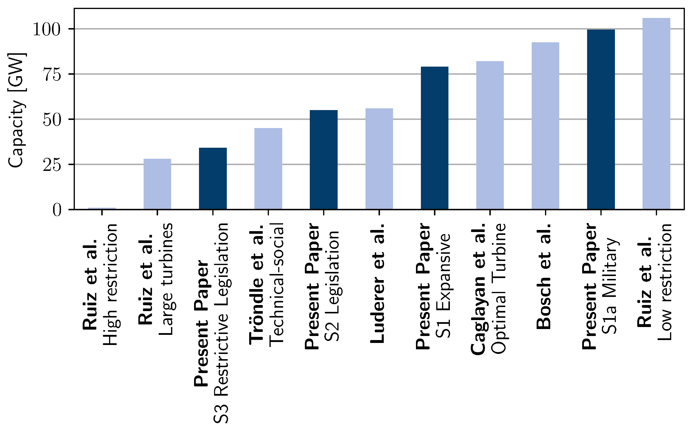
2.4. Offshore Wind Potential

2.4.1. Literature

The following section provides an overview of the offshore wind potential analyses found in the literature. The regional coverage of the analyzed studies varies between global [48,49], European [27,28,29,50] and national [4] studies. As a first step in the potential analyses, eligible areas are determined. Most studies [27,28,29,49,50,51] use greenfield approaches, initially considering the sea to be eligible and applying exclusion criteria. Sensfu et al. [52], however, followed a mixed approach of greenfield analysis and pre-selected areas in their global analysis. For Germany, 80% of the declared offshore wind areas in 4C Offshore [53] were used as pre-selected areas. Luderer et al. [4] considered the wind farm areas of the draft of the Area Development Plan 2020 [54] and areas of existing plants [55] as pre-selected.

The studies that follow the greenfield approach often use similar exclusion criteria, but differ in terms of dataset, methods, and buffer distances. Common exclusion criteria include, amongst others, distance to shore, sea depth, protected areas, shipping routes, and infrastructures. The minimal distance to shore varies between 10 $\mathrm{k}$$\mathrm{m}$ [49] and $22.2$ $\mathrm{k}$$\mathrm{m}$ [27]. The exclusion of areas with large sea depths differs between depths lower than 50 $\mathrm{m}$ [27,28,50], 100 $\mathrm{m}$ [27], 1000 $\mathrm{m}$ [29,49,51], or unlimited [50]. Shipping routes are excluded by Ruiz et al. [27] and Caglayan et al. [51] based on the Halpern et al. [56] dataset, which addressed the likelihood of ships. Furthermore, Caglayan et al. [51] manually exclude known routes with a buffer of 4 $\mathrm{k}$$\mathrm{m}$. Ebner et al. [29] exclude shipping routes, without noting a methodology or data source. Additionally, certain studies [27,49,51] exclude infrastructure, e.g., cables and pipelines with buffers from 500 $\mathrm{m}$ [51] to $7.4$ $\mathrm{k}$$\mathrm{m}$ [27]. After applying the exclusion criteria, Zappa and van den Broek [50] and Tröndle et al. [28], in their technical–social scenario, reduce the resulting eligible areas to 20% and 10%, respectively. Zappa and van den Broek [50] explain the reduction by a set factor due to missing exclusion categories.

The potential offshore wind capacity can be estimated for the eligible areas. Most presented studies employ an aggregated method with capacity density factors ranging from $3.14$ $\mathrm{M}$$\mathrm{W}$/$\mathrm{k}$$\mathrm{m}$${}^2$ [49] to 15 $\mathrm{M}$$\mathrm{W}$/$\mathrm{k}$$\mathrm{m}$${}^2$ [28]. Ebner et al. [29] reduce 14 $\mathrm{M}$$\mathrm{W}$/$\mathrm{k}$$\mathrm{m}$${}^2$ to 5 $\mathrm{M}$$\mathrm{W}$/$\mathrm{k}$$\mathrm{m}$${}^2$ due to a deviation in the results by a factor of 3 from the German Bundesfachplan 2017 [57,58]. Other studies [4,52] use a variable capacity density per eligible area. Only Caglayan et al. [51] employed a placing algorithm for wind turbines with a turbine spacing of 10 D × 4 D.

2.4.2. Methodology

The offshore wind potential analysis was performed for federal states in the coastal sea and Exclusive Economic Zones (EEZ) in the Northern and Baltic sea areas. Four different scenarios were considered:

• S1 Expansive: Greenfield analyses with offshore wind expansion favoring exclusions
  S1a Military: S1, including the usage of military areas.
• S2 Legislation: Current priority and reservation areas for offshore wind in legislation.
• S3 Restrictive Legislation: Current priority areas for offshore wind in legislation.

The Low-Exclusion Scenarios S1 and S1a are greenfield approaches that use exclusion criteria with comparably low exclusion definitions. The following describes the main exclusions; full information about these can be found in the Supplementary Data. Areas within 15 $\mathrm{k}$$\mathrm{m}$ of the shore and 500 $\mathrm{m}$ of the sea border to neighboring countries are considered ineligible. To address shipping land use, declared priority shipping areas of the current legislation of the EEZ [59] and federal states [60,61,62] were excluded with a buffer of 500 $\mathrm{m}$. Furthermore, infrastructure facilities, e.g., cables and platforms, were excluded by CONTIS [63] with 500 $\mathrm{m}$. The scenarios S1 Expansive and S1a Military differ in the consideration of designated military areas, which cover a significant share of the German coastlines. As military areas overlap with designated wind areas in the current legislation, the exclusion of all military areas is not realistic. However, the exclusion of individual sub-areas is not possible due to a lack of indications regarding the suitability of mixed use. Only Scenario S1 Expansive further excluded declared military areas according to CONTIS [64] and ROP [59].

The scenario S2 Legislation considers all designated areas for offshore wind as pre-selected areas, whereas scenario S3 Restrictive Legislation only considers the priority and conditional priority areas. The definition of these areas is based on the current legislation of the EEZ [59], Lower Saxony [60], and Mecklenburg-Western Pomerania [61]. Schleswig Holstein and Hamburg do not designate areas for offshore wind [65,66]. The legislation scenarios S2 and S3 further apply the infrastructure exclusions described in Low-Exclusion Scenarios S1 and S1a.

After employing the exclusion scenarios, eligible areas with a resulting size smaller than $0.1$ $\mathrm{k}$$\mathrm{m}$${}^2$ were excluded.

The potential capacity of the scenarios is estimated with a similar approach as that used for onshore wind (Section 2.3.2) by using the turbine placement of GLAES [46] and a turbine spacing of 8 D × 4 D, respectively. A reference turbine with a capacity of 8 $\mathrm{M}$$\mathrm{W}$ and a rotor diameter of 167 $\mathrm{m}$ is used.

2.4.3. Results & Discussion

The results of the offshore potential analysis at the national level are presented in

Table 3. Results for the offshore wind potential analysis at the national level.

	S1 1	S1a 1a	S2 2	S3 3
Area [$\mathrm{k}{\mathrm{m}}^2$]	7353	9275	5174	3182
Area Share [%]	13.07	16.48	9.19	5.65
Capacity [$\mathrm{G}\mathrm{W}$]	79.1	99.6	55.8	34.1
Density on eligible areas [$\frac{\mathrm{M}\mathrm{W}}{\mathrm{k}\mathrm{m}{}^2}$]	10.75	10.74	10.79	10.71

¹ S1 Expansive; ^1a S1a Military; ² S2 Legislation; and ³ S3 Restrictive Legislation.

and show a range between $34.1$ $\mathrm{G}$$\mathrm{W}$ (S3 Restrictive Legislation) and $99.6$ $\mathrm{G}$$\mathrm{W}$ (S1a Military).

It is possible to increase the potential of the current legislation, i.e., S2 and S3, by limiting other declared land uses, such as shipping or military areas. However, the possible increase in capacity potential differs between the Northern and Baltic seas. From scenario S2 legislation to S1 expansive, the potential is increased by $21.6$ $\mathrm{G}$$\mathrm{W}$ in the North Sea and $1.6$ $\mathrm{G}$$\mathrm{W}$ in the Baltic. When comparing S2 legislation to S1a military, the increase in capacity is higher, with 39 $\mathrm{G}$$\mathrm{W}$ and 5 $\mathrm{G}$$\mathrm{W}$, respectively. Thus, by redefining and limiting other declared land uses in legislation as military or shipping areas, further areas could be designated for offshore wind, especially in the North Sea. Future work could critically revise these areas or consider their combined usage with offshore wind projects.

Furthermore, the reference turbine impacts the capacity potential. To quantify the impact, Scenario S1 was recalculated with a 11 $\mathrm{M}$$\mathrm{W}$ turbine ( 200 $\mathrm{m}$ rotor diameter). The capacity potential decreased by 1.4%; however, 28.27% fewer turbines are required. In the future, site-specific turbine designs and a sensitivity analysis for turbine selection could be applied.

The results of the presented scenarios are compared to the literature in Figure 6. The scenarios S1 expansive and S1a military follow the greenfield approach, which is comparable to all considered studies, except for that of Luderer et al. [4]. Luderer et al. [4], who use the same designated wind farm area of BSH leading to 56 $\mathrm{G}$$\mathrm{W}$, had comparable results to $55.8$ $\mathrm{G}$$\mathrm{W}$ in the present scenario, S2 Legislation.

For the greenfield analyses, none of the presented studies use the official German data, e.g., data for shipping or military areas. Two Ruiz et al. [27] scenarios and the technical–social scenario of Tröndle et al. [28] even undercut the potential capacity results of our scenarios: S2 legislation and S3 restrictive legislation. Ruiz et al. [27], in their low-exclusion scenario, and Bosch et al. [49] have capacity potentials that are comparable to S1a. However, as the capacity densities of our study are around two and three times higher than their studies, respectively, this indicates that there are significantly fewer eligible areas in our scenarios. The comparisons show the impact of data sources, exclusions, and capacity densities on land-eligibility analyses and capacity estimations.

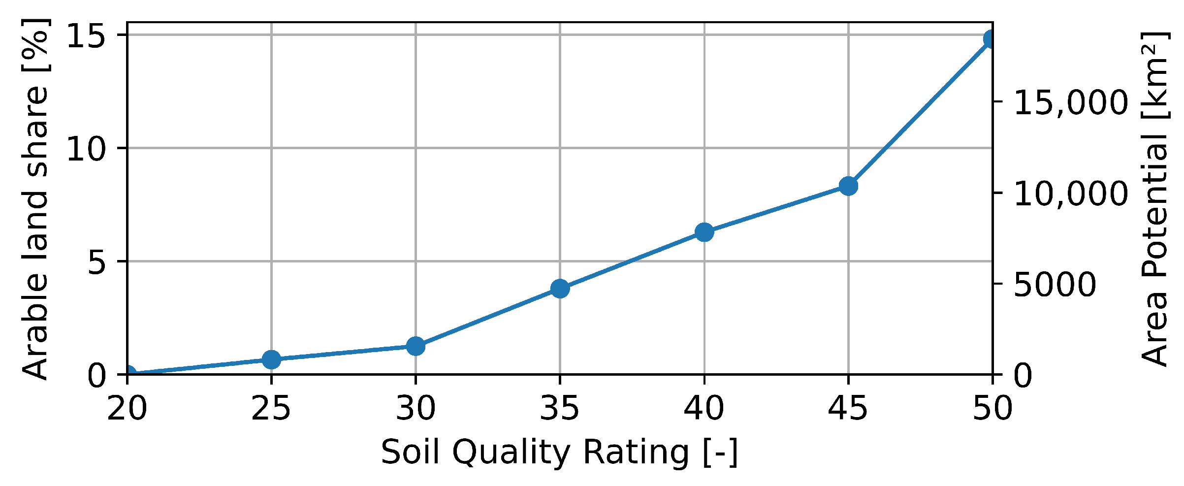
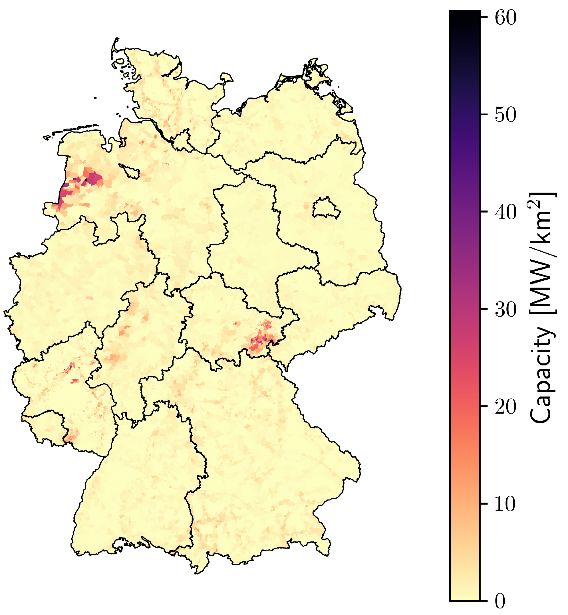
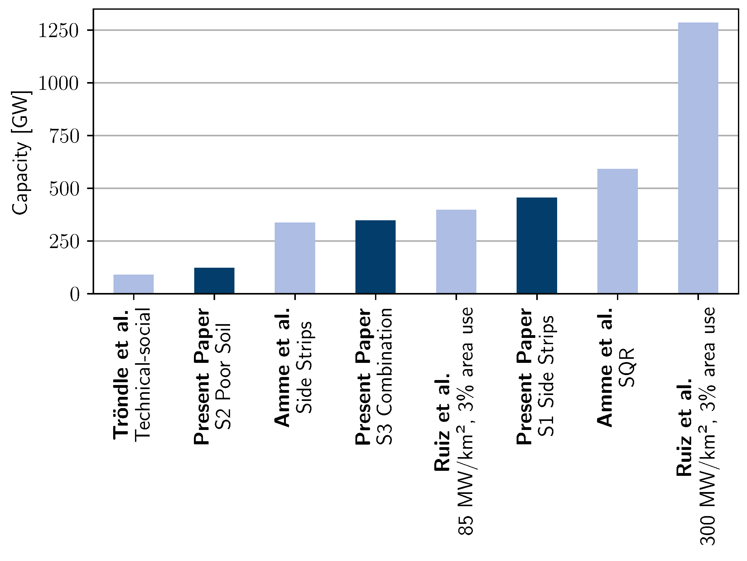
2.5. Open-Field Photovoltaic Potential

2.5.1. Literature

Although wind potential analyses mostly use greenfield approaches in landeligibility analysis (see Section 2.3), open-field PV potential analyses often first consider pre-selected areas as being eligible and then apply further exclusion criteria [4,27,28,29,32,67,68,69]. Only a few potential analyses choose a greenfield exclusion approach [30,70].

However, as the pre-selected areas highly differ accross studies, several examples are presented: Ruiz et al. [27] and Tröndle et al. [28] estimate the potential for Europe and consider land-use categories as pre-selected areas, which leads to a high area potential for open-field PV. Ruiz et al. [27] define, amongst others, bare land, some cropland, and some eligible classes of vegetation, and use a combination of Global Land Cover [71] and Corine Land Cover [13] to identify these. This leads to an initial eligible area of $44\%$ of Germany, from which a share of $3\%$ is considered eligible in another scenario. Tröndle et al. [28] consider $10\%$ of bare and unused land defined by GlobeCover2009 [72] as pre-selected areas in a technical–social potential analysis. Lux et al. [67] define certain shares of categories of CLC [13] eligible, e.g., $16\%$ of bare land and $2\%$ of bushland. Meanwhile, Ebner et al. [29] consider agriculture and grazing land identified by CLC [13] in less-favored regions [73] as eligible for technical potential. However, this is further reduced to $7\%$ of the pre-selected area, which is $50\%$ of the area share that is currently used for energy crops. Several studies with the scope of Germany follow the legislation of the Renewable Energy Act (EEG) [74]. Amongst other areas, the EEG considers less-favored areas and side strips of motorways and railways to be eligible. The potential areas along side strips are either defined by a 110 $\mathrm{m}$ width, in accordance with EEG 2017 [75], or a 200 $\mathrm{m}$ width, in accordance with EEG 2021 [74], minus a 15 $\mathrm{m}$ animal migration buffer. Luderer et al. [4] also use side strips, but consider 185 $\mathrm{m}$ around the line objects of OSM, therefore neglecting the width of the road and the animal migration corridor. Furthermore, they consider agricultural land with poor soil quality, which is defined with the dataset Soil Quality Rating (SQR) [76] and a threshold of 40. Amme et al. [32] similarly consider less-favored areas, but also consider side strips with a width of 500 $\mathrm{m}$, which corresponds to 2.7 times the current legislation. Agricultural land with a soil quality rating higher than 40 are excluded within the side strips. Other EEG-favored areas are also neglected due the availability of data and small resulting areas. Several studies perform potential analyses at the federal state level in Germany, e.g., Seidenstücker [69] for North Rhine-Westphalia and Landesanstalt für Umwelt Baden-Württemberg [68] for Baden-Württemberg. Both studies use input datasets with local coverage and high resolutions, e.g., Basis-DLM [12], and estimate the potential for the side strips of 110 $\mathrm{m}$ of railway and roads in accordance with the legislation of EEG 2017 [75].

After defining the pre-selected areas, further exclusion criteria can be applied, resulting in eligible areas of various shapes and sizes. As it is not economically feasible to install open-field PV sites in small eligible areas, several studies exclude areas smaller than a certain threshold. The threshold can vary in the range from 500 $\mathrm{m}$${}^2$ [69] to 100,000 $\mathrm{m}$${}^2$ [32].

As the second step of the potential analysis, the installable open-field PV capacity on eligible areas is estimated. Open-field PV potential analysis uses an empirical factor of the capacity density in $\mathrm{M}$$\mathrm{W}$/km${}^2$. However, the literature reports a high range, from 40 $\mathrm{M}$$\mathrm{W}$/km${}^2$ in [29] to 300 $\mathrm{M}$$\mathrm{W}$/km${}^2$ [27]. Ebner et al. [29] explain the factor of 40 $\mathrm{M}$$\mathrm{W}$/km${}^2$ based on an aerial photo evaluation of existing open-field PV systems. Tröndle et al. [28] explain their value of 80 $\mathrm{M}$$\mathrm{W}$/km${}^2$ with a module efficiency of $16\%$ and $50\%$ area reductions by row placements to prevent shadowing. Seidenstücker [69] assume a module efficiency of $17\%$ and an area reduction of $50\%$ for slopes less than 20°, leading to 85 $\mathrm{M}$$\mathrm{W}$/km${}^2$. Wirth [77] reports a value of 100 $\mathrm{M}$$\mathrm{W}$/km${}^2$ based on row spacing and a module efficiency of $20\%$.

2.5.2. Methodology

In the first step of the potential analysis for open-field PV pre-selected areas are considered eligible, followed by further exclusions. To this end, three scenarios are regarded:

• S1 Side Strips: Side strips of motorways and railways in accordance with the subsidy areas of the EEG 2021 [74].
• S2 Poor Soil: Arable land with barren soil based on the Soil Quality Rating (SQR) of [76].
• S3 Combination: Side strips, for which arable land is restricted to SQR $<40$, and S2.

Scenario S1 Side Strips estimate the potential of the side strips of motorways and railways. Their routes and widths were identified by Basis-DLM [12]. Then, side strips of 200 $\mathrm{m}$ were used, from which 15 $\mathrm{m}$ on the inside is subtracted for animal migration. The remaining area represents the pre-selected area.

Scenario S2 Poor Soil pre-selects arable land with bad soil quality based on the SQR dataset [76]. The SQR threshold was chosen to be 30 based on pre-analysis. Figure 7 shows the area potential and share of arable land for SQR limits between 20 and 50. As is shown in Section 2.5.1, other potential studies use a threshold of 40, which results in $6.28\%$ of arable land. We assumed this to be too ambitious due to land-use conflicts with the cultivation of arable land, and therefore chose the threshold of 30. All areas up to a selected SQR value were intersected with the arable land in Germany from Basis-DLM [12] due to the 100 $\mathrm{m}$ × 100 $\mathrm{m}$ resolution in the BGR rating [76].

Scenario S3 Combination is a combination of a pre-selection using side strips and arable land with barren soil. As side strips are considered less valuable than other areas, arable land with SQR values of less than 40 was excluded. On all other arable land, only SQR values of less than 30 were used in pre-selection. It should be noted that land uses other than agricultural inside the side strips were not restricted by the SQR rating.

After identifying pre-selected eligible areas for each scenario, unsuitable areas within these were deducted according to the further exclusion criteria.

Table 4. Selected exclusion criteria for the scenarios of the open-field PV potential analysis.

Criterion	Data Source	S1 Side Strips	S2 Poor Soil	S3 Combination
Forests	Basis-DLM [12]	10 $\mathrm{m}$	10 $\mathrm{m}$	10 $\mathrm{m}$
All Buildings	Hausumringe [45]	10 $\mathrm{m}$	10 $\mathrm{m}$	10 $\mathrm{m}$
Arable land	Basis-DLM [12], SQR [76]	not excluded	SQR $\ge 30$	SQR $\ge 30$, Sidestripes: SQR $\ge 40$
Motorways, Railways	Basis-DLM [12]	15$\mathrm{m}$	200 $\mathrm{m}$	15 $\mathrm{m}$

displays the most relevant exclusions. The definition of all exclusions can be found in the Supplementary Material. After the land-eligibility analysis, eligible areas smaller than a threshold of 5000 $\mathrm{m}$${}^2$ were excluded for economic reasons, which lies within the range of the presented literature (see Section 2.5.1). However, this area threshold leads to a deviation of eligible areas at different regional levels. Areas may become ineligible if they are split by a border to a size lower than the threshold size, whereas those at a higher regional level are still eligible. For the three scenarios, this leads to a capacity deviation from $1.3\%$ to $1.5\%$ between the federal state and the municipality level.

As a next step in the potential analysis, the installable capacity on the eligible land was estimated. Therefore, the eligible areas and their size $A_{OFPV}$ were extracted. This area can be converted by applying a capacity density, as described in Equation (3):

$$P_{OFPV}={\displaystyle \frac{f_{GC}·f_c}{a_{coverage}}}·A_{OFPV}=79.2\mathrm{M}\mathrm{W}/\mathrm{k}{\mathrm{m}}^2·A_{OFPV}$$

(3)

where $f_{GC}=0.5$ and $f_c=0.72$ [78] were used to take the ground coverage of the modules and construction-related obstructions into account. $a_{coverage}=4.55 {\mathrm{m}}^2/\mathrm{k}\mathrm{W}$ is the direct module coverage, which corresponds to an efficiency of $0.22$, in line with current high-end modules [79,80].

2.5.3. Results & Discussion

The results at the national level for the potential area and the capacity of the scenarios are shown in

Table 5. Results for the scenarios of the open-field PV potential analysis at the national level.

	S1 1	S2 2	S3 3
Area [$\mathrm{k}{\mathrm{m}}^2$]	5723	1560	4373
Area Share [%]	1.60	0.44	1.22
Capacity [$\mathrm{G}{\mathrm{W}}_{\mathrm{p}}$]	456.1	123.6	347.7
No. of Municipalities in Germany	11,003	11,003	11,003
⋯ with pre-selected areas	5667	1892	6446
⋯ with potential	5253	1711	5939

¹ S1 Side Strips; ² S2 Poor Soil; and ³ S3 Combination.

. The capacity potential varies between $123.6$ $\mathrm{G}$$\mathrm{W}$p in S2 Poor Soil and $456.1$ $\mathrm{G}$$\mathrm{W}$p in S1 Side Strips. Figure 8 visualizes the capacity density for the scenario S3 Combination per municipality in relation to the area of the municipality. Noticeably, the potential concentrates in regions in Thuringia and lower saxony.

To validate the presented workflow, two potential analyses at the federal state level [68,69] were used, due to their high spatial resolutions and use of local data. Similarly to Side Strips S1, the studies consider pre-selected areas at the sides of roads and railways. Using similar exclusion criteria and datasets as the corresponding studies, an Intersection over Union of $81.38\%$ was achieved for Landesanstalt für Umwelt Baden-Württemberg [68] and $87.88\%$ for Seidenstücker [69]. The area potential of the presented workflow in relation to that reported by [68] and [69] is $88\%$ and $103\%$, respectively.

Differences between the results of the studies and this paper arise due to the different land cover datasets and unclear definitions of single exclusions.

As shown in Figure 9, the literature provides a wide range of 90 $\mathrm{G}$$\mathrm{W}$p [28] to 1285 $\mathrm{G}$$\mathrm{W}$p [27] as capacity potentials for open-field PV because the pre-selected areas, used datasets, area reduction factors, and applied exclusion criteria widely differ between the studies (cf. Section 2.5.1). Furthermore, the capacity density factors varied greatly between the studies, which leads to further deviations. Ruiz et al. [27] and Tröndle et al. [28] used set shares, $3\%$ and $10\%$, respectively, of large land-use categories for the land-eligibility analyses, and are not comparable with our scenarios.

Methodology-wise, our scenarios are only comparable to Amme et al. [32]. For the presented SQR scenario, the higher potential capacity of Amme et al. [32] can be explained by its higher SQR threshold. For the side strips’ scenario, Amme et al. [32] use side strips that are 2.7 times the width of the current legislation. Nevertheless, by additionally excluding areas with an SQR higher than 40, the resulting capacity is lower than it is in our scenario S1 Side Strips.

The presented workflow could be further extended by considering other subsidy-areas of the Renewable Energy Act [74], such as dumps and landfills, as pre-selected areas. Furthermore, categories beyond the scope of the current legislation could be chosen as pre-selected areas. However, there is no consensus in the literature regarding eligible land-use categories and considering entire categories as eligible tends to lead to high potentials, as in Ruiz et al. [27]. Such high area shares are critical due to the land-use conflicts they can induce: whereas wind turbines only occupy a share of their designated areas, open-field PV plants cover most of their appointed ones, which can lead to conflicts with, for example, agricultural land use. Furthermore, legislation has a significant impact on the distribution of potentials. In open-field PV scenarios, many municipalities have no potential (cf. Table 5), due to the limitation to municipalities with subsidy-eligible areas. This can lead to unequally distributed economic benefits among municipalities, as well as higher resistance in society due to, for instance, visual impacts. As the results are also highly sensitive to the chosen capacity density factor, one avenue of further work could be to incorporate future system designs. Additionally, the effect of placing the modules flat or in an east–west orientation without any row-spacing could be analyzed.

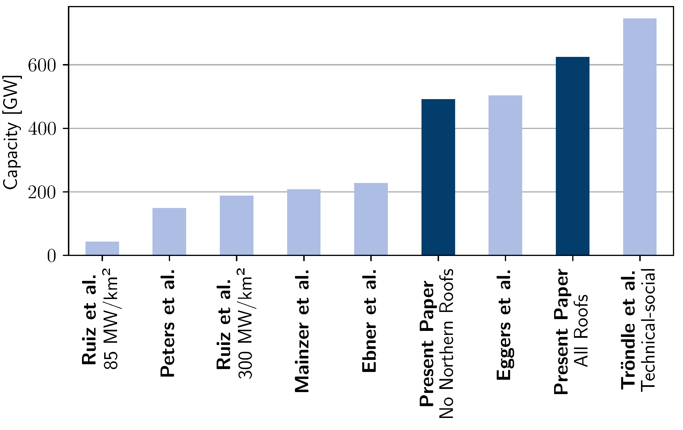
3. Rooftop Photovoltaic Potential

In the following chapter, the assessment of rooftop PV potential for Germany is discussed. First, an overview of the literature is presented (Section 3.1). Then, the methodology for extracting potential from 3D building data is described (Section 3.2). The results are then presented and discussed (Section 3.3).

3.1. Literature

Rooftop PV potential analyses can be classified by their geographical extent and the resolution of their results [81,82].

The resolution of different approaches can be split into high, medium, and low levels. High-level approaches, which can assess the potential for individual buildings include, for example, image recognition techniques [83,84,85,86] or workflows using 3D building models [87,88,89,90,91]. For instance, Grothues and Seidenstücker [87] determine all roof geometries in North Rhine-Westphalia on the basis of laser scan data at $0.5$ $\mathrm{m}$ × $0.5$ $\mathrm{m}$ resolutions. Low- and medium-level approaches mostly base their analysis mostly on statistical data and are, therefore, limited to the assessment of potentials for the regional scope of the data, e.g., to regions, countries, or raster resolution [27,28,29,30,82,92,93,94,95]. Tröndle et al. [28], for instance, use population data from the European Settlement Map [37] to estimate roof areas and calibrate them with data from sonnendach.ch [96]. Meanwhile, Ruiz et al. [27] use CLC [13] data to identify residential and industrial areas in which they estimate roof areas based on fixed factors.

The geographical extent of these analyses varies from single buildings to continent-wide. Statistical approaches are mainly used to perform large-scale analyses, such as at national [29,30,82,95] or continental scales [27,28,94]. However, more recent studies were able to apply high-level methodologies to the national scale. Walch et al. [89] use LoD2 3D data to extract rooftop PV potential in Switzerland. To this end, they calculated the area and orientations of 9.6 million rooftops directly from the data. Luderer et al. [4] estimated the rooftop PV potential in Germany at the municipality level by correlating it with building footprints in a region. Similarly, Wiehe et al. [36] used building footprints in Germany and building use to estimate generation potential. Eggers et al. [97] use LoD1 building models (without information on rooftop geometry) to estimate German rooftop PV potential.

Approaches, that use data without information about superstructures, e.g., chimneys and windows, on roofs to estimate the available roof area, utilize reduction factors to adapt the potentially usable areas. Mainzer et al. [82] use a factor of $0.58$ to exclude obstacles on roofs and in areas with too much shadowing. In turn, Fath et al. [90] differentiates between flat ($0.7$) and tilted ($0.75$) roofs based on the work of Kaltschmitt [98]. The International Energy Agency (IEA) [99] determines a factor of 0.6 for constructions, shading, and historical elements. Walch et al. [89] estimate the factor from LoD4 data in Geneva (38,000 roofs) with a machine learning approach for other LoD2 building models and estimate the factor to be between 0 and 0.8 depending on the roof size and tilt. Portmann et al. [96] distinguish between flat ($0.7$) and tilted (0.42–0.8) roofs, for which a differentiation between roof size and category is carried out. Eggers et al. [97] use a factor of $0.486$ to account for obstructions, shading, and inefficiencies when placing the modules. Wiehe et al. [36] assume that $60\%$ of the roof area on residential and $80\%$ of the roof area on industrial and commercial structures is usable. Grothues and Seidenstücker [87] estimate the impact of obstructions directly based on a highly resolved ($0.5$ $\mathrm{m}$ × $0.5$ $\mathrm{m}$) digital elevation model.

In contrast to land eligibility analyses (see Section 2), in which a clear workflow has been established, the methodologies between different rooftop PV potential analyses vary greatly. Many high-resolution approaches have been used to estimate potential on a smaller geographical scale. To the best of the authors’ knowledge, no rooftop PV potential analysis has been performed using 3D building models with roof geometries for all of Germany.

3.2. Methodology

In the present study, we used 3D building models based on LiDar in the CityGML format with level of detail (LoD) 2 [100] of the Bundesamt für Kartographie und Geodäsie (BKG) [101] (high resolution) to estimate rooftop PV potential in Germany (high geographical extent). To this end, $93.1$ million roofs were evaluated to estimate Germany’s rooftop PV potential. LoD2 corresponds to simplified building geometries with standardized roof shapes [102]. Therefore, the orientation of the roof, i.e., the tilt and azimuth, can be estimated. However, information regarding superstructures reducing the usable area for rooftop PV was missing.

In order to extract tilt and azimuth from roof geometries, the normal vector on the plane of the geometry was determined. The north-based azimuth is defined as the angle between the north vector and x–y part of the normal vector:

$$azi=arccos\left(\overrightarrow{n}·{[0,1,0]}^T\right)$$

(4)

The tilt can be determined by calculating the angle between the z-vector and normal vector:

$$tilt=arccos\left(\overrightarrow{n}·{[0,0,1]}^T\right)$$

(5)

To further estimate the potential to install PV modules on rooftops, as a first step, the area of the roof geometries was directly retrieved from the data. However, the usable area for rooftop PV was limited by shading or obstacles such as windows or chimneys, which was considered by incorporating a factor. In this paper, the factor was set to $fa{c}_{area}=0.6$, which is in accordance with the literature values. The capacity potential of individual roofs was estimated by applying a module coverage of $a_{coverage}=4.55{\mathrm{m}}^2/\mathrm{k}\mathrm{W}$ (see Section 2.5.2). Moreover, roofs with tilts lower than 10 ${}^{\circ }$ were assumed to be flat. Modules on flat roofs were placed in a southerly direction with an optimal tilt angle, in accordance with Ryberg [70]. For row-spacing on flat roofs, an additional factor of $fa{c}_{RS}=0.5$ was employed. The capacity calculation for single roofs can be summarized as follows:

$$P_{PV,peak}=\{\begin{array}{}\mathrm{(6a)}& \frac{0.6}{a_{coverage}}·A_{roof,}\hfill & \mathrm{for}\mathrm{tilt}\ge {10}^{\circ }\hfill \mathrm{(6b)}& \frac{0.6·0.5}{a_{coverage}}·A_{roof,}\hfill & \mathrm{for}\mathrm{tilt}<{10}^{\circ }\hfill \end{array}$$

Areas that correspond to less than 1 $\mathrm{k}$$\mathrm{W}$p capacity were excluded from the potential. This translates to an area threshold of $7.6$ $\mathrm{m}$${}^2$ for tilted roofs and $15.2$ $\mathrm{m}$${}^2$ for flat ones. The potentials in the enclosed database are published in groups for each municipality, nuts3-region, and federal state, but not individually for each building due to the large overhead storage. To this end, the same grouping method was used for each region, which aggregates the modules into nine groups: One flat group includes all items up to a tilt angle of 20°. Eight azimuth groups (North (N), North-West (NW), West (W), South-West (SW), South (S), South-East (SE), East (E), and North-East (NE)) contain all elements from 20–90° in the respective directions. For rooftop PV, no scenarios were considered, but the enclosed database includes two datasets, representing two scenarios:

• All roofs
• No northern roofs: Exclusion of north facing groups (N,NW,NE)

3.3. Results & Discussion

Based on the presented workflow, a potential of 625 $\mathrm{G}$$\mathrm{W}$p was estimated for all rooftops in Germany. However, the potential decreases to 492 $\mathrm{G}$$\mathrm{W}$p if north-facing groups are excluded. The regional distribution of the capacity density per municipality in Germany without the north-facing groups is presented in Figure 10. In the urban areas (e.g., Berlin and Hamburg) the capacity density is visibly the highest, which can be explained by the high building density.

To validate the presented workflow, the results for the federal state North Rhine-Westphalia are compared against Grothues and Seidenstücker [87]. When aligning the workflows by lowering the efficiency to $17\%$, using $f_{RS}=0.4$ and applying the same limit for areas ( 7 $\mathrm{m}$${}^2$ for tilted roofs and $17.5$ $\mathrm{m}$${}^2$ for flat ones) the capacity of roofs in North Rhine-Westphalia adds up to $84.0$ $\mathrm{G}$$\mathrm{W}$p, which is comparable to the $81.4$ $\mathrm{G}$$\mathrm{W}$p estimated by Grothues and Seidenstücker [87]. It should be noted that Grothues and Seidenstücker [87] exclude rooftops with an irradiation lower than 814 $\mathrm{k}$$\mathrm{W}$$\mathrm{h}$/$\mathrm{m}$${}^2$, which is not reproduced; therefore, a higher result is to be expected. Furthermore, the potential reduction due to roof obstructions is not comparable in the two studies.

Figure 11 presents the Germany-wide capacity potential of rooftop PV in this paper and other studies. The comparison shows a range of 43 $\mathrm{G}$$\mathrm{W}$p [27] to 746 $\mathrm{G}$$\mathrm{W}$p [28]. However, comparability between the studies is limited. The studies significantly differ in their methodologies for rooftop area estimations and assumptions as the reduction factor for superstructures and efficiency in the capacity estimation. Furthermore, some studies only consider the rooftop PV potential for individual building categories, e.g., residential in Mainzer et al. [83]. The only capacity potential, which was estimated using a high-resolution approach (see Section 3.1) assumes 504 $\mathrm{G}$$\mathrm{W}$ [97], which is of similar magnitude to the potentials estimated in our approach.

In future work, the influence of the parameters, which are used to convert the area potential into a capacity potential, could be investigated in more depth. Furthermore, the estimation of unusable areas on roofs can be improved when LoD3/LoD4-data become available for Germany. Alternatively, as proposed by Walch et al. [89], the LoD4-Dataset from Geneva could be used to estimate the share of unusable roof areas by means of a machine learning approach.

4. Discussion

The potentials in the reviewed literature exhibit large variations between the studies and scenarios. Our data analysis (Section 2.2) shows one reason for the present deviations: the used input datasets mean that the findings of different studies using different datasets are hardly comparable. Another reason for the significantly deviating potentials is the chosen exclusion criteria and the corresponding buffers. Neglecting residential buildings in wind potential analyses, for example, can lead to considerable overestimations. In future work, a sensitivity analysis regarding the criteria could help to quantify the effects in a more in-depth manner. Nevertheless, without applying high-quality datasets in terms of excluded area and position, the conclusions would not be meaningful. Therefore, the importance of the land-use dataset selection is emphasized. In other regions, OSM may not be as comprehensive and a dataset with official characteristics, such as Basis-DLM, may not be available. In future work, worldwide high-resolution datasets should be used to reevaluate global renewable potentials. This work should motivate improvements in the internationally available land use datasets, as their quality has a significant impact on the correct design of regulations for renewable resource emplacements.

5. Conclusions

The first evaluation of land-use datasets and the proposed renewable potential scenarios reveal significant biases in the datasets that are commonly applied by the energy systems community: The use of Corine Land Cover [13] leads to a significant overestimation of the potentially usable area for renewable energy technologies by a factor of 4.6 to 5.2 in comparison to Basis-DLM [12] and Open Street Map [14], respectively and is, therefore, not recommended for renewable energy potential analyses. High-quality datasets are needed to supply reliable input for policy-makers or energy system models. In the case of Germany, Basis-DLM [12] and Open Street Map [14] provide similar information for several categories, especially line-like features, such as power lines or railways. For others, Basis-DLM and Open Street Map show significant differences, e.g., industry/commercial, lakes, or rivers. Furthermore, the impact of several exclusion criteria is apparent in the presented scenarios and variations. For example, the disregard of residential buildings in onshore wind analyses leads to an overestimation of the capacity by up to $34\%$ for our scenarios.

The presented scenarios for onshore wind, offshore wind, open-field, and rooftop photovoltaic are published in an open access database (Tool for Renewable Energy Potentials—Database (https://doi.org/10.5281/zenodo.6414018, accessed on 17 July 2022)). The pre-analyses of land-use datasets was used to select the input data for the land-eligibility analyses for onshore wind, offshore wind, and open-field photovoltaic technologies. The possible onshore wind installation significantly varies between the developed scenarios ( 90 $\mathrm{G}$$\mathrm{W}$ to 403 $\mathrm{G}$$\mathrm{W}$). This shows the high impact of the chosen exclusion criteria and, therefore, the influence of legislation. Nevertheless, in future work, the impact of exclusion criteria could be systematically investigated. Additionally, the conversion from an area potential into a capacity potential is prone to th influence of, for example, technology selection, which could become a subject of future research. For rooftop photovoltaic, the potentials are estimated by CityGML Level of Detail 2 data for the first time, which led to a 492 $\mathrm{G}$$\mathrm{W}$p potential capacity when northerly-facing roofs are excluded. While the presented study focuses on the land eligibility and the capacity potential, in future, the analysis could be expanded by analysing the generation potentials. The enclosed database promotes the further use of the scenarios in, for example, the energy system research field to investigate the influence on the transition of the German energy system.

References

1. United Nations. Paris Agreement; Technical Report; United Nations: Paris, France, 2015. [Google Scholar]
2. Die Bundesregierung. Bundes-Klimaschutzgesetz (KSG). 2021. Available online: https://dserver.bundestag.de/btd/19/302/1930230.pdf (accessed on 17 July 2022).
3. Stolten, D.; Markewitz, P.; Schöb, T.; Kotzur, L. Strategien für eine Treibhausgasneutrale Energieversorgung bis zum Jahr 2045. (Kurzfassung); Technical Report; Forschungszentrum Jülich GmbH: Jülich, Germany, 2021. [Google Scholar]
4. Luderer, G.; Kost, C.; Sörgel, D. Deutschland auf dem Weg zur Klimaneutralität 2045—Szenarien und Pfade im Modellvergleich; Technical Report; Artwork Size: 359 pages; Potsdam Institute for Climate Impact Research: Potsdam, Germany, 2021. [Google Scholar]
5. Brandes, J.; Haun, M.; Wrede, D.; Jürgens, P.; Kost, C.; Henning, H.M.; Henning, H.M.; Henning, H.M. Wege zu einem klimaneutralen Energiesystem—Die deutsche Energiewende im Kontext gesellschaftlicher Verhaltensweisen—Update November 2021: Klimaneutralität 2045; Technical Report; Fraunhofer-Institut für Solare Energiesysteme IS: Freiburg, Germany, 2021. [Google Scholar]
6. Kendziorski, M.; Göke, L.; Kemfert, C.; von Hirschhausen, C.R.; Zozmann, E. 100% erneuerbare Energie für Deutschland unter besonderer Berücksichtigung von Dezentralität und räumlicher Verbrauchsnähe–Potenziale, Szenarien und Auswirkungen auf Netzinfrastrukturen; Technical Report; Deutsches Institut für Wirtschaftsforschung: Berlin, Germany, 2021. [Google Scholar]
7. Prognos; Öko-Insitut; Wuppertal-Institut. Klimaneutrales Deutschland 2045 Wie Deutschland seine Klimaziele schon vor 2050 erreichen kann; Technical Report; Agora Energiewende und Agora Verkehrswende: Berlin, Germany, 2021. [Google Scholar]
8. Fette, M.; Brandstätt, C.; Gils, H.C.; Gardian, H.; Pregger, T.; Schaffert, J.; Tali, E.; Brücken, N. Multi-Sektor-Kopplung—Modellbasierte Analyse der Integration erneuerbarer Stromerzeugung durch die Kopplung der Stromversorgung mit dem Wärme-, Gas- und Verkehrssektor; Technical Report; Fraunhofer-Institut für Fertigungstechnik und Angewandte Materialforschung IFAM, Deutsches Zentrum für Luft- und Raumfahrt e.V. (DLR), Gas- und Wärme-Institut Essen e.V.: Bremen, Germany, 2020. [Google Scholar]
9. Göke, L.; Kemfert, C.; Kendziorski, M.; Hirschhausen, C.V. 100 Prozent erneuerbare Energien für Deutschland: Koordinierte Ausbauplanung notwendig; Technical Report; DIW—Deutsches Institut für Wirtschaftsforschung: Berlin, Germany, 2021; Version Number: 2.0. [Google Scholar]
10. McKenna, R.; Pfenninger, S.; Heinrichs, H.; Schmidt, J.; Staffell, I.; Bauer, C.; Gruber, K.; Hahmann, A.N.; Jansen, M.; Klingler, M.; et al. High-resolution large-scale onshore wind energy assessments: A review of potential definitions, methodologies and future research needs. Renew. Energy 2022, 182, 659–684. [Google Scholar] [CrossRef]
11. Ryberg, D.; Robinius, M.; Stolten, D. Evaluating Land Eligibility Constraints of Renewable Energy Sources in Europe. Energies 2018, 11, 1246. [Google Scholar] [CrossRef] [Green Version]
12. Geobasisdaten: © GeoBasis-DE / BKG (2021). Digitales Basis-Landschaftsmodell (Ebenen) (Basis-DLM). 2021. Available online: https://gdz.bkg.bund.de/index.php/default/digitales-basis-landschaftsmodell-ebenen-basis-dlm-ebenen.html (accessed on 17 July 2022).
13. Copernicus Programme. CORINE Land Cover (CLC). 2018. Available online: https://land.copernicus.eu/pan-european/corine-land-cover/clc2018 (accessed on 17 July 2022).
14. OpenStreetMap Contributors. Open Street Map. 2021. Available online: https://www.openstreetmap.org/#map=12/50.6984/10.9438 (accessed on 17 July 2022).
15. UNEP-WCMC, IUCN. The World Database on Protected Areas. 2016. Available online: https://www.protectedplanet.net/en (accessed on 17 July 2022).
16. Masurowski, F.; Drechsler, M.; Frank, K. A spatially explicit assessment of the wind energy potential in response to an increased distance between wind turbines and settlements in Germany. Energy Policy 2016, 97, 343–350. [Google Scholar] [CrossRef]
17. Geofabrik GmbH: OpenStreetMap Data Extracts. 2022. Available online: http://download.geofabrik.de/ (accessed on 17 July 2022).
18. Overpass Contributors: Overpass Turbo. 2022. Available online: https://overpass-turbo.eu/ (accessed on 17 July 2022).
19. Bundesanstalt für Geowissenschaften und Rohstoffe (BGR): Informationen zu deutschen Seismometer-Stationen. 2022. Available online: https://www.bgr.bund.de/DE/Themen/Erdbeben-Gefaehrdungsanalysen/Seismologie/Seismologie/Seismometer_Stationen/Stationsnetze/d_stationsnetz_node.html (accessed on 17 July 2022).
20. Bundesamt für Naturschutz: BfN-Datensatz. 2021. Available online: https://geodienste.bfn.de/schutzgebiete?lang=de (accessed on 17 July 2022).
21. Landesamt für Umwelt Rheinland-Pfalz: Landesamt für Umwelt Rheinland-Pfalz—Wasserschutz. 2021. Available online: https://wasserportal.rlp-umwelt.de/servlet/is/2025/ (accessed on 17 July 2022).
22. Landesanstalt für Umwelt Baden-Württemberg (LUBW): Daten- und Kartendienst der LUBW - Wasserschutzgebiete. 2021. Available online: https://udo.lubw.baden-wuerttemberg.de/public/index.xhtml (accessed on 17 July 2022).
23. Copernicus Programme: European Digital Elevation Model (EU-DEM v1.1). 2016. Available online: https://land.copernicus.eu/imagery-in-situ/eu-dem/eu-dem-v1.1 (accessed on 17 July 2022).
24. Bundesamt für Seeschifffahrt und Hydrographie: Höhe (Bathymetrie)—INSPIRE-Download-Service. 2021. Available online: https://www.geoseaportal.de/csw/record/6fe1bb6a-c915-45fe-b84c-d88e4aec55c1 (accessed on 17 July 2022).
25. Geobasisdaten: © GeoBasis-DE / BKG (2021). Verwaltungsgebiete 1:250 000 (VG250). 2020. Available online: https://gdz.bkg.bund.de/index.php/default/verwaltungsgebiete-1-250-000-ebenen-stand-01-01-vg250-ebenen-01-01.html (accessed on 17 July 2022).
26. Die Bundesregierung. Baugesetzbuch in der Fassung der Bekanntmachung vom 3. November 17 (BGBl. I S. 3634), das zuletzt durch Artikel 9 des Gesetzes vom 10. September 2021 (BGBl. I S. 4147) geändert worden ist. 2017.
27. Ruiz, P.; Nijs, W.; Tarvydas, D.; Sgobbi, A.; Zucker, A.; Pilli, R.; Jonsson, R.; Camia, A.; Thiel, C.; Hoyer-Klick, C.; et al. ENSPRESO—An open, EU-28 wide, transparent and coherent database of wind, solar and biomass energy potentials. Energy Strategy Rev. 2019, 26, 100379. [Google Scholar] [CrossRef]
28. Tröndle, T.; Pfenninger, S.; Lilliestam, J. Home-made or imported: On the possibility for renewable electricity autarky on all scales in Europe. Energy Strategy Rev. 2019, 26, 100388. [Google Scholar] [CrossRef]
29. Ebner, M.; Fiedler, C.; Jetter, F.; Schmid, T. Regionalized Potential Assessment of Variable Renewable Energy Sources in Europe. In Proceedings of the 2019 16th International Conference on the European Energy Market (EEM), Ljubljana, Slovenia, 18–20 September 2019; IEEE: Ljubljana, Slovenia, 2019; pp. 1–5. [Google Scholar] [CrossRef]
30. Peters, D.W.; Schicketanz, S.; Hanusch, D.M.; Rohr, A.; Kothe, M.; Kinast, P. Räumlich differenzierte Flächenpotentiale für erneuerbare Energien in Deutschland; Technical Report; Bundesministerium für Verkehr und digitale Infrastruktur (BM): Berlin, Germany, 2015. [Google Scholar]
31. Landesamt für Natur, Umwelt und Verbraucherschutz Nordrhein-Westfalen (LANUV). Potenzialstudie Erneuerbare Energien NRW–Windenergie. 2021. Available online: https://www.lanuv.nrw.de/fileadmin/lanuvpubl/1_infoblaetter/Handout_Potenzialstudie_Windenergie_Druck.pdf (accessed on 17 July 2022).
32. Amme, J.; Kötter, E.; Janiak, F.; Lancien, B. Der Photovoltaik- und Windflächenrechner—Methoden und Daten; Agora Energiewende: Berlin, Germany, 2021; Version Number: v1.0. [Google Scholar] [CrossRef]
33. Ryberg, D.S.; Tulemat, Z.; Stolten, D.; Robinius, M. Uniformly constrained land eligibility for onshore European wind power. Renew. Energy 2020, 146, 921–931. [Google Scholar] [CrossRef]
34. Lütkehus, I.; Salecker, H.; Adlunger, K. Potenzial der Windenergie an Land; Technical Report; Umweltbundesamt: Dessau-Roßlau, Germany, 2013. [Google Scholar]
35. Landesanstalt für Umwelt Baden-Württemberg. Potenzialanalyse der Windenergie an Land. 2019. Available online: https://www.energieatlas-bw.de/wind/potenzialanalyse/uberblick (accessed on 17 July 2022).
36. Wiehe, J.; Thiele, J.; Walter, A.; Hashemifarzad, A.; Hingst, J.; Haaren, C. Nothing to regret: Reconciling renewable energies with human wellbeing and nature in the German Energy Transition. Int. J. Energy Res. 2021, 45, 745–758. [Google Scholar] [CrossRef]
37. European Commission; Joint Research Centre. The European settlement map 2017 release: Methodology and output of the European settlement map (ESM2p5m). 2016. Available online: https://publications.jrc.ec.europa.eu/repository/bitstream/JRC105679/kjna28644enn.pdf (accessed on 17 July 2022). [CrossRef]
38. McKenna, R.; Hollnaicher, S.; Fichtner, W. Cost-potential curves for onshore wind energy: A high-resolution analysis for Germany. Appl. Energy 2014, 115, 103–115. [Google Scholar] [CrossRef]
39. Sensfuß, F.; Franke, K.; Kleinschmitt, D.C. Langfristszenarien 3—Potentiale Windenergie an Land—Datensatz 174; Technical Report; Bundesministerium für Wirtschaft und Energie (BMWi): Karlsruhe, Germany, 2021. [Google Scholar]
40. Eurostat. EuroStat Urban 2011. 2011. Available online: https://ec.europa.eu/eurostat/web/gisco/geodata/reference-data/population-distribution-demography/clusters (accessed on 17 July 2022).
41. Geobasisdaten: © GeoBasis-DE / BKG (2021). Digitales Landschaftsmodell 1:250 000 (Ebenen) (DLM250). 2012. Available online: https://gdz.bkg.bund.de/index.php/default/digitales-landschaftsmodell-1-250-000-ebenen-dlm250-ebenen.html (accessed on 17 July 2022).
42. Fachagentur Wind an Land. Entwicklung der Windenergie im Wald. 2021. Available online: https://fachagentur-windenergie.de/fileadmin/files/Windenergie_im_Wald/FA-Wind_Analyse_Wind_im_Wald_6Auflage_2021.pdf (accessed on 17 July 2022).
43. Bundesamt für Naturschutz. Landschaftsschutzgebiete. Available online: https://www.bfn.de/landschaftsschutzgebiete (accessed on 17 July 2022).
44. Fachagentur Wind an Land. Überblick Abstandsempfehlungen und Vorgaben zur Ausweisung von Windenergiegebieten in den Bundesländern. 2021. Available online: https://www.fachagentur-windenergie.de/fileadmin/files/PlanungGenehmigung/FA_Wind_Abstandsempfehlungen_Laender.pdf (accessed on 17 July 2022).
45. Geobasisdaten: © GeoBasis-DE / BKG (2021). Amtliche Hausumringe Deutschland (HU-DE). 2021. Available online: https://gdz.bkg.bund.de/index.php/default/amtliche-hausumringe-deutschland-hu-de.html (accessed on 17 July 2022).
46. Ryberg, D.S.; Caglayan, D.G.; Schmitt, S.; Linßen, J.; Stolten, D.; Robinius, M. Robinius, M. The Future of European Onshore Wind Energy Potential: Detailed Distribution and Simulation of Advanced Turbine Designs. Energy 2019, 182, 1222–1238. [Google Scholar] [CrossRef]
47. Technical University of Denmark. Global Wind Atlas (GWA) 3.0; Technical University of Denmark: Lyngby, Denmark, 2021. [Google Scholar]
48. Sensfuß, F.; Lux, B.; Bernath, C.B.; Kiefer, C.; Pfluger, B.; Kleinschmitt, C.; Franke, K.; Deac, G. Langfristszenarien für die Transformation des Energiesystems in Deutschland; Technical Report; Bundesministerium für Wirtschaft und Energie (BMWi): Berlin, Germany, 2021. [Google Scholar]
49. Bosch, J.; Staffell, I.; Hawkes, A.D. Temporally explicit and spatially resolved global offshore wind energy potentials. Energy 2018, 163, 766–781. [Google Scholar] [CrossRef]
50. Zappa, W.; van den Broek, M. Analysing the potential of integrating wind and solar power in Europe using spatial optimisation under various scenarios. Renew. Sustain. Energy Rev. 2018, 94, 1192–1216. [Google Scholar] [CrossRef]
51. Caglayan, D.G.; Ryberg, D.S.; Heinrichs, H.; Linßen, J.; Stolten, D.; Robinius, M. The techno-economic potential of offshore wind energy with optimized future turbine designs in Europe. Appl. Energy 2019, 255, 113794. [Google Scholar] [CrossRef]
52. Sensfuß, D.F.; Franke, K.; Kleinschmitt, D.C. Langfristszenarien 3—Potentiale Windenergie auf See—Datensatz 127; Technical Report; Bundesministerium für Wirtschaft und Energie (BMWi): Karlsruhe, Germany, 2021. [Google Scholar]
53. 4C Offshore. Global Offshore Renewable Map. 2021. Available online: https://map.4coffshore.com/offshorewind/ (accessed on 17 July 2022).
54. Bundesamt für Seeschifffahrt und Hydrographie. Entwurf Flächenentwicklungsplan 2020 für die deutsche Nord- und Ostsee. 2020. Available online: https://www.bsh.de/DE/THEMEN/Offshore/Meeresfachplanung/Fortschreibung/_Anlagen/Downloads/Entwurf_FEP_2020.pdf;jsessionid=4E1EA7F377C9600D693C60CD059E972B.live11311?__blob=publicationFile&v=6 (accessed on 17 July 2022).
55. Directorate-General for Maritime Affairs and Fisheries. European Marine Observation and Data Network (EMODnet). 2021. Available online: https://emodnet.ec.europa.eu/en/human-activities (accessed on 17 July 2022).
56. Halpern, B.; Frazier, M.; Potapenko, J.; Casey, K.; Koenig, K.; Longo, C.; Lowndes, J.; Rockwood, C.; Selig, E.; Selkoe, K.; et al. Cumulative Human Impacts: Raw Stressor Data (2008 and 2013). 2015. Available online: https://knb.ecoinformatics.org/view/ (accessed on 17 July 2022).
57. Bundesamt für Seeschifffahrt und Hydrographie. Bundesfachplan Offshore für die deutsche ausschließliche Wirtschaftszone der Nordsee 2016/2017 und Umweltbericht. 2017. Available online: https://www.bsh.de/DE/PUBLIKATIONEN/_Anlagen/Downloads/Offshore/Bundesfachplan-Nordsee/Bundesfachplan-Offshore-Nordsee-2016-2017.pdf;jsessionid=A9C507AD99047C4EC3D77C1DDF172A2B.live21321?__blob=publicationFile&v=15 (accessed on 17 July 2022).
58. Bundesamt für Seeschifffahrt und Hydrographie. Bundesfachplan Offshore für die deutsche ausschließliche Wirtschaftszone der Ostsee 2016 /2017 und Umweltbericht. 2017. Available online: https://www.bsh.de/DE/PUBLIKATIONEN/_Anlagen/Downloads/Offshore/Bundesfachplan-Ostsee/Bundesfachplan-Offshore-Ostsee-2016-2017.pdf?__blob=publicationFile&v=18 (accessed on 17 July 2022).
59. Bundesamt für Seeschifffahrt und Hydrographie. Raumordnungsplan AWZ–WMS; Bundesamt für Seeschifffahrt und Hydrographie: Hamburg, Germany, 2021. [Google Scholar]
60. Niedersächsisches Ministerium für Ernährung, Landwirtschaft und Vebraucherschutz. Neubekanntmachung der LROP-Verordnung 2017. 2017. Available online: https://www.ml.niedersachsen.de/startseite/themen/raumordnung_landesplanung/landesraumordnungsprogramm/datenabgabe_lrop_2017/neubekanntmachung-der-lrop-verordnung-2017-158625.html (accessed on 17 July 2022).
61. Ministerium für Energie, Infrastruktur und Digitalisierung. Landesraumentwicklungsprogramm Mecklenburg-Vorpommern 2016 (LEP M-V 2016). 2016. Available online: https://www.regierung-mv.de/Landesregierung/wm/Raumordnung/Landesraumentwicklungsprogramm/aktuelles-Programm/ (accessed on 17 July 2022).
62. Landesplanung Schleswig-Holstein/MILIG. Fortschreibung des Landesentwicklungsplans Schleswig-Holstein 2010 (2. Entwurf 2020). 2021. Available online: https://www.bolapla-sh.de/verfahren/bf4796a7-f729-11ea-a85e-0050569710bc/public/detail#procedureDetailsDocumentlist (accessed on 17 July 2022).
63. Bundesamt für Seeschifffahrt und Hydrographie. CONTIS Facilities; Bundesamt für Seeschifffahrt und Hydrographie: Hamburg, Germany, 2020. [Google Scholar]
64. Bundesamt für Seeschifffahrt und Hydrographie. CONTIS Administration-WMS; Bundesamt für Seeschifffahrt und Hydrographie: Hamburg, Germany, 2019. [Google Scholar]
65. Bundesamt für Seeschifffahrt und Hydrographie. Flächenentwicklungsplan 2020 für die deutsche Nord- und Ostsee. 2020. Available online: https://www.bsh.de/DE/THEMEN/Offshore/Meeresfachplanung/Fortschreibung/_Anlagen/Downloads/FEP_2020_Flaechenentwicklungsplan_2020.pdf?__blob=publicationFile&v=6 (accessed on 17 July 2022).
66. Landesbetrieb Geoinformation und Vermessung (LGV) Hamburg. Flächennutzungsplan Hamburg. 2021. Available online: https://www.hamburg.de/flaechennutzungsplan/4111188/flaechennutzungsplan-hintergrund/ (accessed on 17 July 2022).
67. Lux, B.; Sensfuß, D.F.; Deac, D.G.; Kiefer, D.C.; Bernath, C.; Fragoso-Garcia, D.J.; Pfluger, D.B. Langfristszenarien für die Transformation des Energiesystems in Deutschland—Angebotsseite Treibhausgasneutrale Szenarien; Technical Report; Bundesministerium für Wirtschaft und Energie (BMWi): Berlin, Germany, 2021. [Google Scholar]
68. Landesanstalt für Umwelt Baden-Württemberg. Potenzialanalyse der Freiflächen-Photovoltaik. 2018. Available online: https://www.energieatlas-bw.de/sonne/freiflachen/potenzialanalyse (accessed on 17 July 2022).
69. Seidenstücker, C. Solarkataster NRW—Neues Tool für die Planung von Freiflächen Photovoltaik. In Proceedings of the Jahrestagung Erneuerbare Energien, Düsseldorf, Germany, 10 December 2020. [Google Scholar]
70. Ryberg, D.S. Generation Lulls from the Future Potential of Wind and Solar Energy in Europe. Ph.D. Thesis, RWTH Aachen University, Aachen, Germany, 2019. [Google Scholar]
71. European Environment Agency. Global Land Cover—250 m; European Environment Agency: Copenhagen, Denmark, 2016. [Google Scholar]
72. ESA. GlobCover 2009; European Space Agency: Paris, France, 2009. [Google Scholar]
73. European Environment Agency. Less Favoured Areas; European Environment Agency: Copenhagen, Denmark, 2012. [Google Scholar]
74. Die Bundesregierung, Gesetz für den Ausbau erneuerbarer Energien (Erneuerbare-Energien-Gesetz-EEG 2021). 2021.
75. Die Bundesregierung, Gesetz für den Ausbau erneuerbarer Energien (Erneuerbare-Energien-Gesetz-EEG 2017). 2017.
76. Ackerbauliches Ertragspotenzial der Böden in Deutschland 1:1.000.000. Datenquelle: SQR1000 V1.0. 2013. Available online: https://www.bgr.bund.de/DE/Themen/Boden/Ressourcenbewertung/Ertragspotential/Ertragspotential_node.html (accessed on 17 July 2022).
77. Wirth, D.H. Recent Facts about Photovoltaics in Germany; Fraunhofer Institute for Solar Energy Systems ISE: Freiburg, Germany, 2021. [Google Scholar]
78. Ong, S.; Campbell, C.; Denholm, P.; Margolis, R.; Heath, G. Land-Use Requirements for Solar Power Plants in the United States; Technical Report NREL/TP-6A20-56290, 1086349; NREL: Golden, CO, USA, 2013. [Google Scholar] [CrossRef] [Green Version]
79. SUNTECH. Ultra X Plus-132 HALF-CELL MONOFACIAL MODULE. 2021. Available online: https://www.suntech-power.com/wp-content/uploads/download/product-specification/EN_Ultra_X_Plus_STP670S_D66_Wmh.pdf (accessed on 17 July 2022).
80. LG. LG NEON R-LG370 Q1C-A5. 2021. Available online: https://static1.squarespace.com/static/5354537ce4b0e65f5c20d562/t/5b56f6a18a922dbc850387a9/1532425900596/LG+Solar+Datasheet+2018+NeONR+370.pdf (accessed on 17 July 2022).
81. Castellanos, S.; Sunter, D.A.; Kammen, D.M. Rooftop solar photovoltaic potential in cities: How scalable are assessment approaches? Environ. Res. Lett. 2017, 12, 125005. [Google Scholar] [CrossRef]
82. Mainzer, K.; Fath, K.; McKenna, R.; Stengel, J.; Fichtner, W.; Schultmann, F. A high-resolution determination of the technical potential for residential-roof-mounted photovoltaic systems in Germany. Sol. Energy 2014, 105, 715–731. [Google Scholar] [CrossRef]
83. Mainzer, K.; Killinger, S.; McKenna, R.; Fichtner, W. Assessment of rooftop photovoltaic potentials at the urban level using publicly available geodata and image recognition techniques. Sol. Energy 2017, 155, 561–573. [Google Scholar] [CrossRef] [Green Version]
84. Song, X.; Huang, Y.; Zhao, C.; Liu, Y.; Lu, Y.; Chang, Y.; Yang, J. An Approach for Estimating Solar Photovoltaic Potential Based on Rooftop Retrieval from Remote Sensing Images. Energies 2018, 11, 3172. [Google Scholar] [CrossRef] [Green Version]
85. Sampath, A.; Bijapur, P.; Karanam, A.; Umadevi, V.; Parathodiyil, M. Estimation of rooftop solar energy generation using Satellite Image Segmentation. In Proceedings of the 2019 IEEE 9th International Conference on Advanced Computing (IACC), Tiruchirappalli, India, 13–14 December 2019; IEEE: Tiruchirappalli, India, 2019; pp. 38–44. [Google Scholar] [CrossRef]
86. Singh, R.; Banerjee, R. Estimation of roof-top photovoltaic potential using satellite imagery and GIS. In Proceedings of the 2013 IEEE 39th Photovoltaic Specialists Conference (PVSC), Tampa, FL, USA, 16–21 June 2013; IEEE: Tampa, FL, USA, 2013; pp. 2343–2347. [Google Scholar] [CrossRef]
87. Grothues, E.; Seidenstücker, C. Das landesweite Solarkataster Nordrhein-Westfalen; Technical Report 43; Landesamt für Natur, Umwelt und Verbraucherschutz Nordrhein-Westfalen (LANUV): Recklinghausen, Germany, 2018. [Google Scholar]
88. Strzalka, A.; Alam, N.; Duminil, E.; Coors, V.; Eicker, U. Large scale integration of photovoltaics in cities. Appl. Energy 2012, 93, 413–421. [Google Scholar] [CrossRef]
89. Walch, A.; Castello, R.; Mohajeri, N.; Scartezzini, J.L. Big data mining for the estimation of hourly rooftop photovoltaic potential and its uncertainty. Appl. Energy 2020, 262, 114404. [Google Scholar] [CrossRef]
90. Fath, K.; Stengel, J.; Sprenger, W.; Wilson, H.R.; Schultmann, F.; Kuhn, T.E. A method for predicting the economic potential of (building-integrated) photovoltaics in urban areas based on hourly Radiance simulations. Sol. Energy 2015, 116, 357–370. [Google Scholar] [CrossRef]
91. Jakubiec, J.A.; Reinhart, C.F. A method for predicting city-wide electricity gains from photovoltaic panels based on LiDAR and GIS data combined with hourly Daysim simulations. Sol. Energy 2013, 93, 127–143. [Google Scholar] [CrossRef]
92. Kurdgelashvili, L.; Li, J.; Shih, C.H.; Attia, B. Estimating technical potential for rooftop photovoltaics in California, Arizona and New Jersey. Renew. Energy 2016, 95, 286–302. [Google Scholar] [CrossRef] [Green Version]
93. Assouline, D.; Mohajeri, N.; Scartezzini, J.L. Quantifying rooftop photovoltaic solar energy potential: A machine learning approach. Sol. Energy 2017, 141, 278–296. [Google Scholar] [CrossRef]
94. Bódis, K. A high-resolution geospatial assessment of the rooftop solar photovoltaic potential in the European Union. Renew. Sustain. Energy Rev. 2019, 114, 13. [Google Scholar] [CrossRef]
95. Schmid, T.; Jetter, F.; Limmer, T. Regionalisierung des Ausbaus der Erneuerbaren Energien—Begleitdokument zum Netzentwicklungsplan Strom 2035 (Version 2021). 2021. Available online: https://www.netzentwicklungsplan.de/sites/default/files/paragraphs-files/FfE_Begleitstudie_Regionalisierung_EE-Ausbau_%282021%29.pdf (accessed on 17 July 2022).
96. Portmann, M.; Galvagno-Erny, D.; Lorenz, P.; Schacher, D.; Heinrich, R. Sonnendach.ch und Sonnenfassade.ch: Berechnung von Potenzialen in Gemeinden; Techinal report; Bundesamt für Energie BFE: Bern, Switzerland, 2019. [Google Scholar]
97. Eggers, J.B.; Behnisch, M.; Eisenlohr, J.; Poglitsch, H.; Phung, W.F.; Ferrara, C.; Kuhn, T.E. PV-Ausbauerfordernisse versus Gebäudepotenzial: Ergebnis einer gebäudescharfen Analyse für ganz Deutschland. 2020, p. 21. Available online: https://www.ise.fraunhofer.de/content/dam/ise/de/documents/publications/conference-paper/PV-Potenzial-gebaeudescharf.pdf (accessed on 17 July 2022).
98. Kaltschmitt, M. Potentiale und Kosten regenerativer Energieträger in Baden-Württemberg; Zeitschrift für Energiewirtschaft: ZfE.: Wiesbaden, Germany, 1992. [Google Scholar]
99. International Energy Agency (IEA). Potential for Building Integrated Photovoltaics; International Energy Agency (IEA): Paris, France, 2002. [Google Scholar]
100. Biljecki, F.; Ledoux, H.; Stoter, J. An improved LOD specification for 3D building models. Comput. Environ. Urban Syst. 2016, 59, 25–37. [Google Scholar] [CrossRef] [Green Version]
101. Geobasisdaten: © GeoBasis-DE / BKG (2021). 3D-Gebäudemodelle LoD2 Deutschland (LoD2-DE). 2021. Available online: https://gdz.bkg.bund.de/index.php/default/3d-gebaudemodelle-lod2-deutschland-lod2-de.html (accessed on 17 July 2022).
102. Bezirksregierung Köln. Nutzerinformationen zur 3D-Gebäudemodelle-Übersicht für NRW. 2021. Available online: https://www.bezreg-koeln.nrw.de/brk_internet/geobasis/3d_gebaeudemodelle/nutzer_info_3d-gm-uebersicht.pdf (accessed on 17 July 2022).
Figure 1. Comparison of the Normalized Total Area (NTA) (upper plot) and Intersection over Union (IoU) (lower plot) per category for the covered area with additional setback distances of wind potential-analysis for different data sources.
Energies 15 05536 g001
Figure 2. Intersection over Union (bars) and Normalized Total Area (markers) for the residential category for a variation of the setback distance.
Energies 15 05536 g002
Figure 3. Normalized Total Area and Intersection over Union for the resulting potential of areas with a typical wind analysis using different datasets.
Energies 15 05536 g003
Figure 4. Potential capacity density of onshore wind for scenario S2 Expansive per municipality in Germany. The capacity density is determined by the potential capacity in relation to the total area of the municipality.
Energies 15 05536 g004
Figure 5. Comparison of onshore wind potentials for studies providing capacity potential at the national level. (References: Tröndle et al. [28], Ruiz et al. [27], McKenna et al. [38], Amme et al. [32], Lütkehus et al. [34]).
Energies 15 05536 g005
Figure 6. Comparison of offshore wind potentials for studies providing capacity potential at the national level. (References: Ruiz et al. [27], Tröndle et al. [28], Luderer et al. [4], Caglayan et al. [51], Bosch et al. [49]).
Energies 15 05536 g006
Figure 7. Sensitivity analysis of the Soil Quality Rating threshold for arable land in the land-eligibility analysis for open-field PV.
Energies 15 05536 g007
Figure 8. Potential capacity density of openfield photovoltaic for the scenario S3 Combination per municipality in Germany. The capacity density is determined by the potential capacity in relation to the total area of the municipality.
Energies 15 05536 g008
Figure 9. Comparison of open-field PV potentials for studies providing capacity potential at the national level. (References: Tröndle et al. [28], Amme et al. [32], Ruiz et al. [27]).
Energies 15 05536 g009
Figure 10. Potential capacity density of rooftop PV without north-facing groups per municipality in Germany. The capacity density is determined by the potential capacity in relation to the total area of the municipality.
Energies 15 05536 g010
Figure 11. Comparison of rooftop PV potentials for studies providing capacity potential at the national level. (References: Ruiz et al. [27], Peters et al. [30], Mainzer et al. [82], Ebner et al. [29], Eggers et al. [97], Tröndle et al. [28]).
Energies 15 05536 g011