Functional Logistic Regression for Motor Fault Classification Using Acoustic Data in Frequency Domain

Abstract

Motor diagnostics is an important subject for consideration. Electric motors of different types are present in a multitude of object, from consumer goods through everyday use devices to specialized equipment. Diagnostic assessment of motors using acoustic signals is an interesting field, as microphones are present everywhere and are relatively easy sensors to process. In this paper, we analyze acoustic signals for the purpose of motor diagnostics using functional data analysis. We represent the spectrum (FFT) of the acoustic signals on a B-Spline basis and construct a classifier based on that representation. The results are promising, especially for binary classifiers, while multiclass (softmax regression) shows more sensitivity to dataset size. In particular, we show that while we are able to obtain almost perfect classification for binary cases, multiclass classifiers can struggle depending on the training/testing split. This is especially visible for determining the number of broken teeth, which is a non-issue for binary classifiers.

1. Introduction

Functional data is a method of data interpretation where each subject is considered as a continuous curve. This field has become more popular in recent years in various fields of science, for example, biology and economics. Hence, with this rapid growth in popularity, a new sub-field of statistics has appeared called functional data analysis (FDA). Due to high dimensionality of the considered data, many approaches to FDA are based on basis expansion and principle components analysis. Another approach to FDA, used for example in the case of time series analysis, is data classification. In this case, methods analogous to those existing in traditional statistics can be used.

Many researchers have presented methods of FDA, including functionallogistic regression and functional principal component analysis (PCA). Ramsay et al. [1,2] described the foundations and concept of functional data analysis along with theory and examples from statistics, and in [3] they characterised tools for FDA. Besse et al. [4] and later Pezzulini and Silverman [5] described techniques for principal component analysis of data consisting of n functions. Mousavi and Sørensen [6] performed a comparison of three major methods and use cases of functional logistic regression, namely, dimension reduction via functional PCA, penalized functional regression and wavelet expansions combined with Least Absolute Shrinking, and Seletion Operator penalization. Berrendero et al. [7] described possible issues and problems with implementation of FDA. Denhere and Billor [8] proposed a robust approach to functional logistic regression, which allows parameter estimator to be resistant to outliers while keeping reduced dimension. Ratcliffe et al. [9] used functional logistic regression to predict the probability of a high risk pregnancies and births.

The main contribution of this paper is the proposed application to motor faults of a functional classifier in both the binary and multiclass variants. We perform our analysis in the frequency domain, representing the spectra of acoustic signals with splines.

The rest of this paper is organized as follows. First, we present the necessary background in functional data analysis, logistic and softmax regressions, functional logistic regression, and the considered motor case study. Then, we present our results, documenting our computational setup, preprocessing, and computation results. The paper then ends with a discussion and conclusions.

2. Methods and Materials

2.1. Functional Data Analysis

Functional data analysis is a method of analysis in which data are in the form of functions, images, or other more general objects, even those with infinite dimension. Historically, the first approach using this method of analysis was Grenander [10] and Rao [11] in the 1950s, although the term “functional data analysis” was first introduced and described by Ramsay et al. in [1,2,3], along with the foundations of the term. Thanks to these papers, a new field of data analysis and statistics was created. An excellent modern review of this field of stochastics and statistics is provided by Wang et al. in [12]. As FDA is a collection of statistical techniques for functions, it tries to answer many questions similar to those existing in classic statistics and data analysis, such as “what is the main way in which one curve differs from another”. The big advantage of FDA is that instead of considering only the data and curves as they are, their rates of change (or derivatives) can be described as well.

As functional data is a general term, it can cover several real data examples collected in several different ways. One approach is to use series of samples (if ordered in time, then it will be time series) and interpolate the space between particular samples. In this way, functional data analysis deals with the finite resolution of physical devices. However, data can be stored in other ways, and can be in a shape completely different than a one-dimensional series. One example is the use of principal component analysis on complex high-resolution spectroscopic surveys [13]; neural networks can be fed functional data as well [14].

While introducing FDA, Ramsay demonstrated the difference between a standard and a functional analytic view of data and the generalization of vectors [2]. All elements of finite dimensional vectors can be represented as weighted sums of a finite number p of basis vectors or, in functional terms, basis functions. A basis function is a tool which helps in producing a complex function $f\left(t\right)$ by stacking k more simple ones, ${\varphi }_k\left(t\right)$, which Ramsay calls mathematical Lego. Thus, the linear combination of basis functions can be described:

$$f\left(x\right)=a_1{\varphi }_1\left(t\right)+a_2{\varphi }_2\left(t\right)+\dots + a_k{\varphi }_k\left(t\right)$$

(1)

A second very important concept in functional data analysis is the idea of spline functions, or splines. These functions are formed by joining polynomials together at fixed points called knots, forming an approximation of an origin function $f\left(t\right)$. Assume there is a function $f\left(t\right)$ in ℝ and there is a need to approximate its values within an interval limited from both sides by a lower boundary $t_L$ and upper boundary $t_U$. In such intervals there can be $L+1$ sub-intervals ${\xi }_l$ separated by L knots. In each knot, two polynomials must join together smoothly in order for the derivative (for all degrees up to one degree less than the polynomials’ degree) of connected splines to exist.

The Figure 1 presents examples of spline functions for second and third order, with one knot joining together two splines. If each polynomial is of first degree (straight line, second order splines), then in knots the derivatives up to degree 0 must match; thus, in this example the polynomials must have the same values at the connecting points. As the second spline function already has one point defined by the knot and previous spline, it loses only one degree of freedom instead of two. A similar situation exists with respect to spline functions of the third order. Their derivatives at the knot for two connecting second degree polynomials matches up to the first degree. The second spline has its points of freedom limited to just one because of the constraints at the connecting point, namely, the value and the slope described by the derivative of the first polynomial at this point.

2.2. Binary Logistic Regression

Logistic regression is a widely used classification concept. It is mainly applied and was originally described for binary problems; however, its multiclass version (Softmax) is well known as well. As a statistical method, logistic regression allows us to measure the ways in which several independent variables $x_1,x_2,...,x_k$ affect a binary dependent variable; Y, for example, the influence of time spent either on watching TV series or learning (two independent variables) on exam results (a binary dependent variable, i.e., passed or failed).

In typical mathematical problems, both dependent and independent variables are continuous. In such cases, the following relation of linear regression can be established:

$$E\left(Y\right|X)={\beta }_0+{\beta }_{1}X,$$

(2)

where $E\left(Y\right|X)$ is a random variable. It can be assumed that Y can only be 0 or 1, in which case $E\left(Y\right|X)$ is called probability. Hence,

$$0<{\beta }_0+{\beta }_{1}X<1$$

(3)

or, if $ln\left(E\right(Y\left|X\right))$ is considered,

$$-\infty <{\beta }_0+{\beta }_{1}X<0$$

(4)

To extend the domain, the idea of odds ratio (OR) can be used. OR is the relationship between the probability that a particular event will happen in one of groups and the probability that it will happen in another:

$$\mathsf{\Omega }=\frac{\mathsf{\Pi }}{1-\mathsf{\Pi }},$$

(5)

where $\Pi$ is the probability of success, in this case, $\Pi =ln\left(E\right(Y\left|X\right))$, and $\Omega$ is in $(0,\infty )$. If the above is considered, the final version of logistic regression for binary problems can be formed as follows:

$$log(\Omega )=log\left(\frac{E\left(Y\right|X)}{1-E\left(Y\right|X)}\right)={\beta }_0+{\beta }_{1}X$$

(6)

in which the domain is ℝ.

Practical uses of logistic regression are based on the sigmoid function:

$$f\left(t\right)=\frac{e^t}{1+e^t}=\frac{1}{1+e^{-t}},$$

(7)

which can return values between 0 and 1. Hence, the result of a function can be considered the probability of a predicted value accordance against the real value for a set of input variables. The t variable consists of a linear combination of independent variables, as described above:

$$t=\alpha +{\beta }_1{x}_1+{\beta }_2{x}_2+\dots + {\beta }_k{x}_k,$$

(8)

where $\alpha$ is a constant bias and ${\beta }_i$ is a coefficient describing the influence of $x_i$ on the result.

2.3. Multiclass Logistic Regresssion (Softmax Regression)

Many mathematical problems demand classification solutions which are suitable for more than two classes, for example, blood groups. For this case, the binary variant of logistic regression was expanded and generalized to a softmax function:

$$\sigma {\left(\overrightarrow{z}\right)}_i=\frac{e^{z_i}}{{\sum }_{j=1}^K{e}^{z_j}},$$

(9)

where $\overrightarrow{z}=[z_1,z_2,...,z_K]\in {ℝ}^K$ is a vector of input data and $K>1$ is a number of classes.

In general, the role of a softmax function is to normalize a vector $\overrightarrow{z}$ such that the sum of all of the vector’s elements is equal to one. Actually, not only the Euler constant can be used; however, if so, the sigmoid function can be considered as a special case of generalized logistic regression function for two classes $[t,0]$:

$$\sigma {\left(\overrightarrow{z}\right)}_1=\frac{e^{z_1}}{e^{z_1}+e^{z_2}}=\frac{e^t}{e^t+e^0}=\frac{e^t}{e^t+1}$$

(10)

2.4. Functional Logistic Regression

Functional data analysis is based on the conception of considering data as a continuous and smooth function. In fact, many physical processes satisfy this condition. Thus, for example, instead of analysing each discrete sample of time series individually, an interpolated continuous curve can be made and the process can be considered as a whole integral observation.

Many concepts described in functional data analysis are analogous to ones from classical data analysis and statistics. For example, the functional version of the mean is defined as function based on n curves building the functional data, calculated for each moment t:

$$\overline{x}\left(t\right)=n^{-1}\sum _{i=1}^n{x}_i\left(t\right)$$

(11)

As the real processes are smooth and continuous, the derivatives of functions can be considered as well, for example, to calculate the speed of growth.

The functional version of logistic regression borrows many assumptions and similarities from the classical approach, as well as from other FDA concepts. The sigmoid function (6) remains the same, now with a continuous independent variable $x\left(t\right)$ and coefficient function $\beta \left(t\right)$. Thus, the following form of conditional success probability can be expressed as

$$\pi \left(x\right)=\frac{e^{\alpha +{\int }_T\beta \left(t\right)x\left(t\right)dt}}{1+e^{\alpha +{\int }_T\beta \left(t\right)x\left(t\right)dt}},$$

(12)

where $\alpha$ is a bias or intercept parameter and $\beta \left(t\right)$, instead of a vector, is a coefficient function square-integrable on T. Thus, the defined predictor $\pi \left(x\right)$ takes independent variables X:T and returns the calculated probability. The same assumptions can be used when describing the multiclass variant as well.

The main goals of functional logistic regression, especially when used with time series, are classification purposes, prediction of new responses, and estimation of the $\beta$ function. Of course, while practical observations must be discrete due to physical limitations, the subjects $x_1,x_2,...,x_k$ are considered as functions. To handle the high dimension of collected data and preserve its functional nature, it is common to use basis expansions, such as a B-spline basis, a Fourier basis, or a wavelet basis [6].

If bases for expansion are selected as $\theta$ for sampling trajectory and $\omega$ for coefficient function, these functions can be described as

$$x_i\left(t\right)=\sum _{k=1}^{K_x}{c}_{ik}{\theta }_k\left(t\right)={\mathbf{c}}_i^T\theta \left(t\right),\beta \left(t\right)=\sum _{l=1}^{K_{\beta }}{b}_l{\omega }_l\left(t\right)={\omega }^T\left(t\right)\mathbf{b},$$

(13)

where ${\theta }_k\left(t\right)$ and ${\omega }_l\left(t\right)$ represent the kth and lth basis functions evaluated at time t.

2.5. Universal Motor Audio Recording Case Study

The data used in the article come from work by A. Głowacz [15]. In the paper, the author describes an approach to detect faults in commutator motors based on acoustic data. The dataset is made up of eight sets, each set containing recordings of one of two motors with a different level of damage. The recording were collected with the help of a smartphone’s built-in microphone and then transformed to the Fourier frequency domain. Experiment setup is presented in the Figure 2 and Figure 3. An example of fault is presented in Figure 4. In order to extract features from acoustic data and classify the results, a new extraction Method of Selection of Amplitudes of Frequency Ratio of 27% Multiexpanded 4 Groups was used. It was then compared with well-known SVM classifier approaches.

The author noticed that if new data were collected with the help of the same microphone as the learning data, the results could potentially lead to a high detection level while simultaneously keeping the overall costs low. These results led to the conclusion that the approach could be developed further in the future.

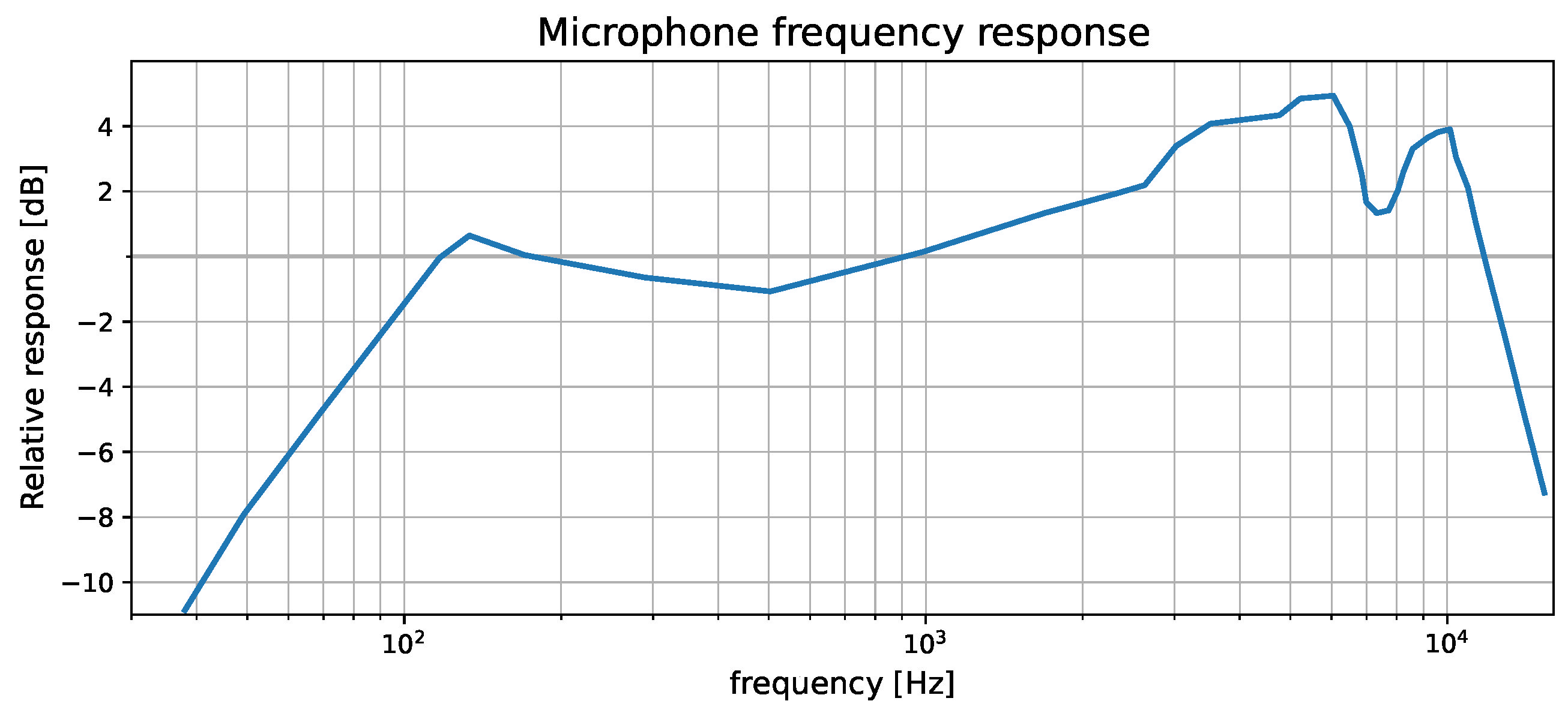
As smartphones are very common, use of such a microphone allows the proposed solution to be used in various environments, with a low-cost entry point. This is particularly relevant for potential in-field diagnostics, as smartphones can be a cheap computing platform. The possible frequency response of the microphone used in the above-mentioned study had a defined range of 20–20,000 Hz, as shown on the graph in Figure 5, its sensitivity was −42 dB, and the smartphone was positioned 0.4 m above the electric devices. The obtained acoustic data (saved as single channel, 44.1 kHz sampling frequency) were then cut into one-second recordings.

3. Results

3.1. Computational Setup

The practical implementation of functional logistic regression in binary variant was based on and developed from a Python library for functional data analysis scikit-fda (https://fda.readthedocs.io/en/latest/index.html, accessed on 26 July 2022) . This library contains ready-to-use classes and methods for FDA purposes. The solutions are fully compatible with the scikit-learn (https://scikit-learn.org/, accessed on 26 July 2022) library, and can be used along with standard data analysis and machine learning implementations. The basic element of the library is the class FDataGrid, which is used to represent functional data as a set of curves discretised in a grid of points. Other commonly used representations are FDataBasis or BSpline, which is used later in this paper. Both store data as the coefficients of functions. The library implements an exploratory analysis package which deals with techniques for summarizing, interpreting, and visualizing functional data. Plotting methods are fully compatible with the widely used Matplotlib. Another module contains scikit-learn machine learning algorithms implemented in versions compatible with functional data. The library stores example datasets, such as the Berkeley growth study and Canadian weather data, allowing users to understand FDA basics and implement methods. The web page is full of examples as well, along with API references and tutorials.

The multiclass variant of logistic regression was not stored in the scikit-fda library; instead, it was made from scratch based on an available binary version and on solutions for classical approaches stored in scikit-learn. The final proposed implementation is now stored as a public, open-source GitHub repository. The repository contains a demonstration with use of mock data and practical use based on actual data.

The database used for practical tests and visualizations contains voice recordings of commutator motors, both damaged and undamaged. More information about the data can be found in [15].

3.2. Common Preprocessing

The process flow (Figure 6) was prepared for the existing dataset of one-second voice recordings, although this could be easily changed to cover other examples. The flow starts by loading the data as a discrete time series of recorded samples, which are then transformed by fast Fourier transformation and normalized to the form of discrete functions of frequency with values between 0 and 1. Normalization is performed as follows:

$$x_{iN}\left(f\right)=\frac{x_i\left(f\right)-min\left(x\left(f\right)\right)}{max\left(x\right(f\left)\right)-min\left(x\right(f\left)\right)}$$

(14)

where $x\left(f\right)$ is a particular whole sample vector, $x_i$ is an i-th value of a vector, and $x_{iN}$ is a normalized value.

The frequency range is limited by the voice recording device, which in this case covers half of the sample rate, which is 44,100 Hz due to aliasing issues. An example of preprocessing is presented in Figure 7.

3.3. Binary Variant

For the binary variant, any two labels can be used. In the demo, recordings of two groups of damaged motors are chosen: those with two damaged gear teeth and those with five damaged teeth. To keep the visualization clear, the plots in this subsection cover only three samples from the dataset.

The prepared data are then transformed into a functional dataset using basis spline data approximation. In the example, 45 basis functions of the fourth order are used. The values are found experimentally, and might strongly depend on the analyzed data. Due to the dataset being limited to 30 recordings per group, 60 separate functions were prepared. Example is given in Figure 8.

Such approximation causes the dynamics of the data to be partially lost, although the samples’ features are retained. Ready-to-use functional data are then used in a binary functional logistic regression model fitting process, which is analogous to the classical discrete version known, for example, from machine learning algorithms. The dataset is split into training and validation subsets. Thereafter, the model is taught on training data, trying to fit the coefficients to attain the best accuracy. The final model score is obtained on the validation subset, which is unknown to the model during the fitting process. Exapmple of spline representation clasification is presented in Figure 9.

For the dataset of two groups of motors, the model accuracy is up to 88 percent; see Figure 10. The result depends heavily on the dataset splitting method due to the small size of the dataset. Populating data could increase the model’s stability.

3.4. Multiclass Variant

The multiclass variant is suitable for three or more labels. Implementation was tested on three separate classes of motor damage: one broken gear tooth, two broken teeth, and five broken teeth, each class containing 30 voice recordings.

The way in which data are transformed into functional basis spline functions remains the same as in binary variant. Due to the need to choose one of three classes, 90 functions are created, each containing information about a different voice recording.

Prepared and labeled data are used in the multiclass functional logistic regression model in a similar way as in the binary variant, and the dataset is again split into training and validation subsets with the same proportions (Figure 11). After the fitting process, the model gains around 67 percent accuracy when tested on the validation subset. The result again depends on the splitting method due to the small size of the dataset. Small size causes the classifier to sometimes become stacked on local minimums, which leads it to calculate wrong coefficients.

Confusion matrices (Figure 12) present results for different split methods, that is, for training and validation subsets containing different samples. The first is made for the same subsets as the plot above. The following five matrices show the results for different subsets obtained via different seed numbers used in the splitting method.

4. Discussion and Conclusions

In this analysis, we have used FDA and logistic (and softmax) regression classifiers as a proof of concept for fault recognition. As can be seen, this requires less computation and storage and can work very well.

As found in [15], the correlation between type of damage and acoustic response is significant. While preparing samples, it is very important to maintain a similar environment (distance between measured tool and microphone, etc.) and use the same device, such as a microphone. Possible additional samples should be recorded with the same microphone as well. As long as all samples are recorded by the exact same microphone and in a similar environment, the results should not differ excessively.

Basis spline approximation can prevent data from losing important features while simultaneously allowing data size to be reduced. A crucial factor is the number of spline functions used. Too few splines will result in losing major features of recorded data, while too many splines will extend the calculation and model fitting time and increase the size of the data.

The main advantage of the FDA approach is the ability to consider the entire frequency response, not just individual points, which is popular in harmonic analysis, for example, as it allows for comparison of individual profiles without dimension reduction provided by spline representation. One drawback is the introduction of averaging to frequency response caused by least squares, although this can be alleviated by first using a frequency response estimator.

As shown in Figure 12, the problem addressed here is sensitive to smaller datasets. This is an issue that will be covered in our future work. In particular, we are interested in extending the classifier into a Bayesian setting. Our previous results for Bayesian FDA show great promise, allowing missing data to be compensated for with prior knowledge and probabilistic modeling (see [16]). We intend to consider verification for other types of data as well.

References

- Ramsay, J.O.; Silverman, B.W. Functional Data Analysis; Springer: Berlin/Heidelberg, Germany, 2005. [Google Scholar]
- Ramsay, J.O. When the data are functions. Psychometrika 1982, 47, 379–396. [Google Scholar] [CrossRef]
- Ramsay, J.O.; Dalzell, C.J. Some Tools for Functional Data Analysis. J. R. Stat. Soc. Ser. B (Methodol.) 1991, 53, 539–561. [Google Scholar] [CrossRef]
- Besse, P.; Ramsay, J. Principal components analysis of sampled functions. Psychometrika 1986, 51, 285–311. [Google Scholar] [CrossRef]
- Pezzulli, S.; Silverman, B. Some Properties of Smoothed Principal Components Analysis. Comput. Stat 1993, 8, 1–16. [Google Scholar]
- Mousavi, S.N.; Sørensen, H. Functional logistic regression: A comparison of three methods. J. Stat. Comput. Simul. 2018, 88, 250–268. [Google Scholar] [CrossRef]
- Bueno-Larraz, B.; Berrendero, J.R.; Cuevas, A. On functional logistic regression: Some conceptual issues. arXiv 2018, arXiv:1812.00721. [Google Scholar]
- Denhere, M.; Billor, N. Robust Principal Component Functional Logistic Regression. Commun. Stat. Simul. Comput. 2016, 45, 264–281. [Google Scholar] [CrossRef]
- Ratcliffe, S.J.; Leader, L.R.; Heller, G.Z. Functional data analysis with application to periodically stimulated foetal heart rate data. I: Functional regression. Stat. Med. 2002, 21, 1103–1114. [Google Scholar] [CrossRef] [PubMed]
- Grenander, U. Stochastic processes and statistical inference. Ark. Mat. 1950, 1, 195–277. [Google Scholar] [CrossRef]
- Rao, C.R. Some statistical methods for comparison of growth curves. Biometrics 1958, 14, 1–17. [Google Scholar] [CrossRef]
- Wang, J.L.; Chiou, J.M.; Müller, H.G. Functional data analysis. Annu. Rev. Stat. Its Appl. 2016, 3, 257–295. [Google Scholar] [CrossRef] [Green Version]
- Patil, A.A.; Bovy, J.; Eadie, G.; Jaimungal, S. Functional Data Analysis for Extracting the Intrinsic Dimensionality of Spectra: Application to Chemical Homogeneity in the Open Cluster M67. Astrophys. J. 2022, 926, 51. [Google Scholar] [CrossRef]
- Rossi, F.; Delannay, N.; Conan-Guez, B.; Verleysen, M. Representation of functional data in neural networks. Neurocomputing 2005, 64, 183–210. [Google Scholar] [CrossRef] [Green Version]
- Glowacz, A. Recognition of acoustic signals of commutator motors. Appl. Sci. 2018, 8, 2630. [Google Scholar] [CrossRef] [Green Version]
- Baranowski, J.; Grobler-Dębska, K.; Kucharska, E. Recognizing VSC DC Cable Fault Types Using Bayesian Functional Data Depth. Energies 2021, 14, 5893. [Google Scholar] [CrossRef]