A Game-Theoretic Approach of Optimized Operation of AC/DC Hybrid Microgrid Clusters

Abstract

To maximize the benefits of microgrid clusters, a general model and analysis method for studying the optimized operation of AC/DC microgrid clusters using non-cooperative games is proposed. This paper first establishes the optimized objective function of an AC/DC microgrid for economic operations. Based on the supply and demand theory, the dynamic adjustment mechanism of electricity price is introduced into microgrid clusters, and a game model for the optimal operation of multiple microgrids is established. The Nash equilibrium solution of the established model is obtained by iterative search algorithm, and the convergence of the Nash equilibrium solution is also proven. Finally, the validity and economy of the proposed model are verified by the actual case.

1. Introduction

In order to solve the power quality impact of distributed energy on users and the power grid, a microgrid is introduced. The microgrid is both an independent power system and a power supply or a power-using unit in the power system. It can be divided into three structures according to the bus form: DC bus system, AC bus system, and AC/DC hybrid bus system [1]. An AC/DC microgrid can be compatible with both DC power and AC power, and the power system is convenient for the integration of different kinds of micro sources and loads [2], which is the main development direction of microgrids. Typical AC/DC microgrids include photovoltaic (PV) power generation, wind turbine (WT) generation, energy storage system (ESS), micro-gas turbine (MT) power generation and fuel cell (FC) power generation. The operation mode of an AC/DC hybrid microgrid mainly has two modes: islanding and grid-connected. One typical structure is shown in Figure 1.

An AC/DC microgrid cluster is composed of several AC/DC microgrids, which can improve the reliability of individual microgrids. The microgrid cluster is connected to large power grid through transformers. The whole microgrid cluster has a central controller, which is responsible for information collection and distribution among the microgrids and communication with the large power grid; it does not control the operating status of the micro-sources within each microgrid. Each microgrid is an independent individual with its own energy management system.

Microgrid clusters increase the complexity of system operation significantly; thus, the optimized operation of microgrids is critical to the economic benefits of the whole microgrid system. The optimized operation of microgrid clusters generally consists of model building and model solving while considering the economic, reliability, and environmental benefits of microgrid operation [3]. Gregoratti and Matamoros [4] uses a distributed Newton method and a consistency algorithm to provide the optimal control strategy to achieve the scheduling of the optimal economic operation of a microgrid cluster. However, this method ignores the problem of the existence of renewable prediction errors. Lee et al. [5] consider the impact of errors on the power system and use a random distribution function to simulate energy sources for optimal and economic operation between microgrids based on a centralized control approach. This approach suffers from communication delays and thus reduces the reliability of the system.

In order to reduce the operation cost and enhance the service reliability, Van-Hai Bui et al. [6] exploit the uncertainty of PV power generation and load and develop a joint scheduling model for multi-microgrid systems and grids based on opportunity constraints. The economic value has always been the main concern of the operation of microgrid clusters. Zhang et al. [7] consider the worst conditions of PV power generation and establish a two-stage robust optimization model. The model is solved using an optimization algorithm generated by column constraints, so as to reduce the operating costs of multi-microgrid systems. In Ref. [8], a two-layer interaction model is established. The model can achieve the economy of optimal day-ahead scheduling of the multi-micro network system using the node system. However, Refs. [6,7,8] only consider the optimal scheduling of microgrid clusters under the condition of source-load uncertainty. The different interests of each microgrid and the interaction between microgrids are ignored.

In a microgrid cluster, each microgrid belongs to different interest subjects. The above literature only considers the economic factors of microgrid cluster operation and the balance of interests between microgrids is ignored, which is contrary to the development trend of microgrids. Therefore, in order to improve the autonomy and intelligence of each microgrid individual and balance the multi-interest subjects, game theory becomes an important tool and method in the field of electric power.

Wei et al. [9] proposes a strategy of microgrid clustering based on the cooperative game, which can effectively reduce the regional network loss. However, this microgrid clustering approach under this coalition game will increase the cost to users. To guarantee the economic stability of the multiple microgrids system, a fair profit sharing among microgrids is needed. Compared with the cooperative game, non-cooperative games can optimize the operation of each microgrid while ensuring the benefits of the system.

In Ref. [10], based on a non-cooperative game, an energy pricing model for a smart distribution network containing multiple microgrids is developed. This model rationalizes energy pricing among multiple microgrids and improves the economic stability of the system. In order to maximize the benefits between microgrid clusters, individual microgrids and customers, the Stackelberg game theory is studied in [11]. An energy trading model and solving algorithm between microgrid clusters, individual microgrids and customers are developed, and a distributed algorithm is used to optimize the customers’ electricity consumption strategy according to the selling price of the microgrid. Mondal, Misra and Obaidat [12] establishs a game model for microgrids and users based on the Stackelberg game theory. The microgrid is the dominant player that maximizes its economic benefits through generation and optimal tariffs, and the user is the follower that determines the electricity demand model to achieve increased its own overall revenue. However, this model suffers from energy supply delays and require intensive user information to optimize the energy distribution.

To optimize the energy distribution, refs. [13,14] divide each microgrid into two categories of consuming and providing electricity. The energy flow problem among different microgrids is modeled as a game problem, in which each microgrid can optimize its own operation to maximize benefits. However, refs. [13,14] only consider the self-interest of the microgrid and the overall benefit of the microgrid group. In order to simplify non-cooperative game model, ref. [15] establishes a price setting mechanism for the transactions between multiple microgrids based on a potential game theory and investigates the benefits to the power suppliers and users under an open market. The above non-cooperative game has the problem of the benefit losses caused by multiple microgrids in the competition. AC/DC microgrid clusters are modeled as a two-level optimization problem using non-cooperative game theory and robust optimization methods in [16]. The two-level mathematical optimization model converts the model-solving process into a mathematical planning problem with Mathematical Programs with Complementarity Constraints (MPCC) via the Karush–Kuhn–Tucker (KKT) condition. The solving process is still complex, and many factors such as the environmental benefits and system converter losses are omitted in the optimization objective function.

This paper proposes an optimized operation strategy based on non-cooperative game theory, and each microgrid can maximize its own benefits while achieving a high overall return. The main contributions of this paper are as follows:

(1)

This paper proposes a novel potential game to achieve the optimized operation of AC/DC microgrid clusters. The benefit losses caused by multiple microgrids in the competition are reduced to a significantly low level. The existence and convergence of the Nash equilibrium of the proposed strict potential game have been proven.

(2)

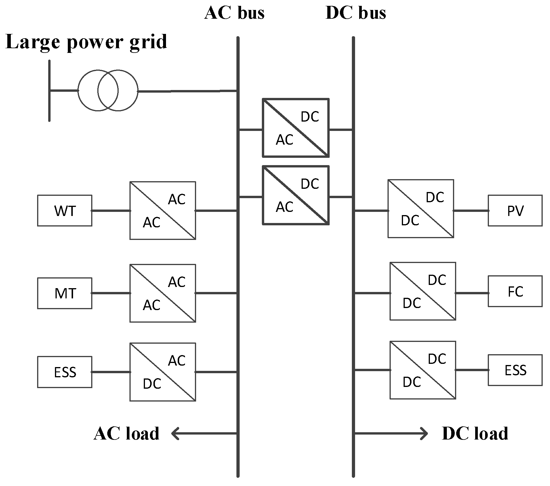
This paper introduces a new interlinking bidirectional AC/DC converter unit in the modeling of the microgrid.

(3)

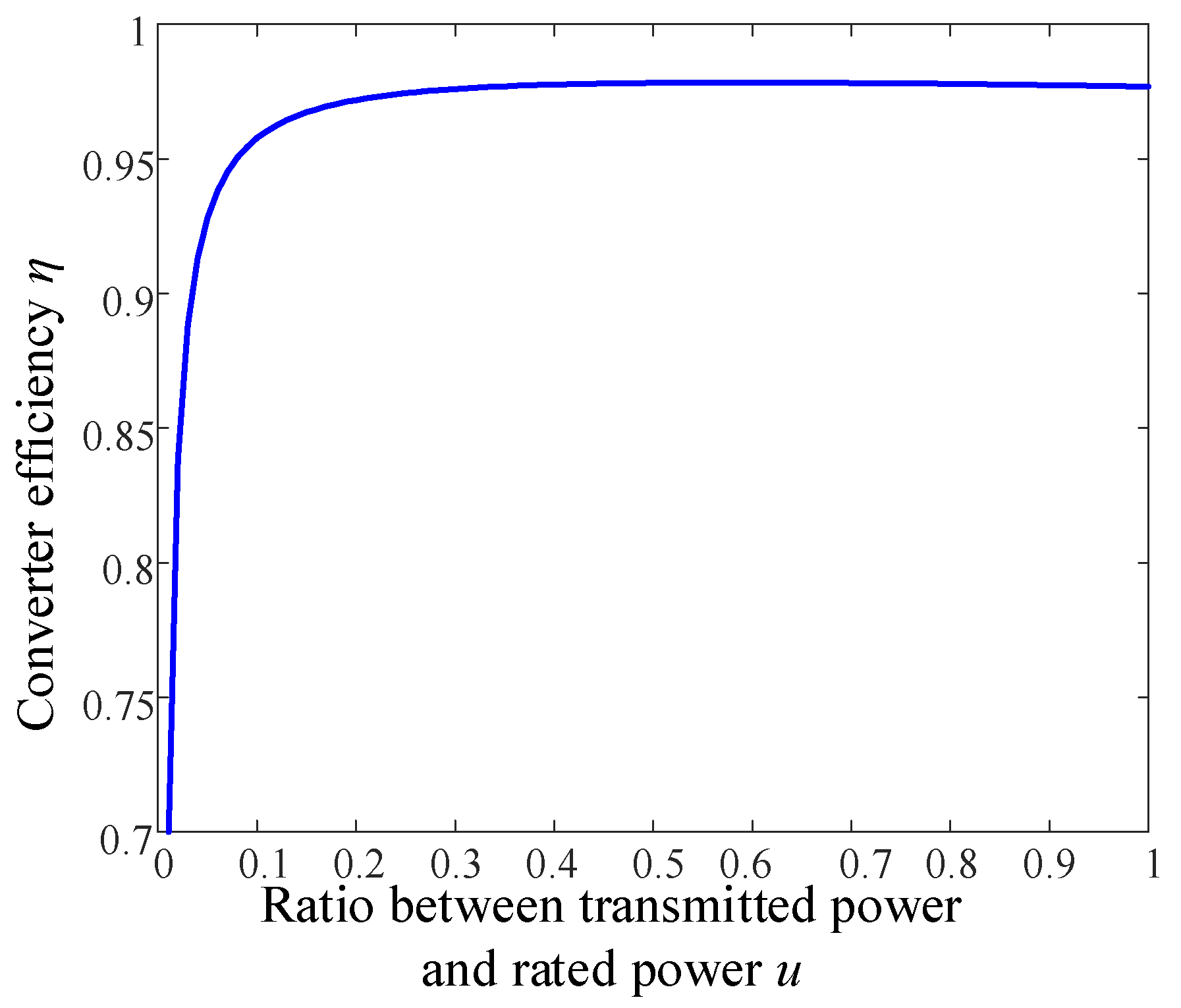
A new multiple objective optimization function has been introduced, which incorporates fuel cost, environmental cost, equipment maintenance cost, the transaction cost, and the equivalent cost of power loss in the interlinking converters.

(4)

Based on the supply and demand theory, the dynamic adjustment mechanism of electricity price is introduced into microgrid clusters.

(5)

The proposed potential game approach can transform the multivariate multi-objective optimization process into a process of finding the extreme value of the potential function, which simplifies the algorithm compared with Ref. [17].

2. Mathematical Model of AC/DC Hybrid Microgrid

2.1. Mathematical Models of Distributed Units

AC/DC hybrid microgrid includes a variety of distributed units. The mathematical models are established in this section. PV and WT generation are randomly affected by factors in the natural environment, such as illumination and wind speed, and belong to uncontrollable power sources under the maximum power output mode. MT, ESS, FC are controllable power sources. Therefore, these devices can be expressed by specific models, which belong to controllable power supplies. The bidirectional AC/DC converter is critical interlinking between AC grid and DC grid, which has been modeled here as well. The following is the mathematical model and analysis of the main equipment in the AC/DC hybrid microgrid.

(1) The output power of the WT system depends on the changes in wind speed. The wind speed probability density function based on the Weibull Distribution is expressed as:

$$f\left(v\right)=\frac{k}{c}{\left(\frac{v}{c}\right)}^{\mathrm{k}-1}exp\left[-{\left(\frac{v}{c}\right)}^{\mathrm{k}}\right]$$

(1)

where f is the probability density function of the Weibull Distribution; v is the wind speed; c is the scale parameter; and k is the shape parameter [18].

When the wind turbine is in operation, the rated wind speed, cut-out wind speed and start-up wind speed are several crucial factors affecting the output power of the fan. The power output mathematical model of WT generation is:

$$P_{\mathrm{WT}}=\{\begin{array}{l}0,\hspace{1em}\hspace{1em}\hspace{1em}\hspace{1em}\hspace{1em}\hspace{1em}v\le v_{\mathrm{ci}}\\ a_{\mathrm{WT}}{v}^2+b_{\mathrm{WT}}v+c_{\mathrm{WT}},\hspace{1em}{v}_{\mathrm{ci}}\le v\le v_{\mathrm{r}}\\ P_{\mathrm{r}\_\mathrm{WT}},\hspace{1em}\hspace{1em}\hspace{1em}\hspace{1em}{v}_{\mathrm{r}}\le v\le v_{\mathrm{co}}\\ 0,\hspace{1em}\hspace{1em}\hspace{1em}\hspace{1em}\hspace{1em}\hspace{1em}v\ge v_{\mathrm{co}}\end{array}$$

(2)

In Formula (2), a_WT, b_WT, and c_WT are coefficients of the fan. P_{r_WT} is the rated output power of the WT plant; P_WT is the actual output power; v and v_r represent the actual wind speed and the rated wind speed of the fan; v_ci and v_co represent the start-up wind speed and the cut-out wind speed of the fan.

(2) The grid-connected PV system is generally composed of three parts: PV array module, grid-connected inverter/converter and controller [19]. The characteristic function of PV cell output power is expressed as:

$$P_{\mathrm{PV}}=P_{\mathrm{STC}}\frac{G_{\mathrm{ING}}}{G_{\mathrm{STC}}}\left(1+K\left(T_{\mathrm{c}}-T_{\mathrm{r}}\right)\right)$$

(3)

where G_STC is the irradiation intensity under the test conditions (ambient temperature is 25 °C, 1000 W/m²); G_ING is the actual irradiation intensity in W/m²; K is the power temperature coefficient in ppm/°C; T_r is the reference temperature; T_c is the actual temperature; P_STC is the maximum output power for standard tests in kW; and P_PV is the actual output power in kW [20].

(3) MT is generally used as a backup power generation device in the microgrid. MT has the advantages of high efficiency, small volume, convenient installation and simple maintenance. The functional relationship between the energy output and fuel cost of MT can be expressed as follows when the natural gas is employed as the fuel:

$$F_{\mathrm{fuel},\mathrm{MT}}\left(t\right)=\frac{C_{\mathrm{fuel}}}{Q_{\mathrm{LHV}}}\sum _t\frac{P_{\mathrm{MT}}\left(t\right)}{{\eta }_{\mathrm{MT}}\left(t\right)}\Delta T$$

(4)

where C_fuel is the unit price of natural gas; Q_LHV is the low calorific value of natural gas; ΔT is the unit period; P_MT is the actual output power of the MT in kW; η_MT is operating efficiency.

(4) FC is a kind of clean distributed energy, which has the advantages of high energy conversion efficiency, fuel diversification, small footprint, short construction cycle, low or zero emissions, and so on [21]. The functional relationship between energy output and fuel cost of FC is as follows when the natural gas is employed as the fuel:

$$F_{\mathrm{fuel},\mathrm{FC}}\left(t\right)=\frac{C_{\mathrm{fuel}}}{Q_{\mathrm{LHV}}}\sum _t\frac{P_{\mathrm{FC}}\left(t\right)}{{\eta }_{\mathrm{FC}}\left(t\right)}\Delta T$$

(5)

where C_fuel is the unit price of natural gas; P_FC is the output power; Q_LHV is the low calorific value of natural gas; and η_FC is the generating efficiency of the FC. Normally, the generating efficiency of FC can be expressed as:

$${\eta }_{\mathrm{FC}}\left(t\right)=a_1{P}_{\mathrm{FC}}\left(t\right)/P_{\mathrm{FC},max}+a_2$$

(6)

where P_FC,max is the rated output power of the FC; a₁ and a₂ are the constant coefficient related to the FC device.

(5) ESS plays the role of improving the power quality, short-term power supply backup and energy buffer in the microgrid. Among them, battery ESS, pumped ESS and other equipment are widely used. In this paper, the commonly used lead-acid battery is used as the microgrid ESS. The operating cost function of the battery is:

$$F_{\mathrm{ESS}}(t)=\beta \cdot P_{\mathrm{ESS}}(t)+C_{\mathrm{cycle}}(t)$$

(7)

where F_ESS(t) is the operating cost of the battery during the t period; P_ESS(t) is the charging and discharging power of the battery; β is the operating maintenance factor of the battery; C_cycle(t) is the cost of charge and discharge loss of the battery.

The state of the battery in operation can be expressed by SOC (State of Charge). The expressions of SOC during charging and discharging are:

While the battery is being charged:

$$S_{\mathrm{soc}}(t)=S_{\mathrm{soc}}(t-1)+P_{\mathrm{ESS}}(t){\eta }_{\mathrm{ESS}1}\Delta T,P_{\mathrm{ESS}}(t)\le 0$$

(8)

While the battery is discharging:

$$S_{\mathrm{soc}}(t)=S_{\mathrm{soc}}(t-1)+\frac{P_{\mathrm{ESS}}(t)}{{\eta }_{\mathrm{ESS}2}}\Delta T,P_{\mathrm{ESS}}(t)\ge 0$$

(9)

where S_soc(t) is the charge of the battery at t; s(t) is the charge and discharge power at t, with discharge direction as the positive direction; P_ESS(t) ≤ 0 represents the charging power, and P_ESS(t) ≥ 0 represents the discharging power.

In addition, the capacity constraint and power constraint of the battery are as follows:

$$\{\begin{array}{l}{E}_{\mathrm{ESS}}{}_{,\min }\le E_{\mathrm{ESS}}(t)\le E_{\mathrm{ESS}}{}_{,\max }\\ P_{\mathrm{ESS}}{}_{,\min }\le P_{\mathrm{ESS}}(t)\le P_{\mathrm{ESS}}{}_{,\max }\end{array}$$

(10)

where E_ESS,min and E_ESS,max are the upper and lower limits of the battery capacity, and P_ESS,min and P_ESS,max are the upper and lower limits of the battery output power.

(6) AC/DC bidirectional converter is used to connect the AC and DC subgrid of the AC/DC hybrid microgrid by controlling the power flow between the AC bus and the DC bus. It plays an important role in voltage stability and power balance of the system. According to the demand for the flow of electrical energy, the bidirectional converter is working in rectification state or inverter state. The typical efficiency curve expression of a bidirectional converter can be approximately expressed as:

$$\eta =c_{1}u+c_2+c_3/u$$

(11)

In Formula (11), c₁~c₃ are constant coefficients under certain conditions; u is the ratio between the transmission power and the rated power of the converter. In this paper, the fitting coefficient are c₁ = −0.0087, c₂ = 0.9886 and c₃ = −0.003. The converter efficiency curve is shown in Figure 2.

2.2. Mathematical Model of the AC/DC Hybrid Microgrid

The optimal operation of microgrid refers to the microgrid operation scheduling plan according to the established optimization objective function and constraint conditions. It is made by the energy management system according to the operation status of each power source in the microgrid, user load prediction and power market. The optimization objective function in this paper mainly considers the fuel cost of power generation, operating maintenance cost, environmental pollution conversion cost, converter power loss and other factors used in the AC/DC hybrid microgrid. It mainly includes the following parts:

(1) Fuel cost

The function expression of total fuel cost F_fuel:

$$F_{\mathrm{fuel}}={\displaystyle \sum _M{F}_{\mathrm{MT}}+}{\displaystyle \sum _N{F}_{\mathrm{FC}}}$$

(12)

In Formula (12), F_FC and F_MT are the fuel cost consumed by the FC and MT in the microgrid; M is the number of MTs in the microgrid, and N is the number of FC power generation devices in the microgrid.

(2) The cost of electricity transaction

This refers to the cost of electricity purchased or sold between microgrid and large power grid (or other microgrid clusters), which is related to the electricity price of the external grid and the power exchanged. The calculation formula is:

$$F_{\mathrm{buy}}={\displaystyle \sum _{t=1}^T[P_{\mathrm{MG}}(t)B_{\mathrm{S}}(t)(1-\sigma )}+P_{\mathrm{MG}}(t)B_{\mathrm{P}}(t)\sigma ]$$

(13)

where

$$\sigma =\{\begin{array}{l}0,\hspace{1em}{P}_{\mathrm{MG}}<0\\ 1,\hspace{1em}{P}_{\mathrm{MG}}>0\end{array}$$

In Formula (13), P_MG(t) is the electricity transaction by the microgrid during period t; P_MG(t) > 0 represents the microgrid sells electricity outward; P_MG(t) < 0 represents the microgrid purchases electricity. B_P(t) and B_S(t) are the unit purchase price and the unit sale price of electricity during the period t.

(3) Operating maintenance costs

The calculation formula for the operating maintenance cost of each equipment in the microgrid is:

$$F_{\mathrm{om}}={\displaystyle \sum _{t=1}^T{\displaystyle \sum _{i=1}^{N_{\mathrm{G}}}{k}_{\mathrm{omi}}}{P}_{\mathrm{i}}(t)}$$

(14)

In Formula (14), N_G is the number of power units in the AC/DC hybrid microgrid; k_omi is the operating maintenance cost coefficient of the equipment; P_i(t) represents the output power of the power generation unit i. The maintenance cost coefficient of distributed power supply in the microgrid is shown in

Table 1. Maintenance cost coefficient for different equipment.

Device Type	Maintenance Cost (CNY/kW)	Device Type	Maintenance Cost (CNY/kW)
MT	0.03992	PV array	0.0096
FC	0.02849	WT	0.0296

.

(4) Environmental cost

MT and FC will emit CO₂, SO₂, NO_x and other pollutants in the process of power generation. Considering comprehensively the emission of polluting gases from each micro-source and the treatment cost of polluting gases, the mathematical expression of environmental conversion cost is:

$$F_{\mathrm{en}}={\displaystyle \sum _{t=1}^T{\displaystyle \sum _{i=1}^N{\displaystyle \sum _{j=1}^M{\mu }_j}{E}_{i,j}}{P}_i(t)}$$

(15)

In Formula (15), N is the number of distributed generation power sources, and M is the number of pollutant types; μ_j and E_ij are the environmental evaluation coefficient and emission factor of different types of pollutants, respectively.

Table 2. Pollutant emission (g/kWh).

Generating Equipment	CO2	NOx	SO2
MT	730	0.62	0.001
FC	360	0.25	0.00
PV	0.00	0.00	0.00
WT	0.00	0.00	0.00

shows the emissions of different types of pollutants from various distributed power sources [22]; P_i(t) is the output power of the power source i.

(5) The equivalent cost of power loss in the interlinking converters

The power loss cost of the converters mainly considers the power loss through the bidirectional converter when power is exchanged between the DC and AC subgrids. The calculation formula is as follows:

$$F_{\mathrm{Loss}}={\displaystyle \sum _{t=1}^T\alpha (t)P_{\mathrm{Loss}}(t)}$$

(16)

where

$$P_{\mathrm{Loss}}(t)={\displaystyle \sum _{q=1}^{N_q}(1-{\eta }_q)\left|P_q(t)\right|}$$

(17)

In Formula (16), α(t) is the electricity price of the power grid in period t; P_Loss(t) is the power loss of converter in t; N_q is the number of bidirectional converters in the microgrid; η_q is the working efficiency of converter q; P_q(t) is the power that flows through the bidirectional converter during period t.

In conclusion, the expression for the optimization objective function constructed in this paper is:

$$\min F={\displaystyle \sum _{t=1}^T\{{\displaystyle \sum _{i=1}^{N_G}[K_i{P}_i(t)+{\displaystyle \sum _{j=1}^M{\mu }_j{E}_{i,j}}{P}_i(t)+k_{omi}{P}_i(t)]+}\alpha (t)P_{\mathrm{MG}}(t)+\alpha (t)P_{\mathrm{Loss}}(t)\}}$$

(18)

In Formula (18), T is the number of total optimization calculation periods; P_i(t) is the power output of power source I in period t; N_G is the number of distributed generation units; power generation units include WT, PV, MT and FC; K_i for the i-th generator fuel cost factor; k_omi is the i-th generation source operating maintenance factor; μ_j and E_ij are environmental evaluation standard and pollutant emission coefficient, respectively; P_Loss(t) is the power loss of converter in t; α(t) is the price of large power network in t; P_MG(t) is the electricity purchased or sold by the microgrid during the t period; the coefficient of fuel cost and environmental cost of WT and PV are zero.

The optimal operation of the microgrid should optimize the dispatching of the power output of the power generation sources and ESS, which is based on the premise that the power balance of the system, the safe operation of the equipment and the quality of power supply to the customers are guaranteed.

(1) Constraint on the output power of each generating equipment.

$$P_i{}^{\min }\le P_i(t)\le P_i{}^{\max }$$

(19)

In Formula (19), P_i^min represents the lower limit of the output power; P_i^max represents the upper limit of the output power.

(2) Constraint on the power of grid-connected contact line

$$0\le P_{\mathrm{buy}}(t)\le P_{\mathrm{buy}}^{\max }$$

(20)

In Formula (20), P_buy^max is the upper limit of the power that microgrids can purchase from the main grid.

(3) Constraint on capacity of the battery and charging and discharging power of the battery

$$\{\begin{array}{l}{E}_{\mathrm{ESS}}{}_{,\min }\le E_{\mathrm{ESS}}(t)\le E_{\mathrm{ESS}}{}_{,\max }\\ P_{\mathrm{ESS}}{}_{,\min }\le P_{\mathrm{ESS}}(t)\le P_{\mathrm{ESS}}{}_{,\max }\end{array}$$

(21)

In Formula (21), E_ESS,min is the minimum remaining charge of the battery. The value in this paper is set as 10% of the rated capacity; E_ESS,max is the maximum remaining charge of the battery. The value in this paper is set as 90% of the rated capacity; P_ESS,min and P_ESS,max are the minimum and maximum charge and discharge power of the battery.

(4) Constraint on the number of times that the battery can be charged and discharged

$${\displaystyle \sum _{t=1}^T{\lambda }_t}\le {\lambda }_{\max }$$

(22)

In the formula, λ_t is the state of the battery at time t, when λ_t = 1, the battery is in the charge and discharge state; λ_max is the rated maximum permissible number of charges and discharges of the battery.

(5) Minimum start/stop time constraint

$$\{\begin{array}{l}{T}_{\mathrm{on}}\ge T_{\mathrm{on}}^{\min }\\ T_{\mathrm{off}}\ge T_{\mathrm{off}}^{\min }\end{array}$$

(23)

In Formula (23), T_on^min and T_off^min are the minimum continuous start time and stop time for the MT respectively.

(6) Constraints on real-time power balance of the system

$${\displaystyle \sum P_i(t)}+P_{\mathrm{buy}}(t)+P_{\mathrm{ES}}(t)=P_{\mathrm{Load}}(t)+P_{\mathrm{Loss}}(t)$$

(24)

Constraints on AC regional power balance

$${\displaystyle \sum P_{i,\mathrm{AC}}(t)}+P_{\mathrm{buy}}(t)+P_{\mathrm{ESS},\mathrm{AC}}(t)=P_{\mathrm{Load},\mathrm{AC}}(t)+P_{\mathrm{Loss},\mathrm{AC}}(t)+P_{\mathrm{Loss},\mathrm{AC}}(t)$$

(25)

Constraints on DC regional power balance

$${\displaystyle \sum P_{i,\mathrm{DC}}(t)}+P_{\mathrm{buy}}(t)+P_{\mathrm{ESS},\mathrm{D}C}(t)=P_{\mathrm{Load},\mathrm{DC}}(t)+P_{\mathrm{Loss},\mathrm{DC}}(t)$$

(26)

In Formula (26), P_i(t), P_i,AC(t), and P_i,DC(t) are the output power, output AC power, and output DC power of the i-th power source respectively; P_buy(t) is the electricity purchased from the large power grid during period t; P_ESS(t) is the charge and discharge power of the battery during period t; P_con(t) is the active power passing through the converter from the AC side to the DC side during period t; P_Loss(t) is the active power loss during period t; P_Load(t) is the total amount of load demand within the microgrid during period t. In the above variables, subscript AC and DC represent AC power and DC power, respectively.

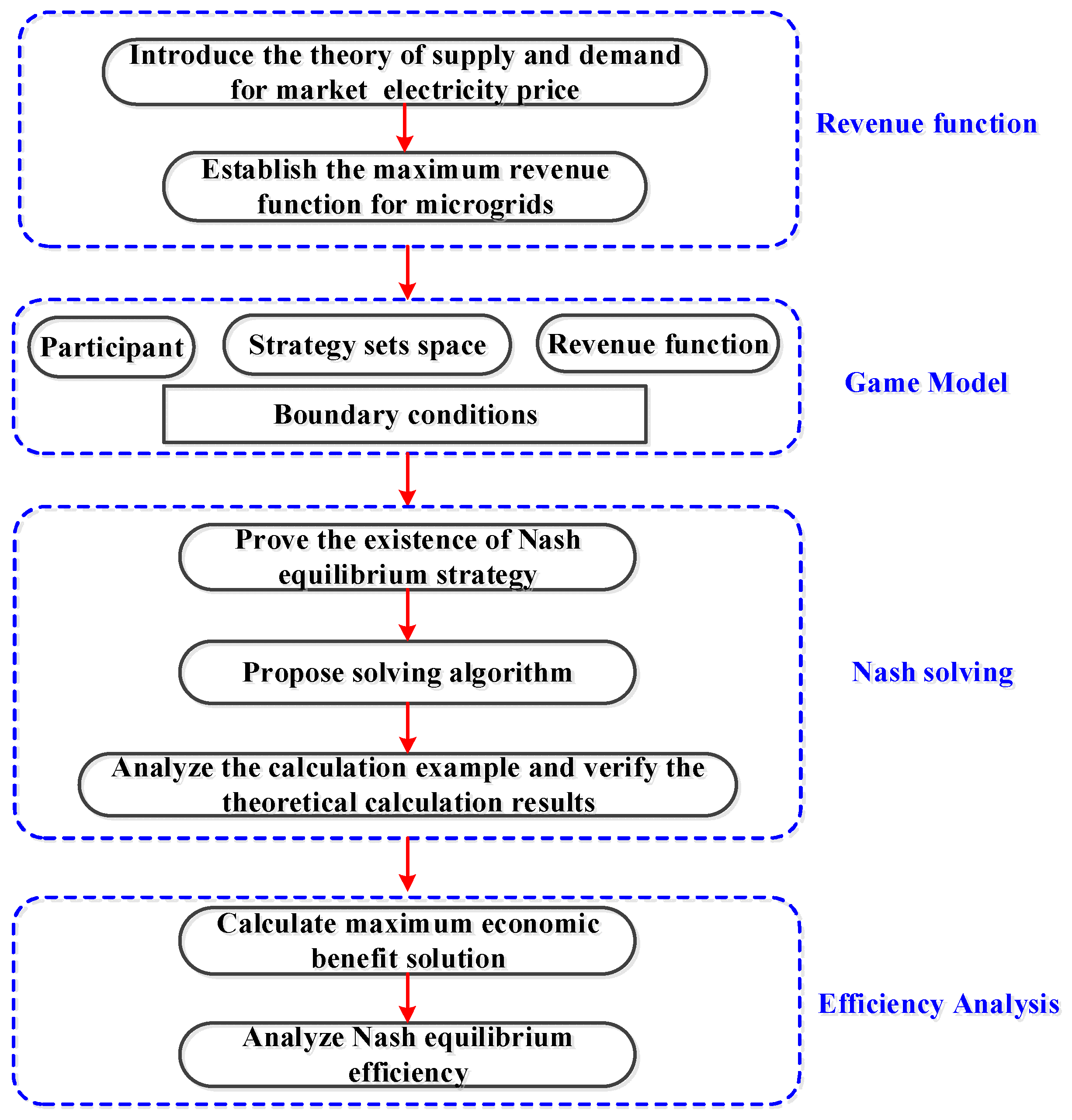
2.3. Optimized Revenue Function for Microgrids Based on Supply and Demand Theory

The transaction electricity price in the microgrid can be described by a linear supply and demand theory widely adopted for most electricity markets, with the functional expression as

$$a(t)=a_0(t)-b(t){\displaystyle \sum _{n\in N}{P}_n(t)}$$

(27)

a₀(t) is the base electricity price of the large power grid at time t.

b(t) is the price multiplier, a parameter that describes the relationship between the electricity price and the supply and demand.

a(t) is the transaction electricity price at time t.

P_n(t) is the power output of microgrid n to the microgrid cluster in time period t.

N is the number of microgrids in the microgrid cluster.

In Equation (27), when P_n(t) > 0, it indicates that the microgrid n sells electricity in time period t; when P_n(t) < 0, it indicates that the microgrid n purchases electricity in time period t. b(t) is a coefficient greater than zero, so when ∑P_n(t) > 0, it indicates that the overall microgrid cluster is selling electricity at a lower price than the large power grid; when ∑P_n(t) < 0, it indicates that the overall microgrid cluster is purchasing electricity, and the transaction electricity price is greater than that of the large power grid.

The expression of the minimum cost function for microgrid operation in microgrid n based on fuel cost, equipment maintenance cost, converter power loss, environmental cost, and purchased power cost is

$$\min F_n=F_n(t)-{\displaystyle \sum a(t)P_n(t)}$$

(28)

where F_n(t) is the transaction cost function on the output power of the generation units within the microgrid n, including fuel costs, equipment maintenance costs, and environmental pollution discounting costs. With reference to Equation (18), the functional expression for F_n(t) is

$$F_n(t)={\displaystyle \sum _{t=1}^T\{{\displaystyle \sum _{i=1}^{N_G}[K_i{P}_i(t)+{\displaystyle \sum _{j=1}^M{\mu }_j{E}_{i,j}}{P}_i(t)+k_{\mathrm{omi}}{P}_i(t)]}}+a(t)P_{\mathrm{Loss}}(t)\}$$

(29)

where P_i(t) is the power output of the generation source I at time t; N_G is the number of distributed generation units in the microgrid; K_i is the fuel cost coefficient of the generation source i; K_omi is the maintenance coefficient of the generation source i; μ_j and E_i,j are respectively the environmental evaluation criteria and pollutant emission coefficients; P_Loss(t) is the power loss of the converter at time t; a(t) is the electricity price of the large power grid at time t.

Bringing Equation (27) into Equation (28), the revenue function of microgrid n can be obtained as Equation (30), where P_m(t) is the power output from other microgrid of the same microgrid cluster such as microgrid m to the microgrid cluster at time t. It can be seen that the revenue function of microgrid n is not only related to the output power of its own micro-source, but also related to the power emitted by other microgrids.

$$U_n=-\min F_n={\displaystyle \sum _{t\in T}[a_0(t)P_n(t)-b(t)P_n{(t)}^2-{\displaystyle \sum _{m\ne n,m\in N}b(t)P_m(t)P_n(t)}]-F_n(t)}$$

(30)

In operation, the generation units in the microgrid have to satisfy constraints based on Equations (8), (9) and (19)–(26). Each microgrid has to satisfy its own internal power balance condition expressed as

$$P_{\mathrm{PV}}(t)+P_{\mathrm{WT}}(t)+P_{\mathrm{MT}}(t)+P_{\mathrm{FC}}(t)+P_{\mathrm{ESS}}(t)=P_n(t)+P_{\mathrm{Load}}(t)+P_{\mathrm{Loss}}(t)$$

(31)

where P_PV(t), P_WT(t), P_MT(t), P_FC(t), P_ESS(t) are respectively the output power of PV, WT, MT, FC and ESS at time t; P_n(t) is the power output of the microgrid n to the microgrid cluster at time t; P_Loss(t) is the active power loss in converters at time t; P_Load(t) is the total load demand in the microgrid n at time t.

3. Optimal Operation of AC/DC Microgrid Cluster Based on Potential Game Theory

Figure 3 shows optimal operation process of microgrid cluster based on game theory. Based on the supply and demand theory, the revenue function of microgrids is established in the Section 2. The revenue functions of each microgrid are coupled with each other and the strategy sets are independent of each other. The game model for optimal operation of multiple microgrids is established. It is proved that the non-cooperative game model is a strict potential game, and then prove the existence and convergence of the Nash equilibrium solution. The Nash equilibrium solution is solved by iterative search method. Each microgrid maximizes its own benefit under the Nash equilibrium operation strategy. The maximum benefit of the microgrid cluster is solved, and the efficiency in Nash equilibrium condition is verified.

3.1. Non-Cooperative Game Model for Optimal Operation of Microgrid Clusters

From Equation (30), it can be seen that the revenue functions of each microgrid are coupled with each other and the strategy sets are independent of each other, and each microgrid maximizes the benefits through its own optimal operation. The optimal operation process of N microgrids can be formulated as a non-cooperative game. The game model of microgrids is Γ = {N, S, U}, where N is the participant set, S is the space composed of the strategy sets of N microgrids, and U is the revenue functions space. Taking the microgrid cluster containing three microgrids as an example, the game model based on the non-cooperative game is represented as follows.

(1) Participant set

The three microgrids in the microgrid cluster are denoted by MG1, MG2, and MG3, and the set of participants is noted as

$$N=\left\{\mathrm{MG}1,\mathrm{MG}2,\mathrm{MG}3\right\}$$

(32)

(2) Strategy sets space

The respective strategies of the three microgrids are the output power {P_PV, P_WT, P_MT, P_FC, P_MG, P_bat,ac, P_bat,dc} of each device in the microgrid, and the strategy variables can be taken continuously within the boundary conditions allowed by the devices, and the strategy sets space of each participant is denoted as

$$S=\left\{S_{\mathrm{MG}1},S_{\mathrm{MG}2},S_{\mathrm{MG}3}\right\}$$

(33)

(3) Revenue functions space

The revenue function is the economic benefit of each microgrid, including the transaction costs with the large power grid, fuel costs, environmental costs and equipment maintenance costs, and the equivalent cost of power loss in the interlinking converters, etc. The three microgrids are denoted as U_MG1, U_MG2 and U_MG3 respectively, and the revenue function of the game is thus

$$\begin{array}{l}{U}_{\mathrm{MG}1}=\left\{S_{\mathrm{MG}1},S_{\mathrm{MG}2},S_{\mathrm{MG}3}\right\}\\ U_{\mathrm{MG}2}=\left\{S_{\mathrm{MG}1},S_{\mathrm{MG}2},S_{\mathrm{MG}3}\right\}\\ U_{\mathrm{MG}3}=\left\{S_{\mathrm{MG}1},S_{\mathrm{MG}2},S_{\mathrm{MG}3}\right\}\end{array}$$

(34)

3.2. Proof of Existence of Nash Equilibrium Solution of Non-Cooperative Game Model

The potential game is a special form of non-cooperative game. The properties of the potential game ensure the existence of the Nash equilibrium solution based on the potential game model without the need for a tedious proof process [17].

Definition: If there exists a potential function Φ satisfying the following equation:

Φ: S→R, ∀ n∈N, ∀ x_−n∈S_−n, ∀ x_n, x^′_n∈S_n

$$\Phi (x_n^{\prime },x_{-n})-\Phi (x_n,x_{-n})=U_n(x_n^{\prime },x_{-n})-U_n(x_n,x_{-n})$$

(35)

This game model Γ is called a strict potential game, where N is the insider, U_n is the revenue function, and S_n is the set of strategies; x_n is the strategy of the participant n, i.e., the output power of the generation equipment in the microgrid n, and x_−n is the combination of strategies of the participants other than the participant n. x^′_n is another strategy of the participant n and x^′_−n is the combination of strategies of other participants in this condition.

Based on the microgrid revenue function in Equation (30), the potential function is as follows.

$$\Phi (x)={\displaystyle \sum _{t\in T}\{{\displaystyle \sum _{n\in N}[a_0(t)P_n(t)-b(t)P_n{(t)}^2]}}-b(t){\displaystyle \sum _{n\in N}{\displaystyle \sum _{m\in N}{P}_m(t)P_n(t)}}\}-{\displaystyle \sum _{n\in N}{F}_n(t)}$$

(36)

where T is the total number of time periods of the game model optimal operation. Then, Equation (36) satisfies the condition Equation (35). That is to say, the proposed game Γ = {N, S, U} is a strictly potential game. The existence of the Nash equilibrium solution of the proposed model and the convergence of the solution are guaranteed according to the properties of the potential game. At the same time, the use of the potential game can also convert the multi-objective optimization optimal operation into a single objective potential function searching the extreme value, which greatly simplifies the solving algorithm.

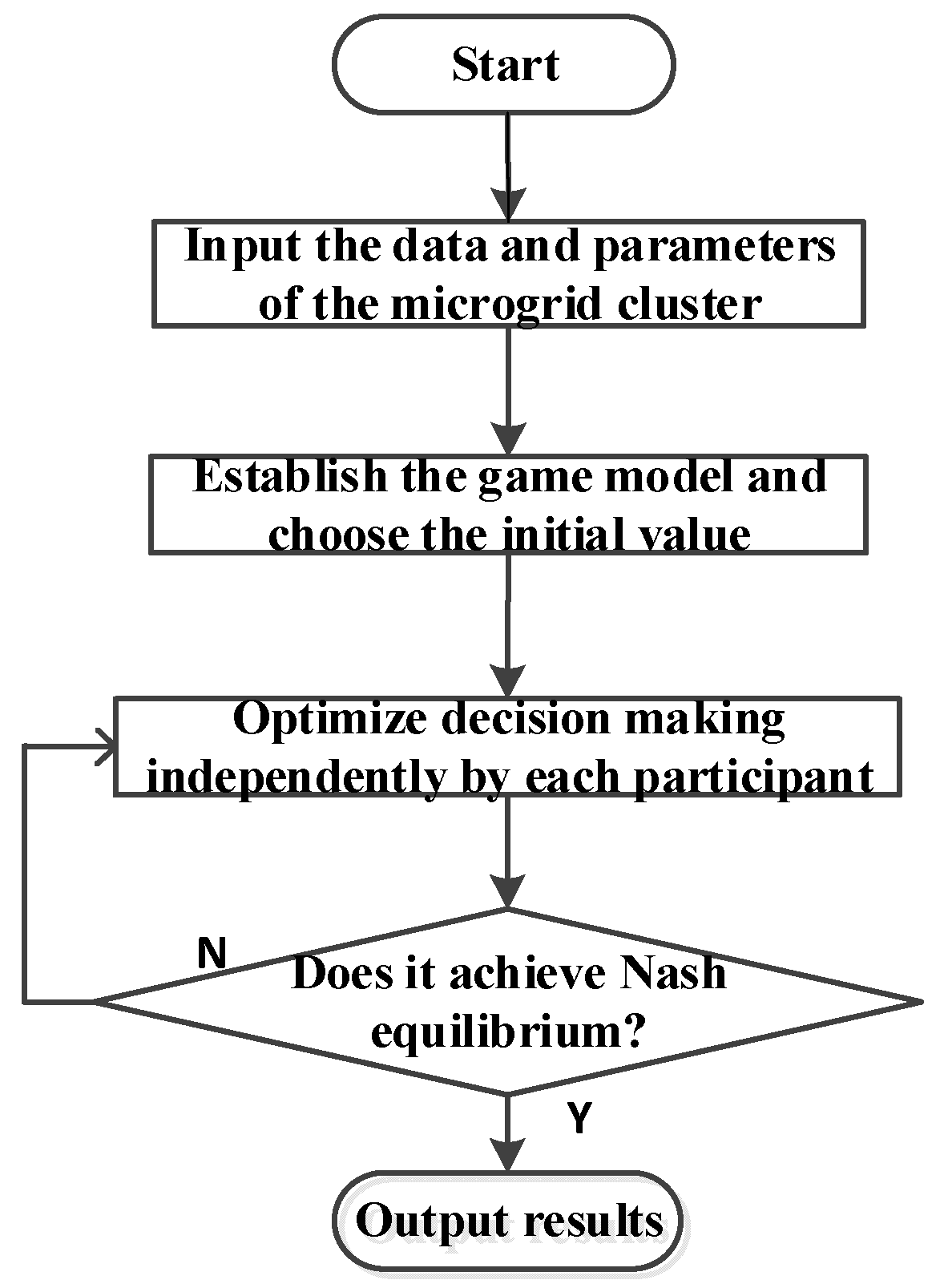
3.3. Solving Method for Nash Equilibrium Solution of Non-Cooperative Game Model

For the study of microgrid cluster optimized operation, this paper uses the iterative search method to solve the Nash equilibrium solution in Algorithm 1 and Figure 4, and the solving steps are as follows.

Step 1: input the technical data and parameters of the microgrid cluster. Input the parameters of distributed power sources in the microgrid, including wind speed and light intensity as well as grid base electricity price, load forecast, etc.

Step 2: establish the revenue functions U_MG1 = {S_MG1, S_MG2, S_MG3}, U_MG2 = {S_MG1, S_MG2, S_MG3}, U_MG3 = {S_MG1, S_MG2, S_MG3}, for the maximum benefit of each microgrid and the game model Γ = {N, S, U} for N microgrids.

Step 3: choose the initial value of the equilibrium point {P_PV(t), P_WT(t), P_MT(t), P_FC(t), P_MG(t), P_bat,ac(t), P_bat,dc(t)}. Here, the initial values are chosen randomly in the strategy space. Convergence to the Nash equilibrium is possible regardless of the initial value.

Step 4: each participant optimizes its own strategy independently. For example, in the optimization process of the round k, each participant makes an independent optimization decision based on the optimization result ($S_{\mathrm{MG}1}^{k-1}$, $S_{\mathrm{MG}2}^{k-1}$, $S_{\mathrm{MG}3}^{k-1}$) of the previous round k − 1 and obtains the strategy combination ($S_{\mathrm{MG}1}^k$, $S_{\mathrm{MG}2}^k$, $S_{\mathrm{MG}3}^k$) curated in the round k by the argmax decision rule.

$$\begin{array}{l}{S}_{\mathrm{MG}1}^k=\arg \underset{S_{\mathrm{MG}1}}{\max }{U}_{\mathrm{MG}1}(S_{\mathrm{MG}1},S_{\mathrm{MG}2}^{k-1},S_{\mathrm{MG}3}^{k-1})\\ S_{\mathrm{MG}2}^k=\arg \underset{S_{\mathrm{MG}2}}{\max }{U}_{\mathrm{MG}2}(S_{\mathrm{MG}1}^{k-1},S_{\mathrm{MG}2},S_{\mathrm{MG}3}^{k-1})\\ S_{\mathrm{MG}3}^k=\arg \underset{S_{\mathrm{MG}3}}{\max }{U}_{\mathrm{MG}3}(S_{\mathrm{MG}2}^{k-1},S_{\mathrm{MG}2}^{k-1},S_{\mathrm{MG}3})\end{array}$$

(37)

Step 5, determine whether the Nash equilibrium is reached based on the obtained optimal strategies. If the optimal strategies calculated adjacently are consistent, as in Equation (38), the strategy combination is indicated as a Nash equilibrium solution. If the Nash equilibrium is found, output the result ($S_{\mathrm{MG}1}^{*}$, $S_{\mathrm{MG}2}^{*}$, $S_{\mathrm{MG}3}^{*}$); otherwise, return to step 4 for further optimization decisions.

$$(S_{\mathrm{MG}1}^k,S_{\mathrm{MG}2}^k,S_{\mathrm{MG}3}^k)=(S_{\mathrm{MG}1}^{k-1},S_{\mathrm{MG}2}^{k-1},S_{\mathrm{MG}3}^{k-1})=(S_{\mathrm{MG}1}^{\ast },S_{\mathrm{MG}2}^{\ast },S_{\mathrm{MG}3}^{\ast })$$

(38)

Algorithm 1: Pseudocode of solving proposed game

Inputs: PFC,max, PFC,min, PMT,max, PMT,min, Pbat,ac,max, Pbat,dc,max, ηbat,ac, ηbat,dc, cbat,ac, cbat,dc, a0(t), b(t), PPV(t), PWT(t), PLoad(t), PPV,max, PWT,max, EESS,max; Outputs: ($S_{\mathrm{MG}1}^{*}$, $S_{\mathrm{MG}2}^{*}$, $S_{\mathrm{MG}3}^{*}$); 1. Decide random initial value: {PPV, PWT, PMT, PFC, PMG, Pbat,ac, Pbat,dc}∈{SMG1, SMG2, SMG3}; 2. Calculate: UMG1, UMG2, UMG3  while ($S_{\mathrm{MG}1}^k$, $S_{\mathrm{MG}2}^k$, $S_{\mathrm{MG}3}^k$) ≠ ($S_{\mathrm{MG}1}^{k-1}$, $S_{\mathrm{MG}2}^{k-1}$, $S_{\mathrm{MG}3}^{k-1}$) 3. $S_{\mathrm{MG}1}^k$=${}_{S_{\mathrm{MG}1}}^{\mathrm{argmax}}$ UMG1($S_{\mathrm{MG}1}$, $S_{\mathrm{MG}2}^{k-1}$, $S_{\mathrm{MG}3}^{k-1}$); 4. $S_{\mathrm{MG}2}^k$=${}_{S_{\mathrm{MG}2}}^{\mathrm{argmax}}$ UMG2($S_{\mathrm{MG}1}^{k-1}$, $S_{\mathrm{MG}2}$, $S_{\mathrm{MG}3}^{k-1}$); 5. $S_{\mathrm{MG}3}^k$=${}_{S_{\mathrm{MG}3}}^{\mathrm{argmax}}$ UMG3($S_{\mathrm{MG}1}^{k-1}$, $S_{\mathrm{MG}2}^{k-1}$, $S_{\mathrm{MG}3}$);  end while 6. Decide:   ($S_{\mathrm{MG}1}^{*}$, $S_{\mathrm{MG}2}^{*}$, $S_{\mathrm{MG}3}^{*}$) = ($S_{\mathrm{MG}1}^k$, $S_{\mathrm{MG}2}^k$, $S_{\mathrm{MG}3}^k$);

3.4. Verify the Efficiency of the Nash Equilibrium State

In the Nash equilibrium state, the microgrids maximize their respective benefits, but each microgrid inevitably causes benefit losses in the process of competition. The differences between the economic benefits in the Nash equilibrium state and the maximum economic benefits are further verified.

The functional expression of the maximum economic benefit when all microgrids cooperate and do not cause competition benefit losses is

$$\max \Phi (x)={\displaystyle \sum _{t\in T}\{a_0(t){\displaystyle \sum _{n\in N}{P}_n(t)-b(t){[{\displaystyle \sum _{n\in N}{P}_n(t)}]}^2\}}}-{\displaystyle \sum _{n\in N}{F}_n(t)}$$

(39)

The expression of strategy x^** for each microgrid at this point is

$$x^{**}=\underset{x\in S}{\arg \max }\left(\max \Phi (x)\right)$$

(40)

Here, Pos (price of stability) is used to describe the economic benefit loss of each microgrid due to competition, and the functional expression is

$$Pos=\frac{\Phi (x^{*})}{\Phi (x^{**})}$$

(41)

where x^* is the strategy of the participants in the game model Γ at the Nash equilibrium and x^** is the strategy of the participants when the maximum economic benefit is obtained.

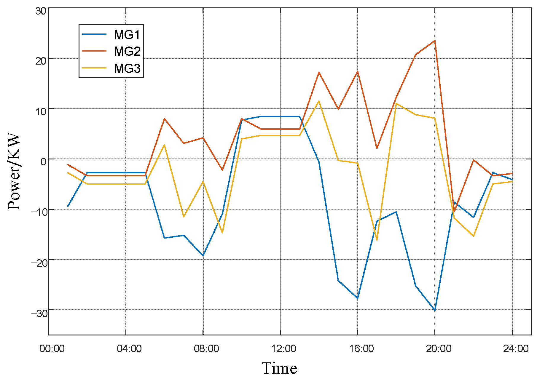
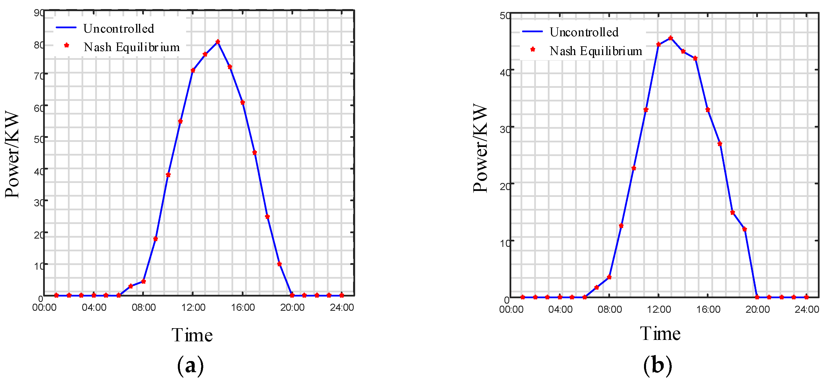
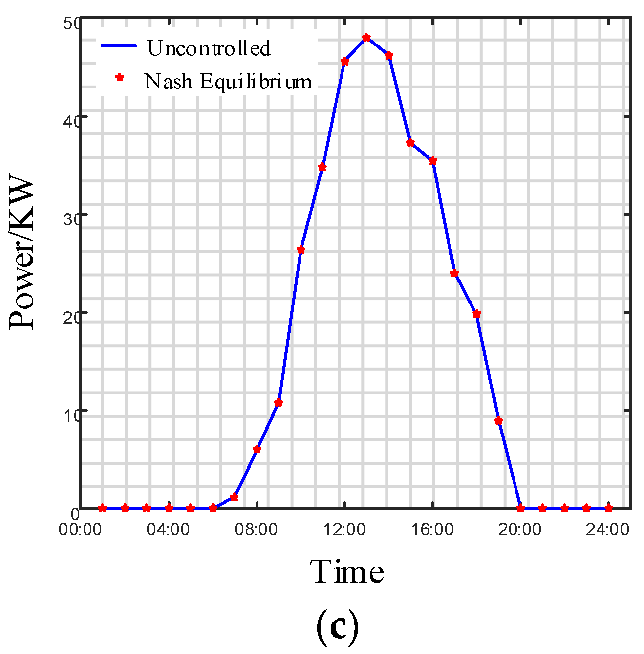
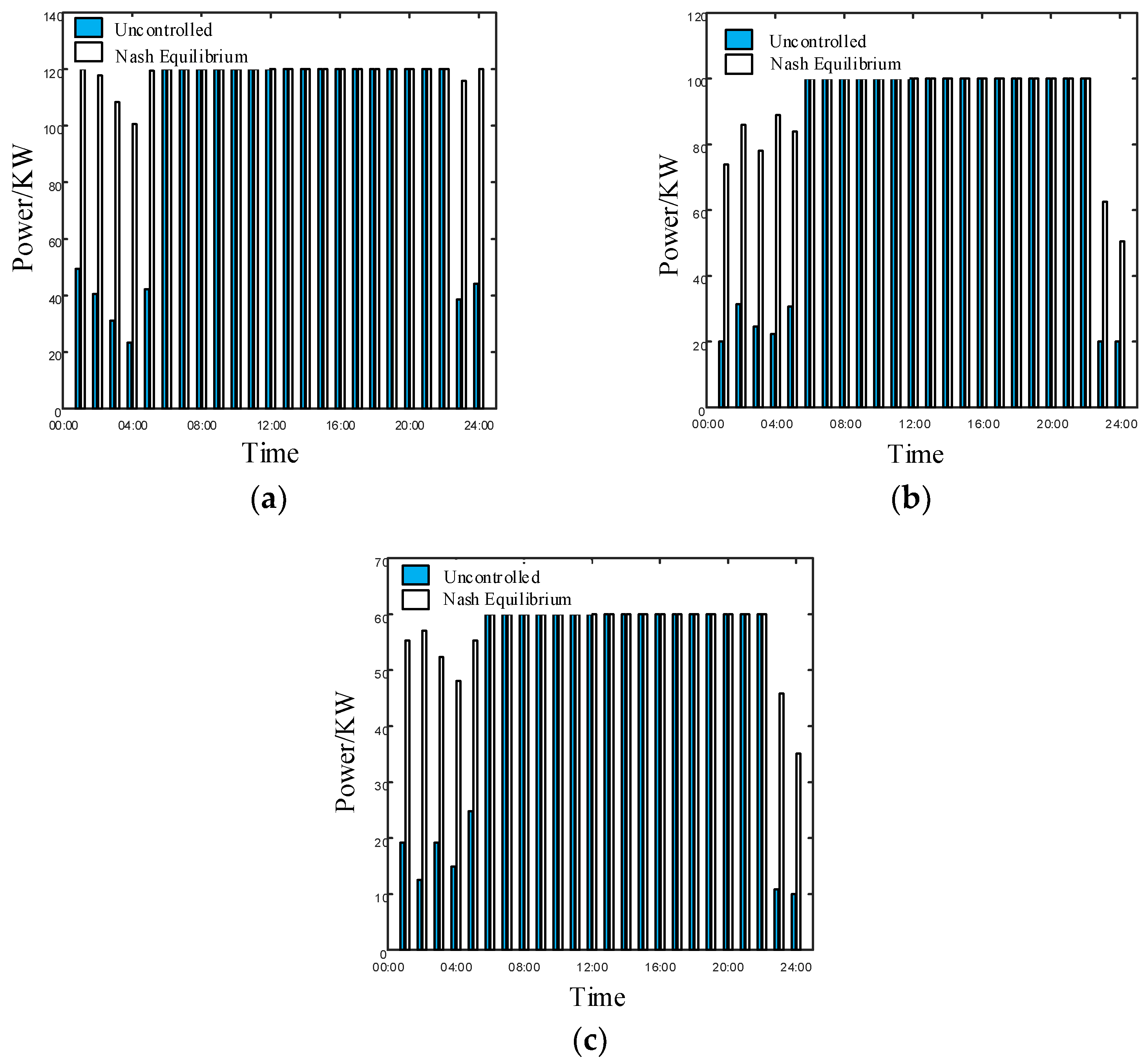
4. Case Studies and Discussion

The historical data of three microgrids in a coastal region of Singapore are employed for a case study. The predicted power curves of PV, WT and load in each microgrid are shown in Figure 5, Figure 6 and Figure 7. The equipment parameters within each microgrid are shown in

Table 3. Microgrid equipment parameters.

Parameter	MG1	MG2	MG3
PFC,max (kW)	120	100	60
PFC,min (kW)	20	20	10
PMT,max (kW)	130	100	65
PMT,min (kW)	20	10	10
PV generation capacity (kW)	100	60	60
Wind turbine generation capacity (kW)	100	60	60
Pbat,ac,max (kW)	20	20	20
Pbat,dc,max (kW)	20	20	20
Energy storage system capacity (kW)	100	100	100
ηbat,ac	0.95	0.95	0.95
ηbat,dc	0.95	0.95	0.95
cbat,ac (CNY/kWh)	0.15	0.15	0.15
cbat,dc (CNY/kWh)	0.15	0.15	0.15

. The base electricity price of the grid is shown in

Table 4. Base electricity price for each time period of the grid.

Time Period	Electricity Price (CNY/kWh)	Time Period	Electricity Price (CNY/kWh)
1	0.32	13	0.95
2	0.32	14	0.95
3	0.32	15	0.63
4	0.32	16	0.63
5	0.32	17	0.63
6	0.63	18	0.95
7	0.63	19	0.95
8	0.63	20	0.95
9	0.63	21	0.63
10	0.95	22	0.63
11	0.95	23	0.32
12	0.95	24	0.32

. The price multiplier b(t) is taken as 0.005. Based on MATLAB software programming, the simulation is solved for optimal operation of an AC/DC microgrid cluster.

The power transaction curve and transaction electricity price of each microgrid under Nash equilibrium are shown in Figure 8 and Figure 9, respectively.

The power transaction curve and transaction electricity price of each microgrid under Nash equilibrium are shown in Figure 8 and Figure 9, respectively. Figure 8 and Figure 9 are concretely analyzed as follows.

(1) During 00:00–5:00 and 23:00–24:00, the grid transaction electricity price is a minimum of 0.32 CNY/kWh, and all three microgrids purchase power. As the total amount of power purchased by the three microgrids increases, the transaction electricity price also increases. The three microgrids stop purchasing power when the transaction electricity price rises to 0.37 CNY/kWh. The remaining energy demand is supplied by fuel cells. The batteries are charged during this period.

(2) During 6:00–9:00, 15:00–17:00 and 21:00–22:00, the fuel cell is operating at full load. MG1 and MG3 purchase electricity and MG2 sells electricity. MG1 purchases a maximum of 27.1 kW at 16:00, MG3 purchases a maximum of 16.1 kW at 17:00, and MG2 sells a maximum of 17.4 kW at 16:00. The overall power transaction state between the three microgrids and the large power grid (or the electric market) is purchasing power. MG1 and MG3 stop purchasing power when the transaction electricity price reaches 0.74 CNY/kWh. The shortage of electricity is provided for by micro gas turbines.

(3) During 10:00–14:00, when the maximum external electricity price is 0.95 CNY/kWh, all three microgrids are in the selling state. The batteries are discharged, and the FCs and MTs are initially operating at full load. When the transaction electricity price drops to 0.86 CNY/kWh, the MT stops generating electricity.

(4) During 18:00–20:00, MG1 is in power purchase state due to its own load, while MG2 and MG3 are still selling power. The overall transaction power of the three microgrids is in the state of selling power. The transaction electricity price decreases from 0.95 CNY/kWh to 0.926 CNY/kWh.

The power transaction curve in Figure 8 shows that each microgrid can both purchase and sell electricity. Figure 9 shows that the transaction electricity price increases with the overall purchase power increasing while the price decreases with the decrease in the total power in the microgrid cluster.

The payment cost of each microgrid is shown in Figure 10. The total payment cost of the microgrid cluster is 6225.6 CNY without coordinated operation of the microgrid cluster (named as uncontrolled operation), and the overall payment cost in Nash equilibrium decreases to 4743.6 CNY, which is 23.8% lower. In summary, the Nash equilibrium state enables power coordination among microgrids and reduces the payment cost. Each microgrid maximizes its own benefits in the Nash equilibrium state.

Based on Equation (39), the total payment cost of the microgrid cluster at maximum economic benefit solution is 4710.6 CNY, and the Pos calculated from Equation (41) is 1.007. The overall benefit in Nash equilibrium is reduced by 0.7% compared with the maximum economic benefits. It can be seen that the Nash equilibrium state has high efficiency and the benefit loss of each microgrid due to competition is small compared with uncontrolled operation of the microgrid cluster.

In fact, the price multiplier b(t) has a large impact on the operation strategies of each microgrid. The value of the price multiplier generally depends on the fluctuation range of the grid 24-h electricity price and the microgrid power limit. The corresponding Pos values for different price multipliers are given in

Table 5. Correspondence between price multiplier and Pos.

Price Multiplier	Pos	Price Multiplier	Pos
0.001	1.0015	0.006	1.0075
0.002	1.0028	0.007	1.0083
0.003	1.0047	0.008	1.0089
0.004	1.0062	0.009	1.0093
0.005	1.007	0.01	1.0097

. It can be seen that as the price multiplier increases, Pos also increases, i.e., the efficiency under Nash equilibrium decreases with the increase in the price multiplier.

From Figure 11, Figure 12, Figure 13 and Figure 14, the output power comparisons of PV, WT, MT, and FC operating under uncontrolled operation and Nash equilibrium state, respectively, are shown.

As can be seen from Figure 11 and Figure 12, the output power of PV and WT is not regulated under Nash equilibrium state. This is because PV and WT have low environmental pollution, zero consumption fuel, and low maintenance costs; thus, they operate at maximum power.

From Figure 13, it can be seen that Nash equilibrium has significant regulating effects on FCs and MTs. Compared with uncontrolled operation, the output power of FCs is greater significantly under Nash equilibrium during 0:00–5:00 and 23:00–24:00, while the output power of FC is not regulated during 6:00–22:00. This is because, compared to the MT, the FC has relatively low pollution cost and thus has priority to generate electricity. During 6:00–22:00, the FCs operate at maximum power. During this period, the insufficient energy is provided by MT, ESS and electricity transaction when the load is high. During 0:00–5:00 and 23:00–24:00, the output power of FCs is still high because the excess energy is charged to ESS. Compared with purchasing electricity in high-load hours, charging the batteries by FCs during 0:00–5:00 and 23:00–24:00 is, overall, cheaper because the energy storage can be used in high-load hours with a high electricity price.

From Figure 14, it can be seen that Nash equilibrium also has significant regulating effects on MTs. Compared with uncontrolled operation, the output power of MTs is generally lower under Nash equilibrium in MG2 and MG3 while the output power of MTs in MG1 is higher under Nash equilibrium. In MG2 and MG3, less electricity from MTs is used due to high output power of FCs in low-load hours. However, the output power of MTs in MG3 is generally higher than that in MG2 because the FCs in MG3 operate at maximum power of 60 kW while the maximum power of FCs in MG2 is 100 kW. As for MG1, the load is much higher than two other microgrids. Compared with uncontrolled operation, the output power of MTs is generally greater from 6:00–9:00, 15:00–17:00 and 21:00–22:00 to store more energy. Therefore, MG1 can purchase less electricity from 18:00–20:00 and even sell electricity from 10:00–14:00 with a relatively high electricity price for benefits.

5. Conclusions

This paper summarizes the structure and control methods of AC/DC hybrid microgrids, and establishes the mathematical model of each distributed power supply and optimization model of the economic cost, and further establishes the optimization objective function for the economic operation of the AC/DC microgrid.

According to the supply and demand theory, the dynamic adjustment mechanism of electricity price is introduced into microgrid clusters. Based on the game theory, a game model for the optimal operation of N microgrids is established. The non-cooperative game model is proven to be a strict potential game, and the existence and convergence of the Nash equilibrium solution are then proved.

Compared with similar studies, the multi-variable and multi-objective optimization process is transformed into a process of finding the extreme value of the potential function, which greatly simplifies the optimal operation control of AC-DC microgrid clusters. The Nash equilibrium solution is obtained by iterative search algorithm, and the operation strategy of microgrid clusters is obtained. This paper also introduces a new unit of interlinking bidirectional AC/DC converter in the modeling of microgrid. A new multiple objective optimization function has been introduced which incorporates fuel cost, environmental cost, equipment maintenance cost, the transaction cost, and the equivalent cost of power loss in the interlinking converters.

Finally, it is verified that power coordination among microgrids can be realized in the Nash equilibrium state with practical examples. The loss of benefits due to competition from multiple microgrids costs are reduced to 0.7%. Each microgrid maximizes its own interests and the system has a higher overall income.

References

1. Kakigano, H.; Miura, Y.; Ise, T.; Uchida, R. DC micro-grid for super high quality distribution—System configuration and control of distributed generations and energy storage devices. In Proceedings of the 2006 37th IEEE Power Electronics Specialists Conference, Jeju, Korea, 18–22 June 2006; pp. 1–7. [Google Scholar]
2. Ram, R.; Rao, M.V.G. Operation and Control of Grid Connected Hybrid AC/DC Microgrid using Various RES. Int. J. Appl. Eng. Res. 2014, 5, 195–202. [Google Scholar]
3. Khezri, R.; Mahmoudi, A. Review on the state-of-the-art multi-objective optimisation of hybrid standalone/grid-connected energy systems. IET Gener. Transm. Distrib. 2020, 14, 4285–4300. [Google Scholar] [CrossRef]
4. Gregoratti, D.; Matamoros, J. Distributed Energy Trading: The Multiple-Microgrid Case. IEEE Trans. Ind. Electron. 2015, 62, 2551–2559. [Google Scholar] [CrossRef] [Green Version]
5. Lee, J.; Guo, J.; Choi, J.K.; Zukerman, M. Distributed Energy Trading in Microgrids: A Game-Theoretic Model and Its Equilibrium Analysis. IEEE Trans. Ind. Electron. 2015, 62, 3524–3533. [Google Scholar] [CrossRef]
6. Bui, V.H.; Hussain, A.; Im, Y.H.; Kim, H.M. An internal trading strategy for optimal energy management of combined cooling, heat and power in building microgrids. Appl. Energy 2019, 239, 536–548. [Google Scholar] [CrossRef]
7. Zhang, B.; Li, Q.; Wang, L.; Feng, W. Robust optimization for energy transactions in multi-microgrids under uncertainty. Appl. Energy 2018, 217, 346–360. [Google Scholar] [CrossRef]
8. Liu, Y.; Guo, L.; Wang, C. A robust operation-based scheduling optimization for smart distribution networks with multi-microgrids. Appl. Energy 2018, 228, 130–140. [Google Scholar] [CrossRef]
9. Wei, C.; Fadlullah, Z.M.; Kato, N.; Takeuchi, A. GT-CFS: A Game Theoretic Coalition Formulation Strategy for Reducing Power Loss in Micro Grids. IEEE Trans. Parallel Distrib. Systs. 2014, 25, 2307–2317. [Google Scholar] [CrossRef]
10. Dashti, Z.A.; Lotfi, M.M.; Mazidi, M. A Non-Cooperative Game Theoretic Model for Energy Pricing in Smart Distribution Networks Including Multiple Microgrids. In Proceedings of the 2019 27th Iranian Conference on Electrical Engineering (ICEE), Yazd, Iran, 30 April–2 May 2019; pp. 808–812. [Google Scholar]
11. Dong, X.; Li, X.; Cheng, S. Energy Management Optimization of Microgrid Cluster Based on Multi-Agent-System and Hierarchical Stackelberg Game Theory. IEEE Access 2020, 8, 206183–206197. [Google Scholar] [CrossRef]
12. Mondal, A.; Misra, S.; Obaidat, M.S. Distributed Home Energy Management System with Storage in Smart Grid Using Game Theory. IEEE Syst. J. 2017, 11, 1857–1866. [Google Scholar] [CrossRef]
13. Park, S.; Lee, J.; Bae, S.; Hwang, G.; Choi, J.K. Contribution-Based Energy-Trading Mechanism in Microgrids for Future Smart Grid: A Game Theoretic Approach. IEEE Trans. Ind. Electron. 2016, 63, 4255–4265. [Google Scholar] [CrossRef]
14. Park, S.; Lee, J.; Hwang, G.; Choi, J.K. Event-Driven Energy Trading System in Microgrids: Aperiodic Market Model Analysis with a Game Theoretic Approach. IEEE Access 2017, 5, 26291–26302. [Google Scholar] [CrossRef]
15. Belgana, A.; Rimal, B.P.; Maier, M. Multi-objective pricing game among interconnected smart microgrids. In Proceedings of the 2014 IEEE PES General Meeting|Conference & Exposition, National Harbor, MD, USA, 27–31 July 2014; pp. 1–5. [Google Scholar]
16. Fu, Y.; Zhang, Z.; Li, Z.; Mi, Y. Energy Management for Hybrid AC/DC Distribution System with Microgrid Clusters Using Non-Cooperative Game Theory and Robust Optimization. IEEE Trans. Smart Grid 2019, 11, 1510–1525. [Google Scholar] [CrossRef]
17. Chen, L.; Niu, Y.; Jia, T. Distributed Energy Seheduling of Islanded Microgrid Based on Potential Game. In Proceedings of the 2020 Chinese Automation Congress (CAC), Shanghai, China, 6–8 November 2020; pp. 1151–1156. [Google Scholar]
18. Wang, W.; Chen, K.; Bai, Y.; Chen, Y.; Wang, J. New estimation method of wind power density with three-parameter Weibull distribution: A case on Central Inner Mongolia suburbs. Wind Energy 2021, 25, 368–386. [Google Scholar] [CrossRef]
19. Zhang, Y.; Jiang, J. Research on Maximum Power Point Tracking Method for Grid-Connected Photovoltaic Power Generation System. In Proceedings of the 2015 International Conference on Automation, Mechanical Control and Computational Engineering, Jinan, China, 24–26 April 2015; pp. 1905–1910. [Google Scholar]
20. Liu, X.; Liu, Y. On the Determination of the Output Power in Mono/Multicrystalline Photovoltaic Cells. Int. J. Photoenergy 2021, 2021, 6692598. [Google Scholar] [CrossRef]
21. Barhoumi, E.M.; Farhani, S.; Bacha, F. High efficiency power electronic converter for fuel cell system application. Ain Shams Eng. J. 2021, 12, 2655–2664. [Google Scholar] [CrossRef]
22. Xu, J.; Zhu, F.; Wang, S. Comprehensive Comparison of Ultra-low Emission Coal-Fired Power Plants and Gas-Fired Power Plants. Electr. Power 2020, 53, 164–172, 179. [Google Scholar]
Figure 1. The structure of typical ac/dc microgrid.
Energies 15 05537 g001
Figure 2. Typical efficiency curve of the converter.
Energies 15 05537 g002
Figure 3. Optimal operation process of microgrid clusters based on game theory.
Energies 15 05537 g003
Figure 4. The solving process of the game model of the AC/DC hybrid microgrid clusters.
Energies 15 05537 g004
Figure 5. WT, PV and load history curve in MG1.
Energies 15 05537 g005
Figure 6. WT, PV and load history curve in MG2.
Energies 15 05537 g006
Figure 7. WT, PV and load history curve in MG3.
Energies 15 05537 g007
Figure 8. Power transaction curve under Nash equilibrium.
Energies 15 05537 g008
Figure 9. Transaction electricity price under Nash equilibrium.
Energies 15 05537 g009
Figure 10. Payment costs for each microgrid.
Energies 15 05537 g010
Figure 11. PV output power curve. (a) PV output power curve in MG1. (b) PV output power curve in MG2. (c) PV output power curve in MG3.
Energies 15 05537 g011aEnergies 15 05537 g011b
Figure 12. WT output power curve. (a) WT output power curve in MG1. (b) WT output power curve in MG2. (c) WT output power curve in MG3.
Energies 15 05537 g012
Figure 13. FC output power. (a) FC output power in MG1. (b) FC output power in MG2. (c) FC output power in MG3.
Energies 15 05537 g013
Figure 14. MT output power. (a) MT output power in MG1. (b) MT output power in MG2. (c) MT output power in MG3.
Energies 15 05537 g014