Robust Multi-Objective H₂/H_∞ Load Frequency Control of Multi-Area Interconnected Power Systems Using TS Fuzzy Modeling by Considering Delay and Uncertainty

Abstract

The main objective of this paper is to design a robust multi-objective ${\mathrm{H}}_2/{\mathrm{H}}_{\infty }$ delayed feedback controller for load frequency control of a multi-area interconnected power system by taking into account all theoretical and practical constraints. To achieve more precise modelling and analysis, the limitation of valve position, governor, and transmission delay are considered to guarantee of LFC system’s stability in practical applications. The nonlinear delayed system is approximated by the Takagi–Sugeno fuzzy model. Then, a parallel distributed compensation scheme is utilized for designing the control system of the overall system. The proposed multi-objective and robust ${\mathrm{H}}_2/{\mathrm{H}}_{\infty }$ controller simultaneously minimizes the ${\mathrm{H}}_2$ and ${\mathrm{H}}_{\infty }$ control performance indexes. Finally, simulation results verify the robustness and effectiveness of the proposed scheme in dealing with the impact of load disturbances, model uncertainties, transmission time delays, and nonlinearities in the model.

1. Introduction

Designing an LFC system is a challenging task in the stable and safe operation of a power system, particularly an interconnected and multi-area power system. Frequency and voltage oscillations typically cause some negative effects on power systems and consumers. Deviation of the auxiliary power machines and generator sets from operational circumstances, reducing the mechanical performance, and affecting the overall economic operation of the power grid are some negative results of this issue [1]. The objective of an LFC system is to damp the frequency and voltage fluctuations in an interconnected power system generated from changes in the connected load instant shifts. During the past few decades, the LFC system design has been studied in many works, by utilizing different control strategies, such as PI controller [2,3,4,5], fuzzy logic [6,7], neural network [8], adaptive control [9], and variable structure control [10].

Moreover, it might be challenging to determine the exact values of some design model parameters. Furthermore, unpredictable changes in load demand are a normal issue in power systems. These problems will unavoidably have an impact on the stable and secure operation of the power systems. Therefore, an LFC system should be robust against parametric uncertainties and load disturbances. In [11], a robust decentralized LFC system was suggested for interconnected power systems to regulate the area control error during uncertainties. In [12], a robust controller based on the FO PID was presented for frequency control of an interconnected power system, and the optimal controller parameters were obtained through differential evolution algorithms. In [13], coordination of conventional frequency and V2G controllers was designed for a robust LFC scheme for a wind farm-based smart grid. In [14], a distributed robust model predictive controller was presented based on LMIs for the LFC system design issues of a multi-area interconnected power system.

Furthermore, delays raised by communication links among various control areas in s multi-area power system should be considered to avoid maloperation and instability of the LFC system. There are only a few solutions in the literature that considered the communication delay during the design of LFC systems. In [15], a decentralized delay-independent and memory-less control strategy were proposed to design a load frequency control system that considered communication delays. In [16], by considering the communication delays, a ${\mathrm{H}}_{\infty }$ two-term delay-dependent feedback control structure was designed for the LFC system of a power system with a multi-area network. However, the uncertainties of the power system were not considered in this research. In [17], a robust ${\mathrm{H}}_{\infty }$ delayed state feedback controller was presented for the LFC of interconnected power systems which have parametric uncertainties and stochastic disturbances.

In practical situations, ${\mathrm{H}}_{\infty }$ synthesis is unable to fully satisfy all design requirements. For example, using linear–quadratic regulator terminology allows for a more natural expression of noise reduction or regulating against unpredictable disturbances. In addition to this, in most cases, a well-designed controller should operate within the lowest operation time, with a well-damped response in addition to the rejection of disturbances on chosen system outputs. Such options make multi-objective synthesis a suitable choice in practical applications. In [18], a mixed ${\mathrm{H}}_2/{\mathrm{H}}_{\infty }$ output feedback control structure using the pole-placement technique was proposed for multi-area load frequency control, but transmission delays and parameter uncertainties are not considered in the model of the system.

Furthermore, in the aforementioned works [16,17,18], typically, a linear model is considered to express the dynamics of the power systems. However, there are some nonlinear characteristics like valve position limits in the power systems which it is necessary to consider in the modeling procedure. A control technique based on the TS fuzzy-model is a very popular method for controlling complex systems with nonlinearity. In [19], a robust controller was developed for the LFC of nonlinear power systems with uncertainty using TS fuzzy modeling. However, the transmission delay was not considered in the design procedure. Moreover, a high gain controller was obtained in [19] which is not reasonable in the implementation phase.

In recent LFC studies, the LFC design of photovoltaic and thermal generators connected by AC tie-line is considered as an early attempt to develop frequency stabilization techniques using I, ID, IDD, PI, and PID determined through the JAYA optimization procedure [20]. In [21], in order to fit tie power exchange and frequency deviation and to the desired values after an unexpected load disturbance in an interconnected system, a collaborative scheme using linear quadratic regulator design and hybrid bacteria foraging-oriented PSO is presented to develop an automatic generation control for power delivery systems by having the power generations from hydro turbines in interconnected control areas. A new control method relying on the FO Type-2 Fuzzy logic system suggested in [22] through PSO to solve the frequency control problem of renewable interconnected power systems in order to restore the power systems to their starting position when a load change occurs. The authors of [23] present a control framework for the LFC of an interconnected hydro–hydro system by a combination of fuzzy logic and a PID controller that is efficiently optimized by PSO. In [24], an active fault-tolerant control technique without parameters of the system is suggested for LFC system design. First, to stable any feasible working scenario, a set of controllers is designed. Then, in order to choose the controller that best fits the system, a zero trial-and-error selection procedure, independent of previous system parameters, is developed. In addition, an expanding technique with no previous faulty information is suggested to improve the fault-tolerant capability in the situation of unmodeled faulty scenarios. In [25], it is addressed how to create an asynchronous FD observer for 2-D MJSs defined by a Roesser model. The FD observer, generally, does not operate synchronously with the system; rather, the observer′s mode changes with the system′s mode in accordance with certain conditional transitional probabilities. For uncovering this challenging issue, a hidden Markov model is used. The FD problem is then solved multi-objectively by integrating the ${\mathrm{H}}_{\infty }$ attenuation index and H increscent index. Furthermore, based on the LMI technique, enough criteria have been established to ensure the asynchronous FD′s occurrence, and to obtain the best performance indices, an asynchronous FD method is simultaneously produced.

Given the above discussion, there still seems to be a deficiency in LFC of multi-area interconnected power systems by taking into account all design limitations including nonlinearities in the system model, functional limitations of all system components, communication time-delays, and uncertainty in system model parameters. On the other hand, it is very important to meet all the control requirements, including the design of a robust controller with practical application to maintaining the system performance with changes in the load demand. To achieve this goal, in addition to the ability to reject the disturbance effect, the designed controller should have an appropriate control gain. In addition to this, achieving a time response with a suitable transient specification is very crucial. The proposed method could be used for thermal, wind, and hydroelectric power plants.

The main novel contributions of this paper are as follows:

• Considering all operational limitations of the investigated power system (transmission time delay, nonlinearity of governor, and load changes) in process of designing an LFC system;
• Considering all robust performances (presence of model parametric uncertainties and external disturbances);

• Designing a robust ${\mathrm{H}}_2/{\mathrm{H}}_{\infty }$ multi-objective controller (${\mathrm{H}}_{\infty }$ performance for rejecting the disturbance and uncertainty effects and ${\mathrm{H}}_2$ performance for improving the transient responses and achieving a reasonable and implementable controller with appropriate gains);

• Utilizing TS fuzzy modelling for linearization of the nonlinear system with proper accuracy.

The rest of the paper is organized as follows. In Section 2, mathematical models for developing an LFC system are presented. The TS fuzzy model of a multi-area power system considering the valve position limits on the governor is developed in Section 3. The robust delayed feedback controller design procedure and PDC scheme are proposed in Section 4. The simulation results are given in Section 5. Finally, the paper is concluded with some conclusions in Section 6.

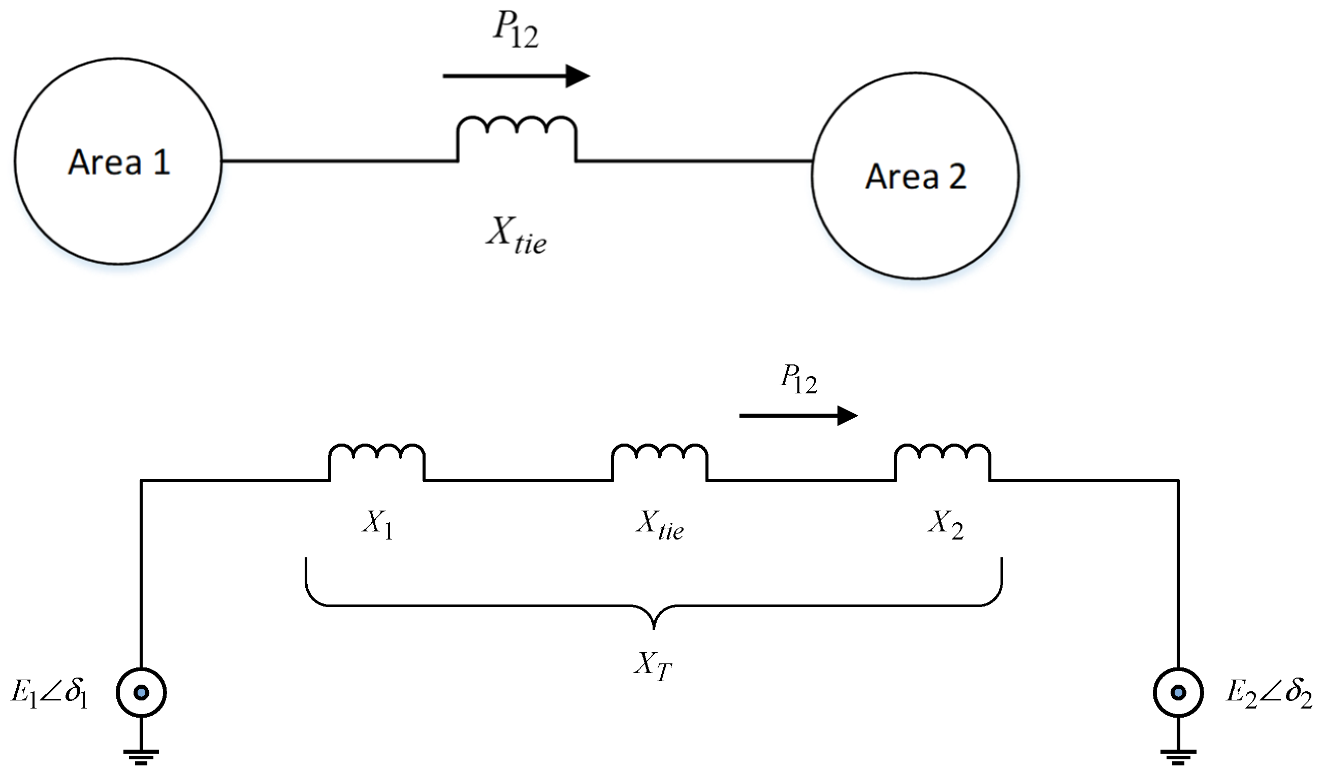
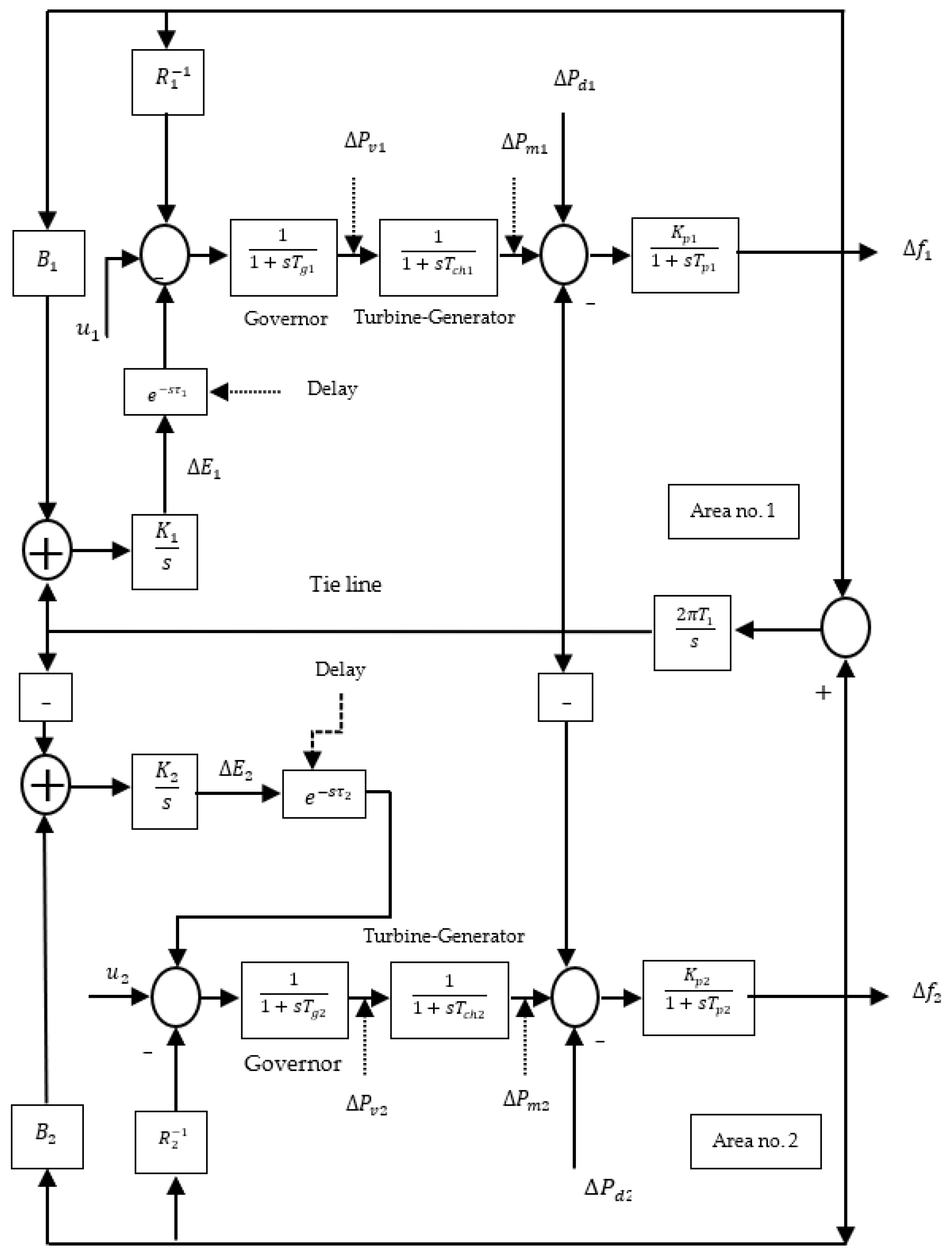
2. LFC Model Description

A simple representation of a two-area system and its electrical equivalent circuit is illustrated in Figure 1.

The overall block diagram of two-area interconnected power systems with communication delays is depicted in Figure 2. In an LFC system, there are always delays in the communication networks among the controller unit and operational units; especially on the measured tie-line power flow and frequency. These time delays have an effect on the system operation and even cause instability in the LFC system. Hence, it is pivotal to consider this issue during the designing process of an LFC system.

It can be seen that there is a local PI controller in both control areas as an integral part of the model. The differential equations of the delayed multi-area power system can be formulated as [16,17]:

$$\begin{array}{l}\Delta {\dot{P}}_{mi}(\mathrm{t})=\frac{\Delta P_{vi}(\mathrm{t})}{T_{chi}}-\frac{\Delta P_{mi}(\mathrm{t})}{T_{chi}}\\ \Delta {\dot{E}}_i(\mathrm{t})=-k_i\Delta P_{12}(\mathrm{t})+k_i{B}_i\Delta f_i(\mathrm{t})\\ \Delta {\dot{P}}_{12}(\mathrm{t})=2\pi {\mathrm{T}}_1\Delta f_1(\mathrm{t})-2\pi {\mathrm{T}}_1\Delta f_2(\mathrm{t})\\ \Delta {\dot{P}}_{vi}(\mathrm{t})=-\frac{\Delta f_i(\mathrm{t})}{R_i{T}_{gi}}-\frac{\Delta P_{vi}(\mathrm{t})}{T_{gi}}-\frac{\Delta E(\mathrm{t}-{\tau }_i)}{T_{gi}}+\frac{u_i(\mathrm{t})}{T_{gi}}\\ \Delta {\dot{f}}_i(\mathrm{t})=-\frac{k_{pi}\Delta P_{di}(\mathrm{t})}{T_{pi}}-\frac{k_{pi}\Delta P_{ij}(\mathrm{t})}{T_{pi}}+\frac{k_{pi}\Delta P_{mi}(\mathrm{t})}{T_{pi}}-\frac{\Delta f_i(\mathrm{t})}{T_{pi}}\end{array}$$

(1)

where

$P_{12}=-P_{21}, i,j=1,2,i\ne j,$ and τ_i is the transmission delay of i^th area that arises in two situations; first, during transmission of the telemetered signals to the local control center by RTUs, and second, when ACE signals transmit from the control unit to the generator unit [16].

In the situation of a large change in load disturbance $\Delta P_{di}$, the linear model (1) cannot be a good approximation of a practical system. This inaccuracy is resulted from the governor valve position limitations due to its mechanical structure [26,27]. This means that when a large $\Delta P_{di}$ occurs, a large change in speed changer position $\Delta P_{ci}$ is required to regulate the frequency deviation $\Delta f_i$; however, the governor output $\Delta P_{vi}$ will not change beyond a specific level. This being the case, it is essential to design an LFC system to guarantee the power system stability with this limitation. A piston-like steam valve system is illustrated in Figure 3 used in this paper to model the valve position limitations. A nonlinear function ${\beta }_i\left(\Delta P_{vi}(\mathrm{t})\right)$ is defined as follows to represent the governor valve position limit.

$${\beta }_i\left(\Delta P_{vi}(\mathrm{t})\right)=\{\begin{array}{cc}\Delta P_{v{i}_{\min }}& \Delta P_{vi}(\mathrm{t})\le \Delta P_{v{i}_{\min }}\\ \Delta P_{vi}& \Delta P_{v{i}_{\min }}\le \Delta P_{vi}(\mathrm{t})\le \Delta P_{v{i}_{\max }}\\ \Delta P_{v{i}_{\max }}& \Delta P_{vi}(\mathrm{t})\ge \Delta P_{v{i}_{\max }}\end{array}$$

(2)

Now, by considering valve position limitations, the nonlinear differential equations of the system are rewritten as follows:

$$\{\begin{array}{l}\Delta {\dot{f}}_1(\mathrm{t})=-\frac{k_{p1}\Delta P_{d1}(\mathrm{t})}{T_{p1}}-\frac{k_{p1}\Delta P_{12}(\mathrm{t})}{T_{p1}}+\frac{k_{p1}\Delta P_{m1}(\mathrm{t})}{T_{p1}}-\frac{\Delta f_1(\mathrm{t})}{T_{p1}}\\ \Delta {\dot{P}}_{m1}(\mathrm{t})=\frac{{\beta }_1\left(\Delta P_{v1}(\mathrm{t})\right)}{T_{ch1}}-\frac{\Delta P_{m1}(\mathrm{t})}{T_{ch1}}\\ \Delta {\dot{P}}_{v1}(\mathrm{t})=-\frac{\Delta f_1(\mathrm{t})}{R_1{T}_{g1}}-\frac{\Delta P_{v1}(\mathrm{t})}{T_{g1}}-\frac{\Delta E_1(\mathrm{t}-{\tau }_1)}{T_{g1}}+\frac{\Delta P_{c1}(\mathrm{t})}{T_{g1}}\\ \Delta {\dot{E}}_1(\mathrm{t})=-k_1\Delta P_{12}(\mathrm{t})+k_1{B}_1\Delta f_1(\mathrm{t})\\ \Delta {\dot{P}}_{12}(\mathrm{t})=2\pi {\mathrm{T}}_1\Delta f_1(\mathrm{t})-2\pi {\mathrm{T}}_1\Delta f_2(\mathrm{t})\\ \Delta {\dot{f}}_2(\mathrm{t})=-\frac{k_{p2}\Delta P_{d2}(\mathrm{t})}{T_{p2}}+\frac{k_{p2}\Delta P_{12}(\mathrm{t})}{T_{p2}}+\frac{k_{p2}\Delta P_{m2}(\mathrm{t})}{T_{p2}}-\frac{\Delta f_2(\mathrm{t})}{T_{p2}}\\ \Delta {\dot{P}}_{m2}(\mathrm{t})=\frac{{\beta }_2\left(\Delta P_{v2}(\mathrm{t})\right)}{T_{ch2}}-\frac{\Delta P_{m2}(\mathrm{t})}{T_{ch2}}\\ \Delta {\dot{P}}_{v2}(\mathrm{t})=-\frac{\Delta f_2(\mathrm{t})}{R_2{T}_{g2}}-\frac{\Delta P_{v2}(\mathrm{t})}{T_{g2}}-\frac{\Delta E_2(\mathrm{t}-{\tau }_2)}{T_{g2}}+\frac{\Delta P_{c2}(\mathrm{t})}{T_{g2}}\\ \Delta {\dot{E}}_2(\mathrm{t})=-k_2\Delta P_{12}(\mathrm{t})+k_2{B}_2\Delta f_2(\mathrm{t})\end{array}$$

(3)

3. TS Fuzzy Modeling

In this section, the design stage begins with describing the nonlinear systems using the TS fuzzy model. This model is represented by the fuzzy IF-THEN rules that comprise local linear input–output relations of the nonlinear system in their consequent parts.

To obtain the system’s TS fuzzy model, membership functions are defined as follows:

$$\begin{array}{l}{M}_1^i\left(\Delta P_{vi}\right)=\frac{{\beta }_i\left(\Delta P_{vi}\right)-{\xi }_i\Delta P_{vi}}{\left(1-{\xi }_i\right)\Delta P_{vi}}\\ M_2^i\left(\Delta P_{vi}\right)=\frac{\Delta P_{vi}-{\beta }_i\left(\Delta P_{vi}\right)}{\left(1-{\xi }_i\right)\Delta P_{vi}}\end{array}$$

(4)

where

$$\begin{array}{l}{\beta }_i\left(\Delta P_{vi}\right)=M_1^i\left(\Delta P_{vi}\right)\Delta P_{vi}+M_2^i\left(\Delta P_{vi}\right){\xi }_i\Delta P_{vi}\\ M_1^i\left(\Delta P_{vi}\right)+M_2^i\left(\Delta P_{vi}\right)=1\\ \begin{array}{cc}{\xi }_i=Min\left(\left|\frac{\Delta P_{v{i}_{\min }}}{Q_i^L}\right|,\left|\frac{\Delta P_{v{i}_{\max }}}{Q_i^U}\right|\right),& \Delta P_{vi}\in \left[Q_i^L,Q_i^U\right]\end{array}\end{array}$$

(5)

Next, the TS fuzzy system is defined by fuzzy IF-THEN rules. The ith rule of the TS fuzzy model is given as follows:

Model Rule i:

If $z_1(\mathrm{t})$ is ${\mathrm{M}}_1^{\mathrm{i}}$ and $z_2(\mathrm{t})$ is ${\mathrm{M}}_2^{\mathrm{i}}$

Then

$$\{\begin{array}{l}\dot{x}(t)=\left(A_i+\Delta A_i\right)x(t)+\left(A_{d_1}+\Delta A_{d_1}\right)x(t-{\tau }_1)+\left(A_{d_2}+\Delta A_{d_2}\right)x(t-{\tau }_2)+Bu(t)+Dw(t)\\ y(t)=Cx(t)\end{array}$$

(6)

where $\mathrm{Z}(\mathrm{t})={\left[z_1(\mathrm{t}),z_2(\mathrm{t})\right]}^T$ is the premise variable vector, $x(\mathrm{t})=\left[\Delta f_1,\Delta P_{m1},\Delta P_{v1},\Delta E_1,\Delta P_{12},\Delta f_2,\Delta P_{m2},\Delta P_{v2},\Delta E_2\right]$ is the state vector, $u(\mathrm{t})={\left[\Delta P_{c1},\Delta P_{c2}\right]}^T$ is the control input vector, $w(\mathrm{t})={\left[\Delta P_{d1},\Delta P_{d2}\right]}^T$ is the disturbance input vector, and $y(\mathrm{t})={\left[\Delta f_1,\Delta f_2\right]}^T$ is the output vector and $A_{d1}$, $A_{d2}$ are the matrices that present the delayed dynamics of the system.

Furthermore, $A_i$, $A_{d1}$, $A_{d2}$, $B$, $C$, and $D$ are known constant matrices as follows:

$$\begin{array}{c}{A}_i=\left[\begin{array}{ccccccccc}-\frac{1}{T_{p1}}& \frac{K_{p1}}{T_{p1}}& 0& 0& -\frac{K_{p1}}{T_{p1}}& 0& 0& 0& 0\\ 0& -\frac{1}{T_{ch1}}& {\left(2,3\right)}_i& 0& 0& 0& 0& 0& 0\\ -\frac{1}{R_1{T}_{g1}}& 0& -\frac{1}{T_{g1}}& 0& 0& 0& 0& 0& 0\\ K_1{B}_1& 0& 0& 0& -K_1& 0& 0& 0& 0\\ 2\pi T_1& 0& 0& 0& 0& -2\pi T_1& 0& 0& 0\\ 0& 0& 0& 0& \frac{K_{p2}}{T_{p2}}& -\frac{1}{T_{p2}}& \frac{K_{p2}}{T_{p2}}& 0& 0\\ 0& 0& 0& 0& 0& 0& -\frac{1}{T_{ch2}}& {\left(7,8\right)}_i& 0\\ 0& 0& 0& 0& 0& -\frac{1}{R_2{T}_{g2}}& 0& -\frac{1}{T_{g2}}& 0\\ 0& 0& 0& 0& -K_2& K_2{B}_2& 0& 0& 0\end{array}\right]\\ \begin{array}{cc}{A}_{d_1}=\left[\begin{array}{ccccccccc}0& 0& 0& 0& 0& 0& 0& 0& 0\\ 0& 0& 0& 0& 0& 0& 0& 0& 0\\ 0& 0& 0& -\frac{1}{T_{g1}}& 0& 0& 0& 0& 0\\ 0& 0& 0& 0& 0& 0& 0& 0& 0\\ 0& 0& 0& 0& 0& 0& 0& 0& 0\\ 0& 0& 0& 0& 0& 0& 0& 0& 0\\ 0& 0& 0& 0& 0& 0& 0& 0& 0\\ 0& 0& 0& 0& 0& 0& 0& 0& 0\\ 0& 0& 0& 0& 0& 0& 0& 0& 0\end{array}\right],& \end{array}{A}_{d_2}=\left[\begin{array}{ccccccccc}0& 0& 0& 0& 0& 0& 0& 0& 0\\ 0& 0& 0& 0& 0& 0& 0& 0& 0\\ 0& 0& 0& 0& 0& 0& 0& 0& 0\\ 0& 0& 0& 0& 0& 0& 0& 0& 0\\ 0& 0& 0& 0& 0& 0& 0& 0& 0\\ 0& 0& 0& 0& 0& 0& 0& 0& 0\\ 0& 0& 0& 0& 0& 0& 0& 0& 0\\ 0& 0& 0& 0& 0& 0& 0& 0& -\frac{1}{T_{g2}}\\ 0& 0& 0& 0& 0& 0& 0& 0& 0\end{array}\right]\\ \begin{array}{cc}\begin{array}{cc}B=\left[\begin{array}{cc}0& 0\\ 0& 0\\ \frac{1}{T_{g1}}& 0\\ 0& 0\\ 0& 0\\ 0& 0\\ 0& 0\\ 0& \frac{1}{T_{g2}}\\ 0& 0\end{array}\right],& \end{array}& C=\left[\begin{array}{ccccccccc}1& 0& 0& 0& 0& 0& 0& 0& 0\\ 0& 0& 0& 0& 0& 1& 0& 0& 0\end{array}\right]\end{array}, D=\left[\begin{array}{cc}-\frac{K_{p1}}{T_{p1}}& 0\\ 0& 0\\ 0& 0\\ 0& 0\\ 0& 0\\ 0& -\frac{K_{p2}}{T_{p2}}\\ 0& 0\\ 0& 0\\ 0& 0\end{array}\right]\end{array}$$

where

$$\begin{gathered} {\left(2,3\right)}_1={\left(2,3\right)}_3=\frac{1}{T_{c{h}_1}}, {\left(2,3\right)}_2={\left(2,3\right)}_4=\frac{{\xi }_1}{T_{c{h}_1}} \\ {\left(7,8\right)}_1={\left(7,8\right)}_2=\frac{1}{T_{c{h}_2}}, {\left(7,8\right)}_3={\left(7,8\right)}_4=\frac{{\xi }_2}{T_{c{h}_2}} \end{gathered}$$

Furthermore, $\Delta A_i$, $\Delta A_{d1}$, and $\Delta A_{d2}$ denote the parametric uncertainties. Without losing generality, these uncertainties of parameters are typically considered to fulfill.

$$\left[\Delta A_i,\Delta A_{d_1},\Delta A_{d_2}\right]=MF(\mathrm{t})\left[N_1,N_2,N_3\right]$$

(7)

where $N_1$, $N_2$, $N_3$, and $M$ are the known constant matrices with proper dimensions, and the nonlinear uncertain matrix $F(\mathrm{t})$ fulfills.

$$F^T(t)F(t)\le I$$

(8)

Thus, the overall uncertain delayed T-S fuzzy system is represented as:

$$\begin{array}{l}\dot{x}(t)={\displaystyle \sum _{i=1}^q{h}_i\left(z(\mathrm{t})\right)\left(\left(A_i+\Delta A_i\right)x(t)+\left(A_{d_1}+\Delta A_{d_1}\right)x(t-{\tau }_1)+\left(A_{d_2}+\Delta A_{d_2}\right)x(t-{\tau }_2)+Bu(t)+Dw(t)\right)}\\ y(t)={\displaystyle \sum _{i=1}^q{h}_i\left(z(\mathrm{t})\right)Cx(t)}\end{array}$$

(9)

where $h_i\left(z(t)\right)$ is the normalized membership function corresponds to $i^{th}$ the rule and is defined as follows:

$$h_i\left(z(t)\right)=\frac{{\alpha }_i\left(z(\mathrm{t})\right)}{{\displaystyle \sum _{i=1}^q{\alpha }_i\left(z(\mathrm{t})\right)}}$$

(10)

where ${\alpha }_i\left(z(\mathrm{t})\right)=M_1^i\left(z_1(\mathrm{t})\right)\times M_2^i\left(z_2(\mathrm{t})\right)$.

4. Proposed Robust $H_2/H_{\infty }$ Control Based on the PDC Scheme

${\mathrm{H}}_{\infty }$ control is one of the most efficient controllers to attenuate the effects of external disturbances and parametric uncertainties. However, these control structures typically cause large gains and greatly magnify noises, degrading efficiency. In this situation, the combination of ${\mathrm{H}}_2$ and ${\mathrm{H}}_{\infty }$ controllers can be effective to keep the control signal within practical bounds, because it considers a trade-off between the robustness and the control cost. Moreover, the ${\mathrm{H}}_2$ controller improves closed-loop system time responses including settling time, overshoot, and a maximum frequency of response.

By assuming the following delayed LFC system with parametric uncertainties:

$$\{\begin{array}{l}\dot{x}(t)=\left(A+\Delta A\right)x(t)+\left(A_{d_1}+\Delta A_{d_1}\right)x(t-{\tau }_1)+\left(A_{d_2}+\Delta A_{d_2}\right)x(t-{\tau }_2)+Bu(t)+Dw(t)\\ y(t)=Cx(t)\end{array}$$

(11)

A delay-dependent state feedback controller is proposed as follows:

$$u(t)=Kx(t)+K_{d}x(t-\tau )$$

(12)

The resulting LFC system could be as follows:

$$\{\begin{array}{l}\dot{x}(t)=\left(A+\Delta A+BKC\right)x(t)+\left(A_{d_1}+\Delta A_{d_1}\right)x(t-{\tau }_1)+\left(A_{d_2}+\Delta A_{d_2}\right)x(t-{\tau }_2)+Dw(t)+B{K}_{d}x(t-\tau )\\ y(t)=Cx(t)\end{array}$$

(13)

The relationship between the interference and output can be represented as $T_{wy}(s)=C{\left[SI-\left(A+\Delta A+BKC\right)-\left(A_1+\Delta A_1\right)e^{-{\tau }_{1}s}-\left(A_2+\Delta A_2\right)e^{-{\tau }_{2}s}+B{K}_d{e}^{-\tau s}\right]}^{-1}D$.

4.1. $H_{\infty }$ Controller Design

Let $T_{wy}$ as closed-loop transfer function from the disturbance vector $w(t)$ to the output vector $y(t)$. The aim is to develop the state feedback controller (12) such that satisfy the following inequality:

$$\Vert T_{wy}\Vert \le \gamma$$

(14)

where $\gamma$ is ${\mathrm{H}}_{\infty }$ performance index showing the measured disturbance rejection of the robust controller. It is clear that a smaller value of $\gamma$ indicates better robustness performance.

Theorem 1 [17].

The delayed uncertain close-loop LFC system (13) with the control law (12) meets the $H_{\infty }$performance index (14), if there exist a scalar $\epsilon >0$, matrices $X=X^T>0$, $H_1=H_1^T>0$, $H_2=H_2^T>0$, $H_3=H_3^T>0$, $Z_a=Z_a^T>0$ and, $S$, $V$, $E_a$, $F_a$ such that the following LMI holds.

$$\Sigma =\left[\begin{array}{ccccccccc}{\Sigma }_{11}& {\Sigma }_{12}& A_{1}X& A_{2}X& {\Sigma }_{15}& \tau E_a& D& X{C}^T& XM\\ *& {\Sigma }_{22}& 0& 0& V^T{B}^T& \tau F_a& 0& 0& 0\\ *& *& {\Sigma }_{33}& 0& X{A}_1^T& 0& 0& 0& 0\\ *& *& *& {\Sigma }_{44}& X{A}_2^T& 0& 0& 0& 0\\ *& *& *& *& {\Sigma }_{55}& 0& D& 0& XM\\ *& *& *& *& *& -\tau Z_a& 0& 0& 0\\ *& *& *& *& *& *& -I& 0& 0\\ *& *& *& *& *& *& *& -{\gamma }^{2}I& 0\\ *& *& *& *& *& *& *& *& -\epsilon I\end{array}\right]<0$$

(15)

where

$$\begin{array}{c}X=G^{-1},H_i=G^{-1}{Q}_i{G}^{-1}\left(i=1,2,3\right),E_a=G^{-1}E{G}^{-1},\hfill \\ F_a=G^{-1}F{G}^{-1},Z_a=G^{-1}Z{G}^{-1},\hfill \\ {\Sigma }_{11}=\left(AX+BS\right)+{\left(AX+BS\right)}^T\underset{x\to \infty }{\lim }+H_1+H_2+H_3+E_a+E_a^T+\epsilon N_1^T{N}_1,\hfill \\ P_a=G^{-1}P{G}^{-1},{\Sigma }_{12}=BV-E_a+F_a^T,{\Sigma }_{15}=-X+{\left(AX+BS\right)}^T+P_a,\hfill \\ {\Sigma }_{33}=-H_1+\epsilon N_2^T{N}_2, {\Sigma }_{22}=-H_3-F_a-F_a^T,{\Sigma }_{55}=\tau Z_a-X-X^T,\hfill \\ {\Sigma }_{44}=-H_3+\epsilon N_3^T{N}_3,\hfill \end{array}$$

The optimized attenuation level $\gamma$ could be determined by the following subject and (14):

$$\begin{array}{c}\mathrm{Min} {\delta }_0={\gamma }^2\\ \mathrm{Subject} \mathrm{to} X>0,H_1>0,H_2>0,H_3>0,Z_a>0,S,V,{\mathrm{E}}_a,F_a\end{array}$$

(16)

4.2. $H_2$ Controller Design

Consider the time delay (11) in an uncertain LFC system. If a positive scalar $J^{*}$ and a control rule $u^{*}(\mathrm{t})$ exist for all permissible uncertainties, the closed-loop system will be stable, and the cost function’s closed-loop value is defined as follows:

$$J={\displaystyle {\int }_0^{\infty }\left[X^T(t)Q(t)+u^T(t)Ru(t)\right]}dt$$

(17)

By satisfying $J\le J^{*}$, then $J^{*}$ is guaranteed cost and $u^{*}(\mathrm{t})$ is guaranteed cost control law of the system. Where R and Q are positive-definite symmetric matrices [28] that determine the weight of state variables and control variables in the cost function (17), respectively. Since the importance of state and input variables is the same in this research, both matrices are considered identity matrices.

Theorem 2 [28].

Assume the delayed LFC system with parametric uncertainties (11) with cost function (17). If the optimization problem (18–21) has a solution$\epsilon ,\alpha ,\mathrm{W},\mathrm{X},\mathrm{V},\mathrm{T}$, then the control rule$u(t)=W{X}^{-1}x(t)$is the optimal state feedback guaranteed cost control rule that guarantees the optimization of the guaranteed cost (17) for the time-delay system with parametric uncertainties.

$$\mathrm{Min} {}_{\epsilon ,\alpha ,W,V,T }\alpha +tr(T)$$

(18)

Subject to

$$\left[\begin{array}{cccccc}\tilde{A}& A_{d_1}V& {\left(N_{1}X+N_{2}W\right)}^T& X& W^T& X\\ V{A}_{d_1}^T& -V& V{N}_3^T& 0& 0& 0\\ N_{1}X+N_{2}W& N_{3}V& -\epsilon I& 0& 0& 0\\ X& 0& 0& -Q^{-1}& 0& 0\\ W& 0& 0& 0& -R^{-1}& 0\\ X& 0& 0& 0& 0& -V\end{array}\right]<0$$

(19)

$$\left[\begin{array}{cc}-\alpha & {\phi }^T\left(0\right)\\ \phi \left(0\right)& -X\end{array}\right]<0$$

(20)

$$\left[\begin{array}{cc}-T& N^T\\ N& -V\end{array}\right]<0$$

(21)

where $\tilde{A}=AX+BW+{\left(AX+BW\right)}^T+\epsilon M{M}^T,$ ${\displaystyle {\int }_{-d}^0{\phi }^T(\tau )V^{-1}}\phi (\tau )d\tau =N{N}^T$ and tr(.) denotes the trace of the matrix(.).

4.3. Multi-Objective $H_2/H_{\infty }$ Controller Design

A multi-objective ${\mathrm{H}}_2/{\mathrm{H}}_{\infty }$ controller is developed by a combination of the constrained optimization problems corresponding with ${\mathrm{H}}_2$ and ${\mathrm{H}}_{\infty }$ controllers in this subsection. Thus, the constrained optimization problem is as follows in addition to subjects in (15), (19), (20) and (21):

$$\begin{array}{c}\mathrm{Min} {\gamma }^2+\alpha +tr(T)\\ \mathrm{Subject} \mathrm{to}\\ X>0,H_1>0,H_2>0,H_3>0,Z_a>0,S,V,E_a,F_a,\epsilon ,\alpha ,W,X,V,T,\\ \left[\begin{array}{cc}-\alpha & {\phi }^T\left(0\right)\\ \phi \left(0\right)& -X\end{array}\right]<0, \left[\begin{array}{cc}-M& N^T\\ N& -V\end{array}\right]<0\end{array}$$

(22)

Then, the delayed state feedback control law is designed by (12), where the feedback gains could be obtained using $K=W{X}^{-1}$ and $K_d=V{X}^{-1}$, respectively.

4.4. Parallel Distributed Compensation Scheme

The fuzzy logic theory can be employed to divide the process of modeling and control design into a set of simpler local tasks by using linguistic and qualitative information about a complex nonlinear system. Besides that, it offers a methodology for combining these local tasks to produce the entire control and model structure. From the other perspective, improvements in the theory of linear systems have developed a variety of effective design tools available. As a result, the analysis and controller synthesis of the nonlinear system could be performed using the effective linear system theory based on the linear T-S fuzzy model. The benefits of both linear system and fuzzy logic theories are combined in the PDC scheme. The fuzzy PDC provides an approach for designing a control structure by using a TS fuzzy model. In this approach, every control law is given based on the related law of a TS fuzzy model.

The ith law for the PDC scheme is given as:

Control Rule i:

$$\begin{array}{c}\mathrm{IF} {\mathrm{z}}_1(\mathrm{t}) \mathrm{is} {\mathrm{M}}_1^{\mathrm{i}} \mathrm{and} {\mathrm{z}}_2(\mathrm{t}) \mathrm{is} {\mathrm{M}}_2^{\mathrm{i}}\hfill \\ \mathrm{THEN} u(t)=K_{i}x(t)+K_{d_i}x(t-\tau )\hfill \end{array}$$

(23)

The overall fuzzy delay-dependent control signal could be rewritten as follows:

$$u(\mathrm{t})={\displaystyle \sum _{i=1}^q{h}_i(Z(\mathrm{t}))\left(K_{i}x(t)+K_{d_i}x(t-\tau )\right)}$$

(24)

Then, the open-loop TS system (9) will be converted into a closed-loop system by adding a PDC controller (24).

$$\dot{x}(t)={\displaystyle \sum _{i=1}^q{\displaystyle \sum _{j=1}^q{h}_i\left(z(\mathrm{t})\right)}{h}_j\left(z(\mathrm{t})\right)\left(\begin{array}{l}\left(A_i+\Delta A_i+B{K}_i\right)x(t)+\left(A_{d_1}+\Delta A_{d_2}\right)x(t-{\tau }_1)\\ +\left(A_{d_2}+\Delta A_{d_2}\right)x(t-{\tau }_2)+B{K}_{d_i}x(t-\tau )+Dw(t)\end{array}\right)}$$

(25)

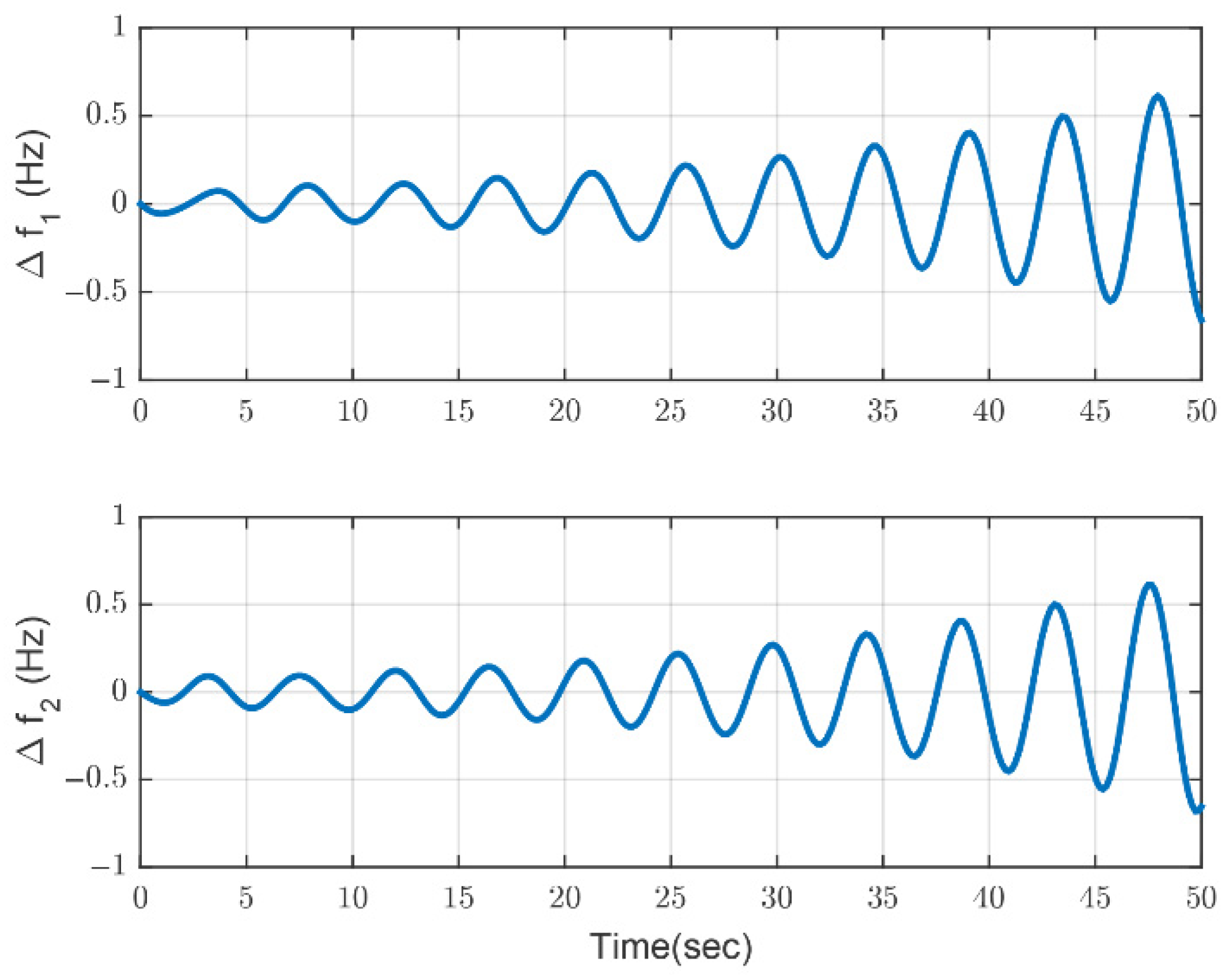
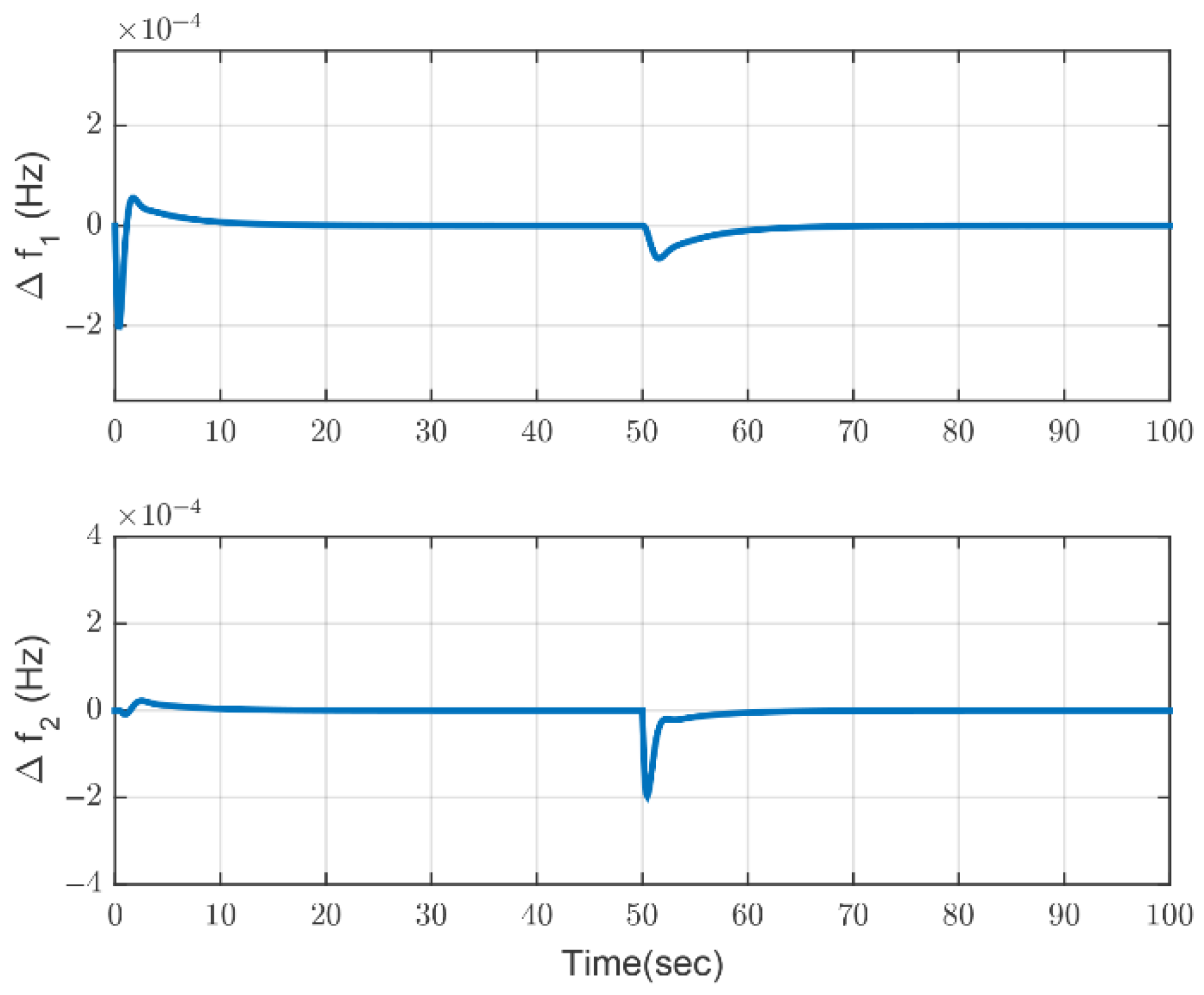
5. Simulation Results

In this section, the effectiveness and robustness of the proposed approach are demonstrated through simulation results of a delayed uncertain power system with two areas by consideration of valve position limitations. The system is shown in Figure 2 which in area 1, there are two generators and area 2 has four generators.

Table 1. Nominal values of model parameters.

Area	${\mathit{T}}_{\mathit{c}\mathit{h}\mathit{i}}\left(\mathit{s}\right)$	${\mathit{T}}_{\mathit{g}\mathit{i}}\left(\mathit{s}\right)$	${\mathit{R}}_{\mathit{i}}$	${\mathit{T}}_{\mathit{p}}$	${\mathit{K}}_{\mathit{p}}$	${\mathit{k}}_{\mathit{i}}$	${\mathit{B}}_{\mathit{i}}$	$\mathit{T}$
1	0.3	0.1	0.05	10	1	0.5	41	3
2	0.17	0.4	0.05	8	0.66	0.5	81.5	3

presents the nominal values of system parameters [16,17,29].

Moreover, in both control regions, time delays are adjusted as ${\tau }_1=0.5 \mathrm{s}$ and ${\tau }_2=0.5 \mathrm{s}.$

All simulations are performed on MATLAB software running on a computer with a 2.67 GHz Intel Core i5 CPU, 4GB RAM, and a 64-bit operation system. The computation complexity depends on the number of decision variables in the LMIs and the maximum order of LMI which are strongly linked to the delayed states [30].

The results of an event as a unit step change in the load demand with no extra control input are illustrated in Figure 4. The results show that the nonlinear uncertain delayed LFC system is unstable using predetermined local PI controllers $\left(\frac{K_i}{s}\right)$.

The parameters $\Delta P_{v{i}_{\min }}$ and are considered as 0.12 p.u. and −0.03 p.u., respectively. Furthermore, design parameters ${\xi }_1$ and ${\xi }_2$ are chosen as 0.47.

After solving the constrained optimization problem (22), the following feedback gains are obtained:

$$\begin{array}{l}{K}_1=\left[\begin{array}{ccccccccc}-6.6852& -0.1524& -0.0451& -0.5641& -0.019& -1.6628& -0.0292& -0.0783& -00604\\ -3.1283& -0.0501& -0.0129& -0.0241& -0.584& -12.6463& -0.1491& -0.1826& -0.6933\end{array}\right]\\ K_{d_1}=\left[\begin{array}{ccccccccc}-6.2511& -0.1426& -0.0422& -0.5296& -0.0138& -1.4892& -0.0266& -0.0723& -0.0524\\ -2.9809& -0.048& -0.0124& -0.0259& -0.5485& -11.8704& -0.14& -0.1719& -0.6509\end{array}\right]\\ \\ K_2=\left[\begin{array}{ccccccccc}-7.4708& -0.1813& -0.0264& -0.5945& 0.3277& 2.2583& 0.0187& -0.0207& 0.1924\\ -6.3227& -0.1443& -0.0191& -0.2322& -0.4728& -15.9433& -0.1858& -0.2348& -0.7837\end{array}\right]\\ K_{d_2}=\left[\begin{array}{ccccccccc}-7.2047& -0.1749& -0.0255& -0.5745& 0.3178& 2.1975& 0.0183& -0.0197& 0.187\\ -6.1283& -0.1399& -0.0185& -0.2251& -0.4564& -15.3798& -0.1793& -0.2268& -0.7563\end{array}\right]\\ \\ K_3=\left[\begin{array}{ccccccccc}-7.1772& -0.1646& -0.0491& -0.4241& -0.2616& -4.0832& -0.0579& -0.0582& -0.1952\\ -1.0961& -0.0197& -0.0056& 1.005& -1.3216& -7.9109& -0.104& -0.0889& -0.7647\end{array}\right]\\ K_{d_3}=\left[\begin{array}{ccccccccc}-6.6993& -0.1537& -0.0458& -0.4084& -0.2295& -3.7384& -0.0531& -0.0535& -0.174\\ -1.1008& -0.0202& -0.0057& 0.9358& -1.2392& -7.4423& -0.0979& -0.0838& 0.7175\end{array}\right]\\ \\ K_4=\left[\begin{array}{ccccccccc}-10.4211& -0.251& -0.036& -0.5611& -0.0069& -4.0349& -0.0579& -0.0649& -0.1088\\ -5.1781& -0.1273& -0.0188& 0.1786& -0.6879& -10.4642& -0.135& -0.1079& -0.5375\end{array}\right]\\ K_{d_4}=\left[\begin{array}{ccccccccc}-9.9989& -0.2408& -0.0345& -0.5401& -0.0041& -3.8448& -0.0552& -0.062& -0.1027\\ -5.0109& -0.1232& -0.0182& 0.1699& -0.6612& -10.0707& -0.1299& -0.0104& -0.517\end{array}\right]\end{array}$$

(26)

The main objective of the presented approach is to stabilize the outputs of the system (Δf₁, Δf₂) in presence of delays, parameter uncertainties, load disturbances, and valve position limits. Two kinds of load disturbances are assumed in this simulation, namely, unit and random step changes in load demands in areas 1 and 2. For the unit step change, load demand change assumes that the load demand change is 0.01 p.u. step changes in load demand of area 1 at the initial time and 0.01 p.u. step changes in load demand of area 2 at t = 50 s.

Figure 5, Figure 6 and Figure 7 show the fluctuations of frequency, mechanical power output, and tie-line power under the unit step load disturbances for the closed-loop LFC system with a fuzzy robust multi-objective H₂/H_∞ delayed feedback controller. It can be seen that the deviations in frequency, mechanical power output, and tie-line power reach desired points with suitable transient responses. Moreover, the corresponding control inputs are shown in Figure 8.

In another scenario, the random load demand change illustrated in Figure 9 is entered into both areas. The frequency, mechanical power, and tie-line power deviations of the closed-loop LFC system using the presented control structure step load disturbance randomly are shown in Figure 10, Figure 11 and Figure 12, respectively. Moreover, the control signals are shown in Figure 13. The results prove that the presented scheme could efficiently fulfill performance criteria, such as fast transient responses, load disturbance rejection, and robustness by considering all practical limitations.

Moreover, transient specifications of the closed-loop responses with the proposed method are compared with closed-loop responses obtained from other references. The comparison of numerical values of time domain specification for unit step load and random load demand changes are given in

Table 2. Comparison of transient specifications of the proposed approach with other existed works for unit step load demand change.

Parameter	Peak Overshoot	Peak Undershoot	Settling Time	Steady-State Error	Method
$\Delta f_1$	$0.0003$	$0.0037$	$13.38$	$5.21\times {10}^{-5}$
$\Delta f_2$	$0.0046$	$0.0041$	$17.64$	$3.67\times {10}^{-7}$
$\Delta P_{m1}$	$0.06$	$0.005$	$14.27$	-	[16]
$\Delta P_{m2}$	$0.043$	$0.016$	$20.86$	-
$\Delta P_{12}$	$0.0031$	$0.0019$	$17.43$	$1.52\times {10}^{-6}$
$\Delta f_1$	$0.0001$	$0.0003$	$12.92$	$3.57\times {10}^{-6}$
$\Delta f_2$	$0.0027$	$0.00025$	$18.68$	$2.11\times {10}^{-7}$
$\Delta P_{m1}$	$0.01$	$0.017$	$13.71$	-	[17]
$\Delta P_{m2}$	$0.013$	$0.0063$	$18.64$	-
$\Delta P_{12}$	$0.008$	$0.0076$	$17.88$	$5.44\times {10}^{-7}$
$\Delta f_1$	$5.54\times {10}^{-5}$	$0.0002$	$12.78$	$1.73\times {10}^{-9}$
$\Delta f_2$	$2.2\times {10}^{-5}$	$0.00019$	$20.09$	$9.43\times {10}^{-10}$
$\Delta P_{m1}$	$0.012$	$0.008$	$12.06$	-	Proposed method
$\Delta P_{m2}$	$0.0026$	$0.0078$	$18.13$	-
$\Delta P_{12}$	$0.0026$	$0.0024$	$18.58$	$7.23\times {10}^{-8}$

and

Table 3. Comparison of transient specifications of the proposed approach with other existed works for random load demand change.

Parameter	Peak Overshoot	Peak Undershoot	Settling Time	Steady-State Error	Method
$\Delta f_1$	$0.044$	$0.024$	$15.3$	$2.2\times {10}^{-5}$
$\Delta f_2$	$0.0061$	$0.023$	$17.55$	$5.78\times {10}^{-8}$
$\Delta P_{m1}$	$0.85$	$0.77$	$16.79$	-	[16]
$\Delta P_{m2}$	$0.51$	$0.37$	$17.3$	-
$\Delta P_{12}$	$0.3$	$0.22$	$20.42$	$8.58\times {10}^{-7}$
$\Delta f_1$	$0.038$	$0.01$	$16.24$	$1.02\times {10}^{-5}$
$\Delta f_2$	$0.007$	$0.018$	$16.2$	$3.97\times {10}^{-6}$
$\Delta P_{m1}$	$0.75$	$0.068$	$15.8$	-	[17]
$\Delta P_{m2}$	$0.42$	$0.32$	$18.37$	-
$\Delta P_{12}$	$0.28$	$0.2$	$19.33$	$7.74\times {10}^{-7}$
$\Delta f_1$	$0.023$	$0.0098$	$15.55$	$1.14\times {10}^{-7}$
$\Delta f_2$	$0.0059$	$0.012$	$14.98$	$6.21\times {10}^{-9}$
$\Delta P_{m1}$	$0.92$	$0.5$	$14.73$	-	Proposed method
$\Delta P_{m2}$	$0.35$	$0.3$	$16.89$	-
$\Delta P_{12}$	$0.24$	$0.19$	$18.96$	$7.54\times {10}^{-7}$

, respectively. Comparison results prove that the responses obtained from the proposed method have superiority compared to closed-loop responses employing other references.

Furthermore, in order to show the effectivity of the suggested scheme, this approach is compared with [16,17,18,19] in terms of considering load disturbance, parameter uncertainties, transmission delay, the nonlinearity of valve position limits, improving transient responses, and the ability of practical applications. This comparison is presented in

Table 4. Comparing the proposed approach with other existed works.

	[16]	[17]	[18]	[19]	Proposed Scheme
Load disturbance	Yes	Yes	Yes	Yes	Yes
Parameter uncertainties	No	Yes	No	Yes	Yes
Transmission delay	Yes	Yes	No	No	Yes
Nonlinearity of valve position limits	No	No	No	Yes	Yes
Delay-dependent controller	Yes	Yes	No	No	Yes
Reasonable and practical control signals	No	No	Yes	No	Yes

. The proposed method in this paper takes into account all design specifications which should be considered in real-world applications. Moreover, for emphasizing the efficiency of the proposed control system, a comparison with the existed controllers in terms of the norm values of the gain matrices is done and given in

Table 5. Comparison of the gain matrices norm values of the controllers.

	[16]	[17]	[18]	[19]	Proposed Scheme
${\Vert K\Vert }_2$	112.13	49.9	24.61	51.74	5.85
${\Vert K_d\Vert }_2$	9.64	39.94	-	-	12.77

. It can be seen from obtained results that the proposed controller is far more realizable than other existing controllers.

6. Conclusions

A robust ${\mathrm{H}}_2/{\mathrm{H}}_{\infty }$ delayed controller is proposed in this paper for LFC of an uncertain delayed multi-area power system with valve position limitations using an approximation of the nonlinear system using the TS fuzzy modelling. Then, a ${\mathrm{H}}_2/{\mathrm{H}}_{\infty }$ multi-objective delayed feedback controller was designed for attaining the robustness of the system. Finally, a fuzzy PDC scheme was used for the convergence of frequency deviations of the nonlinear power system. The main novelty of this paper is the designing of an LFC system with considering all theoretical and practical design specifications and limitations that had not been addressed before. Simulation results on a nonlinear uncertain delayed two-area power system confirm that the proposed method can efficiently alleviate the impacts of load disturbances, parametric variations, and transmission delays in presence of valve position limits on the governor. In addition, a comparison between transient specifications of responses shows that the proposed technique provided superior responses in terms of steady-state error, settling time, peak undershoot, and overshoot. Furthermore, a quantitative assessment in terms of the norm values of the gain matrices vindicated that the proposed controller scheme had a significant reduction in control signals which makes the proposed scheme highly desirable in practical applications. In future work, the proposed method for LFC of power systems will be investigated on renewable energy technologies such as wind turbines. Integration of renewable energy resources into power systems would be a challenging problem because of causing additional nonlinearities, new operational limitations, and undesirable dynamic behaviors which are left for further research. Moreover, due to the existence of thermal and mechanical constraints, the generation rate constraint imposes a practical constraint on the generation of power systems that are worth of being studied in the future.

References

1. Kundur, P. Power System Stability and Control; McGraw-Hill Books: New York, NY, USA, 1994; p. 581. [Google Scholar]
2. Sathya, M.R.; Ansari, M.M.T. Load frequency control using Bat inspired algorithm based dual mode gain scheduling of PI controllers for interconnected power system. Int. J. Electr. Power Energy Syst. 2015, 64, 365–374. [Google Scholar] [CrossRef]
3. Bevrani, H.; Hiyama, T. Robust decentralised PI based LFC design for time delay power systems. Energy Convers. Manag. 2008, 49, 193–204. [Google Scholar] [CrossRef]
4. Bevrani, H.; Mitani, Y.; Tsuji, K. Robust decentralised load-frequency control using an iterative linear matrix inequalities algorithm. IEE Proc. Gener. Transm. Distrib. 2004, 151, 347–354. [Google Scholar] [CrossRef] [Green Version]
5. Sharma, D.; Yadav, N.K. LFOPI controller: A fractional order PI controller based load frequency control in two area multi-source interconnected power system. Data Technol. Appl. 2020, 54, 323–342. [Google Scholar] [CrossRef]
6. Juang, C.F.; Lu, C.F. Load-frequency control by hybrid evolutionary fuzzy PI controller. IEE Proc. Gener. Transm. Distrib. 2006, 153, 196–204. [Google Scholar] [CrossRef]
7. Sudha, K.R.; Santhi, R.V. Robust decentralized load frequency control of interconnected power system with generation rate constraint using type-2 fuzzy approach. Int. J. Electr. Power Energy Syst. 2011, 33, 699–707. [Google Scholar] [CrossRef]
8. Shayeghi, H.; Shayanfar, H.; Malik, O. Robust decentralized neural networks based LFC in a deregulated power system. Electr. Power Syst. Res. 2007, 77, 241–251. [Google Scholar] [CrossRef]
9. Dahab, Y.A.; Abubakr, H.; Mohamed, T.H. Adaptive load frequency control of power systems using electro-search optimization supported by the balloon effect. IEEE Access 2020, 8, 7408–7422. [Google Scholar] [CrossRef]
10. Yang, M.; Wenlin, L.; Yuanwei, J. Decentralized load frequency variable structure control of multi-area interconnected power system. In Proceedings of the Chinese Control and Decision Conference (CCDC), Mianyang, China, 23–25 May 2011; IEEE: Piscataway, NJ, USA, 2011. [Google Scholar]
11. Dong, L.; Zhang, Y.; Gao, Z. A robust decentralized load frequency controller for interconnected power systems. ISA Trans. 2012, 51, 410–419. [Google Scholar] [CrossRef] [PubMed] [Green Version]
12. Delassi, A.; Arif, S.; Mokrani, L. Load frequency control problem in interconnected power systems using robust fractional PIλD controller. Ain Shams Eng. J. 2018, 9, 77–88. [Google Scholar] [CrossRef] [Green Version]
13. Vachirasricirikul, S.; Ngamroo, I. Robust LFC in a smart grid with wind power penetration by coordinated V2G control and frequency controller. IEEE Trans. Smart Grid 2014, 5, 371–380. [Google Scholar] [CrossRef]
14. Liu, X.; Zhang, Y.; Lee, K.Y. Robust distributed MPC for load frequency control of uncertain power systems. Control. Eng. Pract. 2016, 56, 136–147. [Google Scholar] [CrossRef]
15. Yu, X.; Tomsovic, K. Application of linear matrix inequalities for load frequency control with communication delay. IEEE Trans. Power Syst. 2004, 19, 1508–1515. [Google Scholar] [CrossRef]
16. Dey, R.; Ghosh, S.; Ray, G.; Rakshit, A. H load frequency control of interconnected power systems with communication delays. Int. J. Electr. Power Energy Syst. 2012, 42, 672–684. [Google Scholar] [CrossRef]
17. Sun, Y.; Li, N.; Zhao, X.; Wei, Z.; Sun, G.; Huang, C. Robust H load frequency control of delayed multi-area power system with stochastic disturbances. Neurocomputing 2016, 193, 58–67. [Google Scholar] [CrossRef]
18. Bensenouci, A.; Ghany, A.A. Mixed H/H2 with pole-placement design of robust LMI-based output feedback controllers for multi-area load frequency control. In Proceedings of the International Conference on Computer as a Tool, Warsaw, Poland, 9–12 September 2007; IEEE: Piscataway, NJ, USA, 2007. [Google Scholar]
19. Lee, H.J.; Park, J.B.; Joo, Y.H. Robust load-frequency control for uncertain nonlinear power systems: A fuzzy logic approach. Inf. Sci. 2006, 176, 3520–3537. [Google Scholar] [CrossRef]
20. Sharma, G.; Krishnan, N.; Arya, Y.; Panwar, A. Impact of ultracapacitor and redox flow battery with JAYA optimization for frequency stabilization in linked photovoltaic-thermal system. Int. Trans. Electr. Energy Syst. 2021, 31, e12883. [Google Scholar] [CrossRef]
21. Panwar, A.; Agarwal, V.; Sharma, G.; Sharma, S. Design of a novel AGC action for a linked hydro governing system. Electr. Power Compon. Syst. 2021, 49, 1201–1211. [Google Scholar] [CrossRef]
22. Kader, M.O.A.; Akindeji, K.T.; Sharma, G. A Novel Solution for Solving the Frequency Regulation Problem of Renewable Interlinked Power System Using Fusion of AI. Energies 2022, 15, 3376. [Google Scholar] [CrossRef]
23. Joshi, M.; Sharma, G.; Bokoro, P.N.; Krishnan, N. A Fuzzy-PSO-PID with UPFC-RFB Solution for an LFC of an Interlinked Hydro Power System. Energies 2022, 15, 4847. [Google Scholar] [CrossRef]
24. Zhang, Y.; Yang, T.; Tang, Z. Active fault-tolerant control for load frequency control in multi-area power systems with physical faults and cyber attacks. Int. Trans. Electr. Energy Syst. 2021, 31, e12906. [Google Scholar] [CrossRef]
25. Cheng, P.; Wang, H.; Stojanovic, V.; He, S.; Shi, K.; Luan, X.; Liu, F.; Sun, C. Asynchronous fault detection observer for 2-D Markov jump systems. In IEEE Transactions on Cybernetics; IEEE: Piscataway, NJ, USA, 2021. [Google Scholar]
26. Moon, Y.H.; Ryu, H.S.; Choi, B.K.; Cho, B.H. Modified PID load-frequency control with the consideration of valve position limits. In Proceedings of the IEEE Power Engineering Society. 1999 Winter Meeting (Cat. No. 99CH36233), New York, NY, USA, 31 January–4 February 1999; IEEE: Piscataway, NJ, USA, 1999; Volume 1, pp. 701–706. [Google Scholar]
27. Moon, Y.H.; Ryu, H.S.; Lee, J.G.; Song, K.B.; Shin, M.C. Extended integral control for load frequency control with the consideration of generation-rate constraints. Int. J. Electr. Power Energy Syst. 2002, 24, 263–269. [Google Scholar] [CrossRef]
28. Yu, L.; Chu, J. An LMI approach to guaranteed cost control of linear uncertain time-delay systems. Automatica 1999, 35, 1155–1159. [Google Scholar] [CrossRef]
29. Ahmadi, A.; Aldeen, M. An LMI approach to the design of robust delay-dependent overlapping load frequency control of uncertain power systems. Int. J. Electr. Power Energy Syst. 2016, 81, 48–63. [Google Scholar] [CrossRef]
30. Jin, L.; Zhang, C.K.; He, Y.; Jiang, L.; Wu, M. Delay-dependent stability analysis of multi-area load frequency control with enhanced accuracy and computation efficiency. IEEE Trans. Power Syst. 2019, 34, 3687–3696. [Google Scholar] [CrossRef]
Figure 1. A two-area system and its electrical equivalent circuit representation.
Energies 15 05525 g001
Figure 2. Block diagram of a two-area power system.
Energies 15 05525 g002
Figure 3. The typical mechanical structure of governor.
Energies 15 05525 g003
Figure 4. Frequency deviations in an LFC system without external control input.
Energies 15 05525 g004
Figure 5. Frequency deviations in the proposed LFC scheme during unit step load disturbance.
Energies 15 05525 g005
Figure 6. Deviation in mechanical power of the proposed LFC controller for unit step load disturbance.
Energies 15 05525 g006
Figure 7. Tie-line power deviations of proposed LFC scheme during the unit step load disturbance.
Energies 15 05525 g007
Figure 8. Control input for the unit step load disturbance.
Energies 15 05525 g008
Figure 9. Random load demand change entered to both areas.
Energies 15 05525 g009
Figure 10. Frequency deviation of the proposed LFC controller during a random step load disturbance.
Energies 15 05525 g010
Figure 11. Mechanical power output deviations of proposed LFC controller for random step load disturbance.
Energies 15 05525 g011
Figure 12. Tie-line power deviations of proposed LFC controller for the random step load disturbance.
Energies 15 05525 g012
Figure 13. Control input for the random step load disturbance.
Energies 15 05525 g013