
Time-Decoupling Layered Optimization for Energy and Transportation Systems under Dynamic Hydrogen Pricing


Abstract
:1. Introduction
- (1)
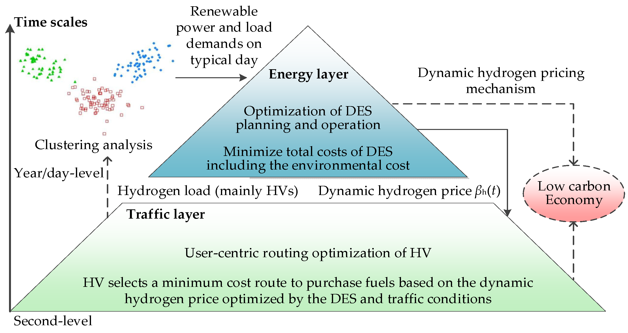
- Layered optimization of energy and transportation systems: confronted with the increasing penetration of renewable energy and HVs, a time-decoupling layered optimization strategy is proposed to realize the low-carbon economic operation of energy and transportation systems.
- (2)
- DES planning and operation optimization based on dynamic hydrogen pricing. A novel dynamic hydrogen pricing mechanism is proposed and incorporated into the optimization of DES planning and operation, which will promote hydrogen production using renewable power and minimize the DES operation cost.
- (3)
- User-centric routing optimization of HVs. On the basis of the dynamic hydrogen price optimized by the DES and the traffic condition on roads, the proposed user-centric routing optimization method can select a minimum cost route (MCR) for HVs to purchase fuels from a DES with low-cost and/or low-carbon hydrogen.
2. Time-Decoupling Layered Optimization Strategy
3. Energy Layer: Optimization of DES Planning and Operation
3.1. System Structure of DES
3.2. Optimization Model
- Objective Function
- The construction cost is represented by (2)–(4):
- The operation and maintenance cost is shown in (5):
- The environmental cost can be calculated by (6):
- The transaction cost is described in (7):
- 2.
- Equipment Constraints
- Electric boiler (EB):
- Electric cooling (EC):
- Electrolysis (Ele):
- Storage equipment (including electrical (EES)/thermal (TES)/hydrogen (HES) energy storage corresponding to d = 4, 5, and 6):
- 3.
- System Constraints of DES
- Equipment selection:
- Transaction power with the utility grid:
- Hydrogen sale price:
- Power balance (including electricity, heat, cooling, and hydrogen balance):
4. Traffic Layer: User-Centric Path Optimization of HVs
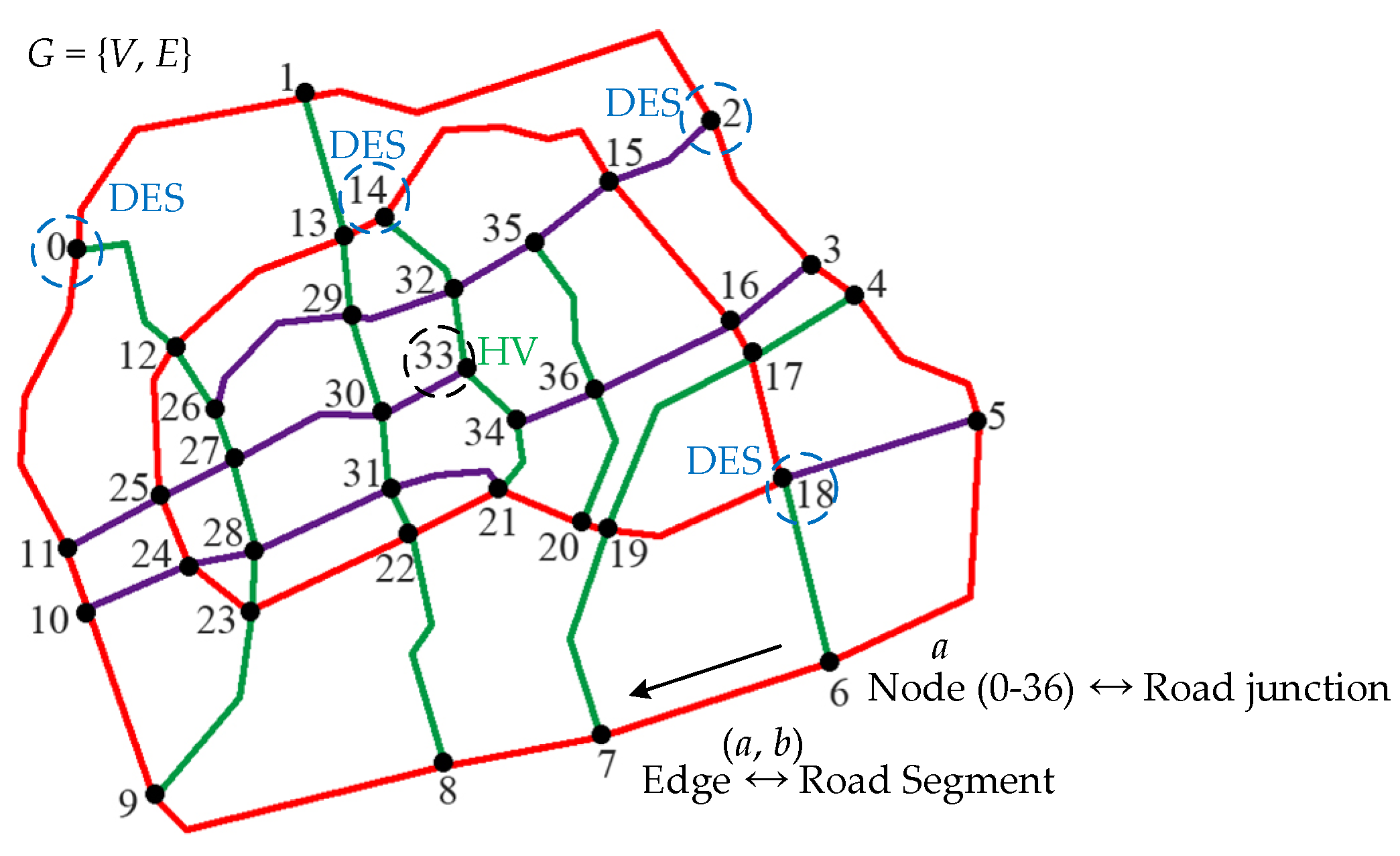
4.1. Graph Model of Traffic Roads
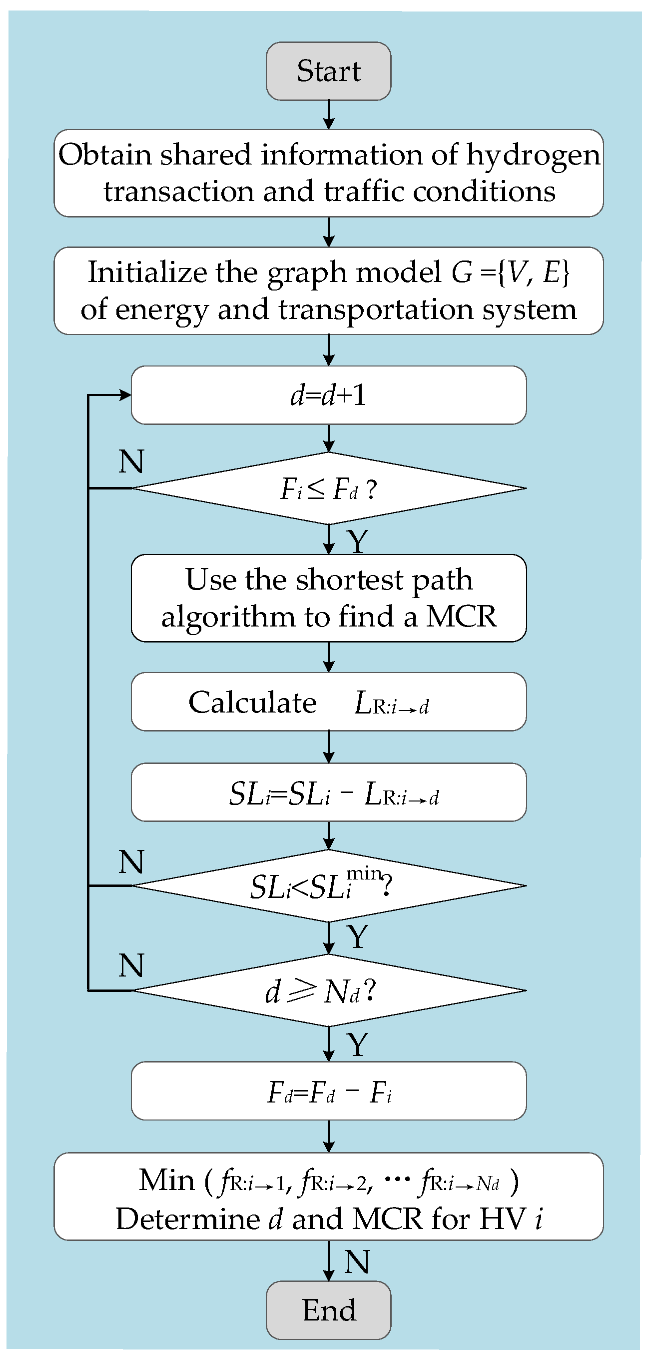
4.2. Routing Optimization
- Selection of MCR
- 2.
- Transaction Constraints
- 3.
- Traffic Constraints
5. Simulation Results and Analysis
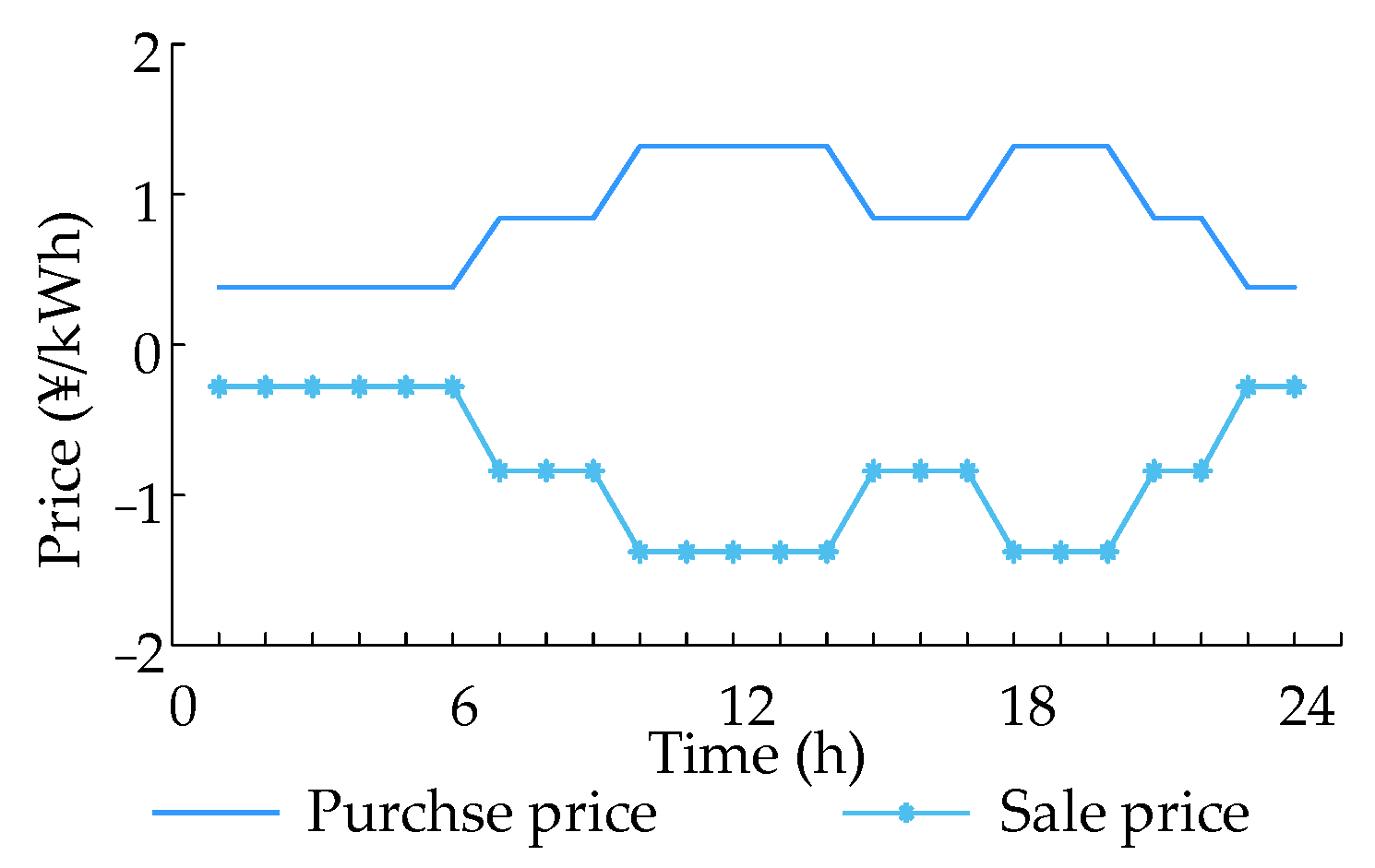
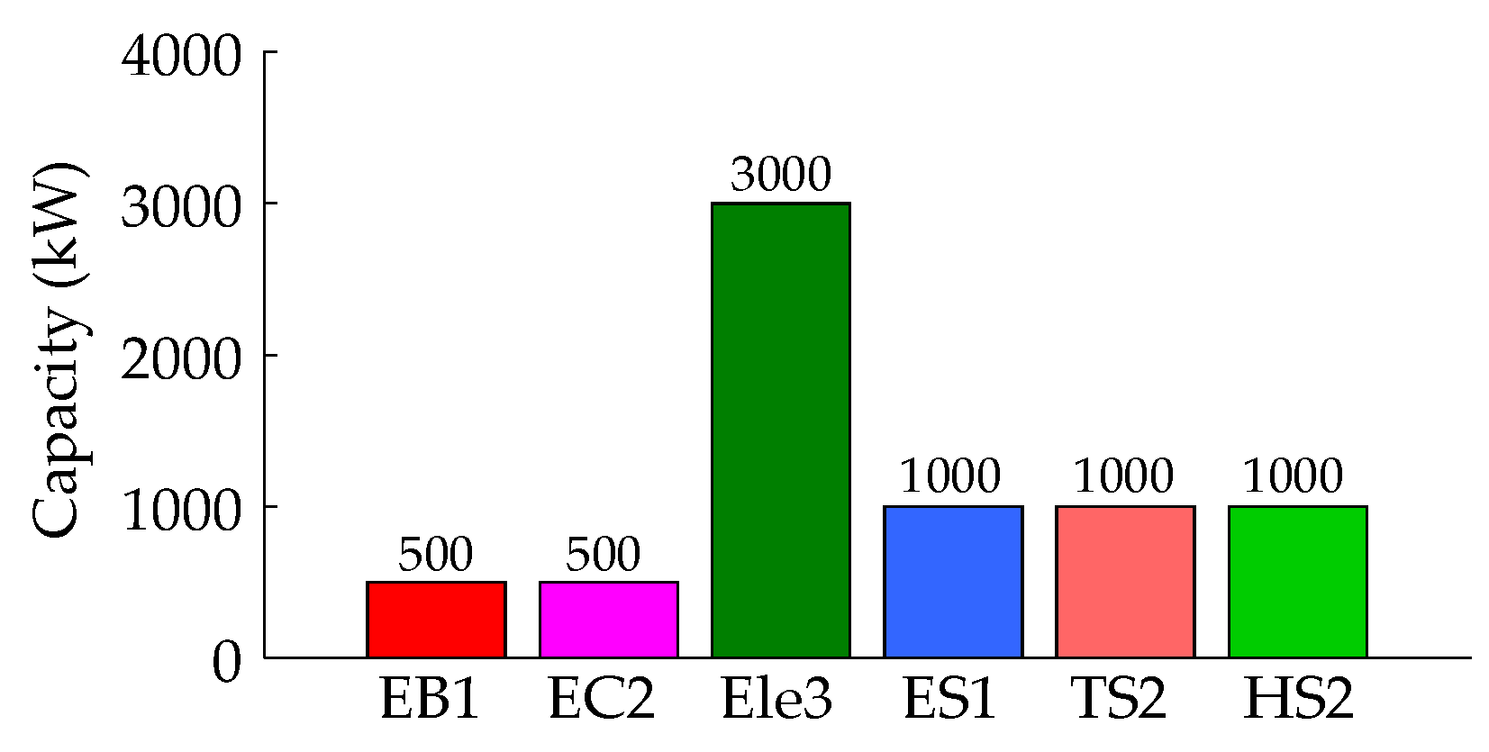
5.1. Energy Layer: Optimization of DES Planning and Operation
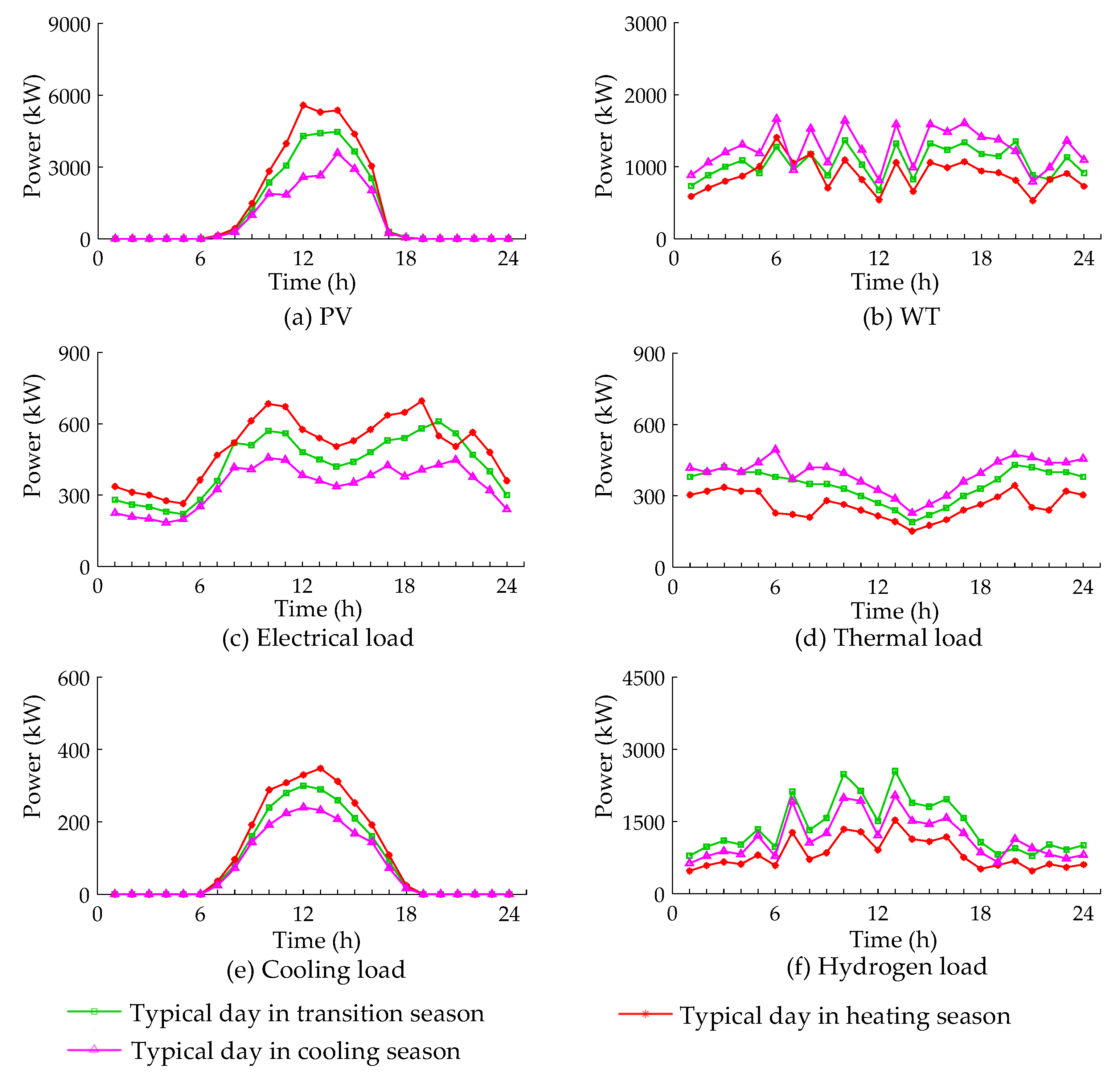
- Basic Data
- 2.
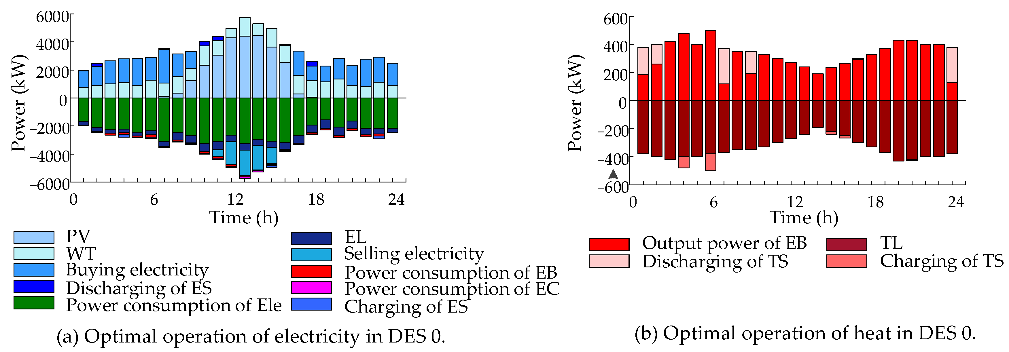
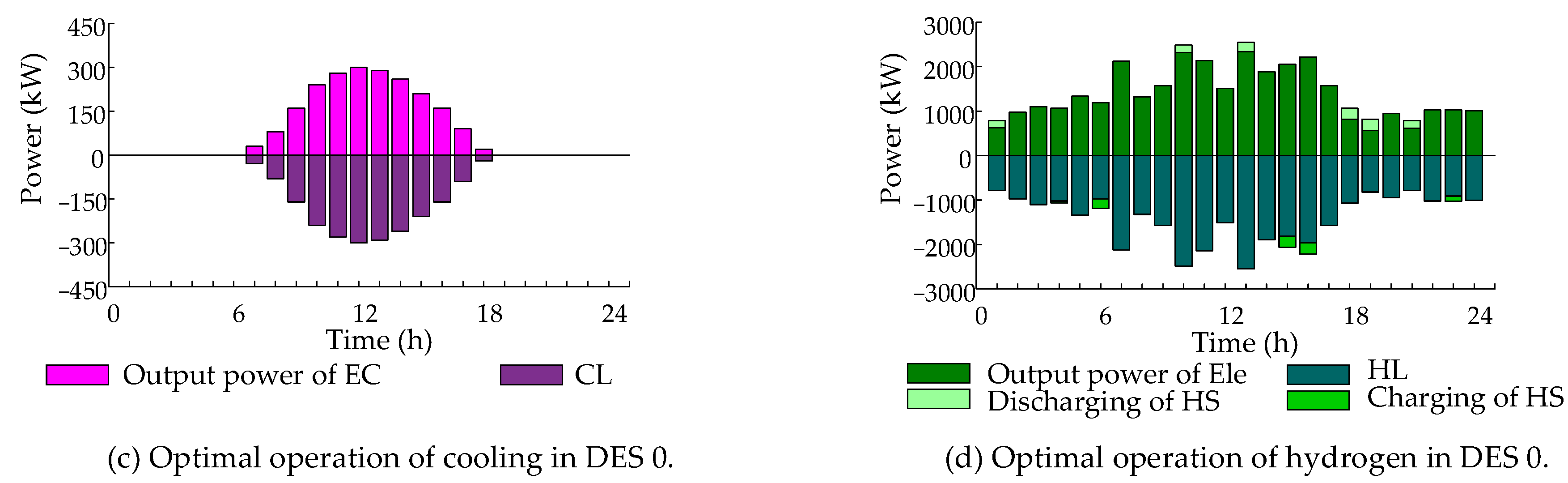
- Optimal Results
- Operation Optimization in DES 0:
- Dynamic Hydrogen Pricing:
- Comparison with Fixed Hydrogen Price:
5.2. Traffic Layer: User-Centric Routing Optimization of HVs
- Basic Data
- 2.
- Optimal Results
- Influence of the Road Direction:
- Influence of the Vehicle Flow on Roads:
- Influence of the Dynamic Hydrogen Price (compared with the fixed hydrogen price):
6. Conclusions
Author Contributions
Funding
Institutional Review Board Statement
Informed Consent Statement
Conflicts of Interest
Abbreviations
| DES | Distributed energy station |
| HV | Hydrogen-powered vehicle |
| EV | Electric vehicle |
| MCR | Minimum-cost route |
| WT | Wind turbine |
| PV | Photovoltaics |
| EB | Electric boiler |
| EC | Electric cooling |
| Ele | Electrolysis |
| ES | Electrical storage |
| TS | Thermal storage |
| HS | Hydrogen storage |
| EL | Electrical load |
| TL | Thermal load |
| CL/HL | Cooling/hydrogen load |
References
- Xia, F.; Rahim, A.; Kong, X.; Wang, M.; Cai, Y.; Wang, J. Modeling and Analysis of Large-Scale Urban Mobility for Green Transportation. IEEE Trans. Ind. Inform. 2018, 14, 1469–1481. [Google Scholar] [CrossRef]
- Liu, T.; Yu, H.; Guo, H.; Qin, Y.; Zou, Y. Online Energy Management for Multimode Plug-In Hybrid Electric Vehicles. IEEE Trans. Ind. Inform. 2019, 15, 4352–4361. [Google Scholar] [CrossRef]
- Chan, C.C. The State of the Art of Electric, Hybrid, and Fuel Cell Vehicles. Proc. IEEE 2007, 95, 704–718. [Google Scholar] [CrossRef]
- Kendall, K.; Kendall, M.; Liang, B.; Liu, Z. Hydrogen vehicles in China: Replacing the Western Model. Int. J. Hydrogen Energy 2017, 42, 30179–30185. [Google Scholar] [CrossRef]
- Mendis, N.; Muttaqi, K.M.; Perera, S.; Kamalasadan, S. An Effective Power Management Strategy for a Wind–Diesel–Hydrogen-Based Remote Area Power Supply System to Meet Fluctuating Demands Under Generation Uncertainty. IEEE Trans. Ind. Appl. 2015, 51, 1228–1238. [Google Scholar] [CrossRef]
- Jooshaki, M.; Abbaspour, A.; Fotuhi-Firuzabad, M.; Moeini-Aghtaie, M.; Lehtonen, M. MILP Model of Electricity Distribution System Expansion Planning Considering Incentive Reliability Regulations. IEEE Trans. Power Syst. 2019, 34, 4300–4316. [Google Scholar] [CrossRef] [Green Version]
- Robledo, C.B.; Oldenbroek, V.; Abbruzzese, F.; van Wijk, A.J.M. Integrating a hydrogen fuel cell electric vehicle with vehicle-to-grid technology, photovoltaic power and a residential building. Appl. Energy 2018, 215, 615–629. [Google Scholar] [CrossRef]
- El-Taweel, N.A.; Khani, H.; Farag, H.E.Z. Hydrogen Storage Optimal Scheduling for Fuel Supply and Capacity-Based Demand Response Program Under Dynamic Hydrogen Pricing. IEEE Trans. Smart Grid 2019, 10, 4531–4542. [Google Scholar] [CrossRef]
- Khani, H.; El-Taweel, N.A.; Farag, H.E.Z. Supervisory Scheduling of Storage-Based Hydrogen Fueling Stations for Transportation Sector and Distributed Operating Reserve in Electricity Markets. IEEE Trans. Ind. Inform. 2020, 16, 1529–1538. [Google Scholar] [CrossRef]
- Liu, Z.; Wen, F.; Ledwich, G. Optimal Planning of Electric-Vehicle Charging Stations in Distribution Systems. IEEE Trans. Power Deliv. 2013, 28, 102–110. [Google Scholar] [CrossRef]
- Luo, C.; Huang, Y.-F.; Gupta, V. Stochastic Dynamic Pricing for EV Charging Stations With Renewable Integration and Energy Storage. IEEE Trans. Smart Grid 2018, 9, 1494–1505. [Google Scholar] [CrossRef]
- Xiao, Y.; Wang, X.; Pinson, P.; Wang, X. A Local Energy Market for Electricity and Hydrogen. IEEE Trans. Power Syst. 2018, 33, 3898–3908. [Google Scholar] [CrossRef] [Green Version]
- Yuan, W.; Huang, J.; Zhang, Y.J. Competitive Charging Station Pricing for Plug-In Electric Vehicles. IEEE Trans. Smart Grid 2015, 8, 627–639. [Google Scholar] [CrossRef]
- Ghosh, A.; Aggarwal, V. Control of Charging of Electric Vehicles Through Menu-Based Pricing. IEEE Trans. Smart Grid 2018, 9, 5918–5929. [Google Scholar] [CrossRef] [Green Version]
- Chau, C.-K.; Elbassioni, K.; Tseng, C.-M. Drive Mode Optimization and Path Planning for Plug-In Hybrid Electric Vehicles. IEEE Trans. Intell. Transp. Syst. 2017, 18, 3421–3432. [Google Scholar] [CrossRef] [Green Version]
- Dong, X.; Mu, Y.; Jia, H.; Wu, J.; Yu, X. Planning of Fast EV Charging Stations on a Round Freeway. IEEE Trans. Sustain. Energy 2016, 7, 1452–1461. [Google Scholar] [CrossRef]
- Chen, T.; Zhang, B.; Pourbabak, H.; Kavousi-Fard, A.; Su, W. Optimal Routing and Charging of an Electric Vehicle Fleet for High-Efficiency Dynamic Transit Systems. IEEE Trans. Smart Grid 2018, 9, 3563–3572. [Google Scholar] [CrossRef]
- Morlock, F.; Rolle, B.; Bauer, M.; Sawodny, O. Time Optimal Routing of Electric Vehicles Under Consideration of Available Charging Infrastructure and a Detailed Consumption Model. IEEE Trans. Intell. Transp. Syst. 2020, 21, 5123–5135. [Google Scholar] [CrossRef]
- Ammous, M.; Belakaria, S.; Sorour, S.; Abdel-Rahim, A. Joint Delay and Cost Optimization of In-Route Charging for On-Demand Electric Vehicles. IEEE Trans. Intell. Veh. 2020, 5, 149–164. [Google Scholar] [CrossRef]
- Khuller, S.; Malekian, A.; Mestre, J. To fill or not to fill: The gas station problem. ACM Trans. Alg. 2011, 7, 36. [Google Scholar] [CrossRef]
- Pourazarm, S.; Cassandras, C.G. Optimal Routing of Energy-Aware Vehicles in Transportation Networks With Inhomogeneous Charging Nodes. IEEE Trans. Intell. Transp. Syst. 2018, 19, 2515–2527. [Google Scholar] [CrossRef]
- Zhang, H.; Qi, W.; Hu, Z.; Song, Y. Planning hydrogen refueling stations with coordinated on-site electrolytic production. In Proceedings of the 2017 IEEE Power & Energy Society General Meeting (PESGM), Chicago, IL, USA, 16–20 July 2017; pp. 1–5. [Google Scholar]
- Tao, Y.; Qiu, J.; Lai, S.; Zhang, X.; Wang, G. Collaborative Planning for Electricity Distribution Network and Transportation System Considering Hydrogen Fuel Cell Vehicles. IEEE Trans. Transp. Electrif. 2020, 6, 1211–1225. [Google Scholar] [CrossRef]
- Zhao, T.; Li, Y.; Pan, X.; Wang, P.; Zhang, J. Real-Time Optimal Energy and Reserve Management of Electric Vehicle Fast Charging Station: Hierarchical Game Approach. IEEE Trans. Smart Grid 2018, 9, 5357–5370. [Google Scholar] [CrossRef]
- Long, T.; Jia, Q.-S. Joint Optimization for Coordinated Charging Control of Commercial Electric Vehicles Under Distributed Hydrogen Energy Supply. IEEE Trans. Control Syst. Technol. 2022, 30, 835–843. [Google Scholar] [CrossRef]
- Yang, Q.; Sun, S.; Deng, S.; Zhao, Q.; Zhou, M. Optimal Sizing of PEV Fast Charging Stations With Markovian Demand Characterization. IEEE Trans. Smart Grid 2019, 10, 4457–4466. [Google Scholar] [CrossRef]
- de Quevedo, P.M.; Munoz-Delgado, G.; Contreras, J. Impact of Electric Vehicles on the Expansion Planning of Distribution Systems Considering Renewable Energy, Storage, and Charging Stations. IEEE Trans. Smart Grid 2019, 10, 794–804. [Google Scholar] [CrossRef]
- Yao, W.; Chung, C.Y.; Wen, F.; Qin, M.; Xue, Y. Scenario-Based Comprehensive Expansion Planning for Distribution Systems Considering Integration of Plug-in Electric Vehicles. IEEE Trans. Power Syst. 2016, 31, 317–328. [Google Scholar] [CrossRef]
- Li, Z.; Guo, Q.; Sun, H.; Wang, J. Coordinated Economic Dispatch of Coupled Transmission and Distribution Systems Using Heterogeneous Decomposition. IEEE Trans. Power Syst. 2016, 31, 4817–4830. [Google Scholar] [CrossRef]
- Guerrero, J.M.; Chandorkar, M.; Lee, T.-L.; Loh, P.C. Advanced Control Architectures for Intelligent Microgrids—Part I: Decentralized and Hierarchical Control. IEEE Trans. Ind. Electron. 2013, 60, 1254–1262. [Google Scholar] [CrossRef] [Green Version]
- Cheng, C.; Peng, C.; Zhang, T. Fuzzy K-Means Cluster Based Generalized Predictive Control of Ultra Supercritical Power Plant. IEEE Trans. Ind. Inform. 2021, 17, 4575–4583. [Google Scholar] [CrossRef]
- Huang, W.; Du, E.; Capuder, T.; Zhang, X.; Zhang, N.; Strbac, G.; Kang, C. Reliability and Vulnerability Assessment of Multi-Energy Systems: An Energy Hub Based Method. IEEE Trans. Power Syst. 2021, 36, 3948–3959. [Google Scholar] [CrossRef]
- Wu, Q.H.; Qin, Y.J.; Wu, L.L.; Zheng, J.H.; Li, M.S.; Jing, Z.X.; Zhou, X.X.; Wei, F. Optimal operation of integrated energy systems subject to the coupled demand constraints of electricity and natural gas. CSEE J. Power Energy Syst. 2019, 6, 444–457. [Google Scholar] [CrossRef]
- Wang, W.; Huang, S.; Zhang, G.; Liu, J.; Chen, Z. Optimal Operation of an Integrated Electricity-heat Energy System Considering Flexible Resources Dispatch for Renewable Integration. J. Mod. Power Syst. Clean Energy 2021, 9, 699–710. [Google Scholar] [CrossRef]
- Yang, W.; Liu, W.; Chung, C.Y.; Wen, F. Coordinated Planning Strategy for Integrated Energy Systems in a District Energy Sector. IEEE Trans. Sustain. Energy 2020, 11, 1807–1819. [Google Scholar] [CrossRef]
- Chen, J.; Zhang, W.; Li, J.; Zhang, W.; Liu, Y.; Zhao, B.; Zhang, Y. Optimal Sizing for Grid-Tied Microgrids With Consideration of Joint Optimization of Planning and Operation. IEEE Trans. Sustain. Energy 2018, 9, 237–248. [Google Scholar] [CrossRef]


| Conversion Equipment | Class | Capacity (kW) | Unit Construction Cost (RMB/kW) | Unit Operation Cost (RMB/kW) | Conversion Coefficient | Life (Year) |
|---|---|---|---|---|---|---|
| Electric cooling | EC1 | 100 | 800 | 0.008 | 3 | 20 |
| EC2 | 500 | 800 | 0.008 | 3 | 20 | |
| Electrolysis | Ele1 | 1000 | 12,000 | 0.16 | / | 10 |
| Ele2 | 2000 | 12,000 | 0.16 | / | 10 | |
| Ele3 | 3000 | 12,000 | 0.16 | / | 10 | |
| Electric boiler | EB1 | 500 | 1000 | 0.02 | 3 | 10 |
| EB2 | 1000 | 1000 | 0.02 | 3 | 10 | |
| EB3 | 1500 | 1000 | 0.02 | 3 | 10 |
| Storage Equipment | Class | Capacity (kW) | Unit Construction Cost (RMB/kW) | Unit Operation Cost (RMB/kW) | Self-Loss Coefficient | Charging/Discharging Efficiency |
|---|---|---|---|---|---|---|
| Electricity | ES1 | 1000 | 1700 | 0.0018 | 0.001 | 0.95 |
| ES2 | 2000 | 1700 | 0.0018 | 0.001 | 0.95 | |
| Heat | TS1 | 300 | 190 | 0.0016 | 0.01 | 0.85 |
| TS2 | 1000 | 190 | 0.0016 | 0.01 | 0.85 | |
| Hydrogen | HS1 | 500 | 1800 | 0.01 | 0.01 | 0.85 |
| HS2 | 1000 | 1800 | 0.01 | 0.01 | 0.85 |
| Time | Sale Price (RMB/kWh) | Sale Volume (kWh) | Time | Sale Price (RMB/kWh) | Sale Volume (kWh) |
|---|---|---|---|---|---|
| 1:00 | 1.7992 | 786 | 13:00 | 1.5276 | 2546.6 |
| 2:00 | 1.8354 | 974.6 | 14:00 | 1.5267 | 1886.4 |
| 3:00 | 1.7992 | 1100.4 | 15:00 | 1.5316 | 1807.8 |
| 4:00 | 1.7479 | 1021.8 | 16:00 | 1.5528 | 1965 |
| 5:00 | 1.9277 | 1336.2 | 17:00 | 1.6701 | 1572 |
| 6:00 | 1.7084 | 974.6 | 18:00 | 1.6529 | 1069 |
| 7:00 | 1.9820 | 2122.2 | 19:00 | 1.6210 | 817.4 |
| 8:00 | 1.6634 | 1320.5 | 20:00 | 1.6488 | 943.2 |
| 9:00 | 1.6069 | 1572 | 21:00 | 1.7087 | 786 |
| 10:00 | 1.5559 | 2483.8 | 22:00 | 1.8995 | 1021.8 |
| 11:00 | 1.5448 | 2137.9 | 23:00 | 1.7225 | 911.8 |
| 12:00 | 1.5248 | 1509.1 | 24:00 | 1.8256 | 1006.1 |
| Case | Scenario 1 | Scenario 2 | |
|---|---|---|---|
| Cost (RMB) | |||
| 15,642 | 15,642 | ||
| 5925 | 5912 | ||
| 501 | 496 | ||
| 18,708 | 18,158 | ||
| −9192 | −8448 | ||
| −50,508 | −56,166 | ||
| −18,925 | −24,406 | ||
| Time | Price (RMB/kg) | Volume (kg) | |
|---|---|---|---|
| 5:00 | HV 33 | / | 6.5 |
| DES 0 | 30.3034 | 85 | |
| DES 2 | 29.9277 | 80 | |
| DES 14 | 30.3034 | 85 | |
| DES 18 | 30.3018 | 75 | |
| 24:00 | HV 26 | / | 5 |
| DES 0 | 28.6984 | 64 | |
| DES 1 | 27.6075 | 63 | |
| DES 11 | 25.8060 | 60 | |
| Line | Distance (km) | Zero Flow Velocity (km/h) | Line | Distance (km) | Zero Flow Velocity (km/h) |
|---|---|---|---|---|---|
| (0,1) | 7.9 | 70 | (16,17) | 1.0 | 50 |
| (0,11) | 7.7 | 70 | (16,36) | 3.9 | 50 |
| (0,12) | 4.1 | 70 | (17,18) | 3.1 | 50 |
| (1,2) | 12.3 | 70 | (17,19) | 7.6 | 50 |
| (1,13) | 3.3 | 70 | (18,19) | 4.9 | 50 |
| (2,3) | 4.3 | 70 | (19,20) | 0.8 | 50 |
| (2,15) | 2.3 | 70 | (20,21) | 1.9 | 50 |
| (3,4) | 1.1 | 70 | (20,36) | 3.6 | 50 |
| (3,16) | 2.5 | 70 | (21,22) | 2.2 | 50 |
| (4,5) | 4.9 | 70 | (21,31) | 3.3 | 40 |
| (4,17) | 2.8 | 70 | (21,34) | 1.7 | 40 |
| (5,6) | 8.6 | 70 | (22,23) | 4.7 | 50 |
| (5,18) | 4.8 | 70 | (22,31) | 1.4 | 40 |
| (6,7) | 5.9 | 70 | (23,24) | 2.0 | 50 |
| (6,18) | 4.7 | 70 | (23,28) | 1.5 | 50 |
| (7,8) | 4.1 | 70 | (24,25) | 2.1 | 50 |
| (7,19) | 5.8 | 70 | (24,28) | 2.0 | 50 |
| (8,9) | 7.7 | 70 | (25,27) | 2.5 | 50 |
| (8,22) | 5.8 | 70 | (26,27) | 1.4 | 50 |
| (9,10) | 5.4 | 70 | (26,29) | 3.8 | 50 |
| (9,23) | 4.9 | 70 | (27,28) | 2.8 | 50 |
| (10,11) | 1.6 | 70 | (27,30) | 3.9 | 50 |
| (10,24) | 2.8 | 70 | (28,31) | 3.9 | 50 |
| (11,25) | 2.8 | 70 | (29,30) | 2.5 | 40 |
| (12,13) | 4.5 | 50 | (29,32) | 2.8 | 40 |
| (12,25) | 4.4 | 50 | (30,31) | 2.1 | 40 |
| (12,26) | 1.9 | 50 | (30,33) | 3.0 | 40 |
| (13,14) | 1.5 | 50 | (31,34) | 1.5 | 40 |
| (13,29) | 1.7 | 50 | (32,33) | 2.2 | 40 |
| (14,15) | 7.8 | 50 | (32,35) | 2.1 | 40 |
| (14,32) | 2.4 | 50 | (33,34) | 1.7 | 40 |
| (15,16) | 4.3 | 50 | (34,36) | 2.4 | 40 |
| (15,35) | 1.5 | 50 | (35,36) | 4.0 | 50 |
| Scenario | HV i | DES d | Minimum-Cost Route | TPC (RMB) | TAC (RMB) | Total Cost (RMB) | |
|---|---|---|---|---|---|---|---|
| 5:00 | 1 | 33 | 0 | 33→30→27→26→12→0 | 41.64 | 196.97 | 238.61 |
| 2 | 33→32→35→15→2 | 25.55 | 194.53 | 220.08 | |||
| 14 | 33→32→14 | 15.45 | 196.97 | 212.42 | |||
| 18 | 33→34→21→20→19→18 | 35.55 | 196.96 | 232.51 | |||
| 2 | 33 | 0 | 33→30→27→26→12→0 | 41.64 | 196.97 | 238.61 | |
| 2 | 33→32→35→15→2 | 25.55 | 194.53 | 220.08 | |||
| 14 | 33→32→29→13→14 | 28.35 | 196.97 | 225.32 | |||
| 18 | 33→34→21→20→19→18 | 35.55 | 196.96 | 232.51 | |||
| 24:00 | 1 | 26 | 0 | 26→12→0 | 14.49 | 143.49 | 157.98 |
| 1 | 26→29→13→1 | 23.57 | 138.04 | 161.61 | |||
| 11 | 26→27→25→11 | 17.70 | 129.03 | 146.73 | |||
| 2 | 26 | 0 | 26→12→0 | 14.49 | 143.49 | 157.98 | |
| 1 | 26→29→13→1 | 23.57 | 138.04 | 161.61 | |||
| 11 | 26→27→25→24→10→11 | 27.43 | 129.03 | 156.46 | |||
| 3 | 26 | 0 | 26→12→0 | 14.49 | 143.42 | 157.91 | |
| 1 | 26→29→13→1 | 23.57 | 143.42 | 166.99 | |||
| 11 | 26→27→25→11 | 17.70 | 143.42 | 161.12 | |||
Publisher’s Note: MDPI stays neutral with regard to jurisdictional claims in published maps and institutional affiliations. |
© 2022 by the authors. Licensee MDPI, Basel, Switzerland. This article is an open access article distributed under the terms and conditions of the Creative Commons Attribution (CC BY) license (https://creativecommons.org/licenses/by/4.0/).
Share and Cite
Guo, H.; Gong, D.; Zhang, L.; Mo, W.; Ding, F.; Wang, F. Time-Decoupling Layered Optimization for Energy and Transportation Systems under Dynamic Hydrogen Pricing. Energies 2022, 15, 5382. https://doi.org/10.3390/en15155382
Guo H, Gong D, Zhang L, Mo W, Ding F, Wang F. Time-Decoupling Layered Optimization for Energy and Transportation Systems under Dynamic Hydrogen Pricing. Energies. 2022; 15(15):5382. https://doi.org/10.3390/en15155382
Chicago/Turabian StyleGuo, Hui, Dandan Gong, Lijun Zhang, Wenke Mo, Feng Ding, and Fei Wang. 2022. "Time-Decoupling Layered Optimization for Energy and Transportation Systems under Dynamic Hydrogen Pricing" Energies 15, no. 15: 5382. https://doi.org/10.3390/en15155382
APA StyleGuo, H., Gong, D., Zhang, L., Mo, W., Ding, F., & Wang, F. (2022). Time-Decoupling Layered Optimization for Energy and Transportation Systems under Dynamic Hydrogen Pricing. Energies, 15(15), 5382. https://doi.org/10.3390/en15155382