MLD–MPC for Ultra-Supercritical Circulating Fluidized Bed Boiler Unit Using Subspace Identification

Abstract

Before carbon capture and storage technologies can truly be promoted and applied, and nuclear or renewable energy power generation can become predominant, it is important to further develop more efficient and ultra-low emission USC units on the basis of leveraging the strengths of CFB technology. In view of this complex system with strong nonlinearity such as the boiler-turbine unit of a thermal power unit, the establishment of a model that is suitable for control is indispensable for the operation and the economics of the process. In this study the form of the nonlinear model after linearization at the steady-state point has been fully considered and an improved subspace identification method, which is based on the steady-state point deviations data, was proposed in order to identify a piecewise affine model. In addition, the construction of the excitation signal in practical applications has been fully considered. The identification results demonstrate that this method has a better adaptability to strong nonlinear systems. The identification normalized root mean square errors of each working condition were almost all less than 10%. On this basis, a framework that is widely applicable to complex system control has been established by combining with the mixed logic dynamic (MLD) model. The canonical form realization was performed in order to transfer the local models into the same state basis. The predictive control was carried out on the boiler-turbine system of a 660-MW ultra-supercritical circulating fluidized bed unit that was based on the above framework. The results indicate that the predictive control performance is closely related to the setting value of the ramp rate and, therefore, prove the effectiveness of the framework.

1. Introduction

In order to achieve the goal of “carbon emissions would peak by 2030 and be neutralized by 2060 [1,2,3], and the proportion of non-fossil energy in primary energy consumption will reach about 20%”, and considering that the installed capacity of clean energy will continue to increase substantially during the “14th Five-Year Plan” period in China, it is imperative to vigorously develop circulating fluidized bed (CFB) boiler units and to transform pulverized coal (PC) boiler units into CFB boiler units, which has been strongly supported by the government.

Compared to PC boilers, the CFB boiler has developed into one of the most successful clean coal combustion technologies, with strong fuel adaptability [4] and low pollution control cost [5]. However, at the current stage, most of China’s CFB units only have subcritical parameters, which have no obvious advantages in achieving lower coal consumption for power supply. At the end of 2018, 24 supercritical boiler units, including the Baima 600-MW CFB boiler, were put into operation. In addition, in early 2019, two projects with 660-MW ultra-supercritical (USC) CFB boilers have been approved and are under construction in China. One is the Weihe 660-MW USC CFB boiler project, which burns anthracite with high sulfur content in the Guizhou province. Another one is the Binchang 660-MW USC CFB boiler project, which burns slime, gangue, and raw coal in the Shanxi province [6]. The power generation efficiency of the supercritical units reaches 45–47% [7], which is about 2.5% higher than the subcritical units, while the USC units can reach 49% [8]. At the same time, the CO₂ and SO₂ emissions of the USC units can be reduced by 145 [g/kWh] and 0.4 [g/kWh], respectively [9]. Before carbon capture and storage technologies can truly be promoted and applied, and nuclear or renewable energy power generation can become predominant, it is important to further develop more efficient and ultra-low emission USC units on the basis of leveraging the strengths of CFB technology.

The operation control system is one of the main research topics of CFB units at present, especially in the period when the thermal power units are transformed from the main power supply to the basic power supply, providing deep peak shaving [10]. The frequent and large-scale variable operating conditions aggravate the nonlinear impact of the thermal power unit and put forward higher requirements for the control system of the unit. At the same time, the equipment retrofit and changes in the coal quality also will cause significant changes in the dynamic characteristics of the unit, which will increase the difficulty of the control of the unit [11]. First of all, as far as the boiler is concerned, the capacity and the bed material of the 660-MW USC CFB units is much larger than that of the 300-MW subcritical CFB units, which accounts for the increased thermal inertia. Secondly, the USC CFB boilers are once-through boilers. In comparison with drum boilers, the heat storage on the steam side is greatly reduced, the rigidity of the working medium is improved, and the dynamic process is accelerated. Therefore, a faster control speed, a shorter control period, and a stronger coordination are required. Finally, the increase in the amount of coal slime leads to large fluctuations in the quality of the blended coal, which is also an enormous challenge in regard to the increasingly strict tracking ability assessment of the automatic generation control (AGC) and the frequency regulation.

Due to the fact that few supercritical CFB boiler projects have been put into production, and moreover, the Binchang 660-MW USC CFB boiler project is planned to be put into operation in July 2022, the mature and stable operation control strategy of this type of unit has largely been an under-explored domain. The design of the coordinated control system of the supercritical CFB boiler units draws on the control strategy of the supercritical PC boiler units. There have been some studies involving the design and optimization of the coordinated control system of the subcritical CFB boiler units and the supercritical PC boiler units that have reported [12,13]. However, the following non-negligible issues still exist in the design of the coordinated control system of USC CFB boiler units: (1) The combustion characteristics of CFB boilers are not taken into consideration, and the “three inputs-three outputs” form is employed as the coordinated control system model. In fact, the coal particles are not directly or fully burned in the CFB boiler, instead of going through the complicated process [14,15,16], which results in the heat that is generated by the coal particles that are newly fed into the furnace being unable to satisfy all of the energy requirements of the boiler, while the heat that is released by the carbon combustion that is stored in the furnace is dominant. (2) Simplicity of the distributed control structure with PID technology limits the load control rate to be formidable to settle for the 1 [%/min] assessment index of the power grid. (3) The control strategy of PID + feedforward decoupling cannot achieve the anticipative effects, especially considering the problems of large thermal inertia and multi-variable coupling. As a result, the deep peak shaving potential of the unit is limited, the automatic generation control (AGC) rate and the accuracy are reduced, and parameters, such as the steam temperature and the pressure, fluctuate greatly.

Compared to the other advanced control methods, the reason why predictive control has great engineering application value is that it can predict the change in the controlled object, can move ahead of time, and can deal with both soft and hard constraints. For the nonlinear object of CFB boiler units, a direct method is to establish a nonlinear model of the object through mechanism analysis, and achieve the control goal through nonlinear predictive control. However, Zhu H [17] has pointed out that although nonlinear predictive control has the same principles as linear predictive control (i.e., model prediction, rolling optimization, feedback correction), the optimization problem has a large amount of calculation involved and cannot meet the requirements of real-time computing in the industrial processes.

Generally, the linear model of the controlled object is obtained by local linearization of the nonlinear model near the steady-state condition. However, it is important to establish an accurate nonlinear mechanism model (white box model) for the CFB boiler units. In practical applications, a hybrid model (gray box model) that combines the mechanism model and the data-driven model is mostly used. In the hybrid model, the unknown parameters are identified from the actual data. When the model is complicated, the essence of the multi-parameter identification may be able to solve the non-convex optimization problem, which will cause the model parameters to vary widely under different identification data, resulting in low model generalization ability. Moreover, the white box model and the gray box model are usually not suitable for the design and the implementation of the controller, due to the complex equations that are involved. Another way to obtain the linear model of the object system is through identification. The model identification method determines the model form. Several studies have documented that piecewise affine (PWA) models can be used in order to approximate nonlinear systems that do not exhibit discontinuous or switching behaviors with arbitrary accuracy [18,19,20]. Several identification methods that are used for the linear time-variant (LTI) system, such as the prediction error method (PEM), the instrumental variable method (IVM), and the least-squares method, are based on optimization ideas and the system parameters are obtained by minimizing the difference between the model output and the actual output. Such methods have the following drawbacks: (1) The iterative solution of the nonlinear optimization is complicated. (2) The non-convex optimization is sensitive to the initial values, resulting in easily falling into a local optimum. (3) It is difficult to apply these methods to multiple input and multiple output problems. In contrast, the subspace identification methods (SIM) combining system theory, linear algebra, and statistics directly identify the LTI model from the input and output data without optimization and iteration. In addition, by only using the simple linear algebra tools, the SIM have strong robustness without regard to algorithm convergence. The SIM have not only enjoyed tremendous development in the last 30 years in theory [21,22,23,24,25,26,27,28,29,30], but also have caught up unremittingly in their practical application. Navalkar ST et al. [31] have applied subspace identification technology to the control of wind power generation systems. In addition to this, the SIM have also been widely used in blast furnace ironmaking [32], in nuclear reactors [33], in seismic response monitoring [34], in damage assessment [35], and so on. However, the SIM cannot be directly applied to identify PWA models, due to the existence of affine terms. In this work, the steady-state point deviations of each working condition are used as the identification data in order to obtain the PWA model based on the SIM.

After obtaining the PWA model of the research object, another core issue of the multi-model approach that needs to be focused on is the “weighting/switching rules”, that is, the “model/controller combination”. The methods of model/controller combination in the multi-model methods can be divided into the following two types: (1) soft switching, in which the global model is obtained by weighting and summing the local linear models/controllers by weighting the coefficients; (2) hard switching, in which only one of the local linear models/controllers take effect at each sampling time, according to the switching conditions. There are quite a few methods of determining the weight coefficients that are critical in soft switching, including the Gaussian local model validity function [36], Bayesian weighting [37], the gap metric [38], the trapezoidal functions [39], and so on. Likewise, multitudes of researchers have studied the switching rules in hard switching, such as the predicted feedback control error [40], the estimation error [41], the output error [42], the value function [43], and so on. When using the soft switching methods, the system runs smoothly, and model/controller switching will not result in a large range of output jumps at the expense of low control accuracy and unprovable stability. When compared to soft switching, the disadvantage of hard switching is that a wide range of output jumps occur during model switching, which leads to system oscillation. Consequently, a mixed-logical dynamic (MLD) model is proposed as a combination method of the models that are described in this paper in order to avoid the serious consequences that are caused by soft or hard switching. The MLD model is mainly used in order to model the hybrid system, which is described by the interacting physical laws, the logical rules, and the operational constraints. Furthermore, the equivalence between the PWA model and the MLD model, or the other hybrid dynamical models, has been proved [44,45]. In recent years, a host of scholars have conducted in-depth research on the MLD theory. Mahboubi H et al. [46] have analyzed the complexity of the MLD model. Di Cairano S et al. [47] have developed a class of continuous-time hybrid dynamical models for the expansion of discrete-time MLD models. Relying on the energetic development of the theory, MLD modeling ideas have also been extensively used in practice. However, these practical applications mainly focus on transportation deployment [48,49], energy dispatch [50,51], sewage treatment [52], and welding [53]. According to the characteristics of the MLD model that are expressed by linear dynamic equations that are subject to linear mixed integer inequalities, and fully considering that various inequality constraints can be handled conveniently and effectively by model predictive control (MPC), the MLD–MPC method will be employed in order to control the boiler-turbine unit. Compared with the other multi-model predictive control algorithms, the MLD–MPC method demonstrates the following superiorities: (1) the approximate linear model set can ensure the closed-loop stability of the system; (2) since the linear sub-models work under a unified performance criteria, which makes the controlled variables become globally optimized in the optimization horizon, the global optimal performance of the system can be guaranteed; (3) the mixed integer programming problem can be solved simply, and it is promising to realize the real-time calculation; (4) it is beneficial to eliminate the problem of oscillation that is caused by models/controllers switching.

If the local models are combined by the MLD modelling method, there are still prominent problems, to which urgent solutions are required. The reason why it is almost impossible for the state variables of each local model to be on the same basis is that the state variables of the models, which are identified by using the subspace method, have no practical significance. The use of the MLD models that are composed of the local models with a different basis may contribute to infeasible solutions. In addition, it is most credible to base the switching criteria directly on the state variables. The idea of state transformation was first proposed [54,55] for piecewise linear systems and jump linear systems. However, the method cannot be directly extended to transform the same basis of the local linear model. In this work, all of the local models are transformed into an observable canonical form in order to establish the local models with same basis.

To sum up, one hand, the research on the coordinated control system of USC CFB units is imminent. On the other hand, a considerable number of scholars have conducted both theoretical and practical research on SIM and MLD models. However, the focus of most practical research was on other fields, instead of the USC CFB units. Moreover, a standard linear state space model, instead of the linear affine model, can be obtained directly by using the input and the output data based on SIM. In addition, there is much discussion on the theoretical construction requirements of the excitation signal for system identification, while very few studies involve the construction of the pragmatic excitation signal in practical applications.

In this article, which is based on the previous research content and objects about the SIM and the MLD–MPC, the novelties are listed as follows:

• The steady-state point deviations of each working condition are employed as the identification data;
• The PWA model of a 660-MW USC CFB boiler unit is developed using the SIM;
• The construction of the excitation signal for identification in practical applications is fully considered;
• The MLD–MPC method is exploited in order to realize the control of the 660-MW USC CFB boiler unit.

The remainder of the paper is organized as follows: Section 2 is devoted to describing the 660-MW USC CFB boiler unit and proposes the corresponding coordinated control issues. Section 3 introduces the overall framework of the complex system/process control and the related algorithms in detail, respectively. Section 4 takes data from the simulation laboratory of Chongqing University and uses the framework that has been mentioned in Section 3 to obtain the results of the predictive control for the boiler-turbine unit, then the results are summarized and analyzed. Section 5 provides the conclusions and the future directions of research.

2. Process Description

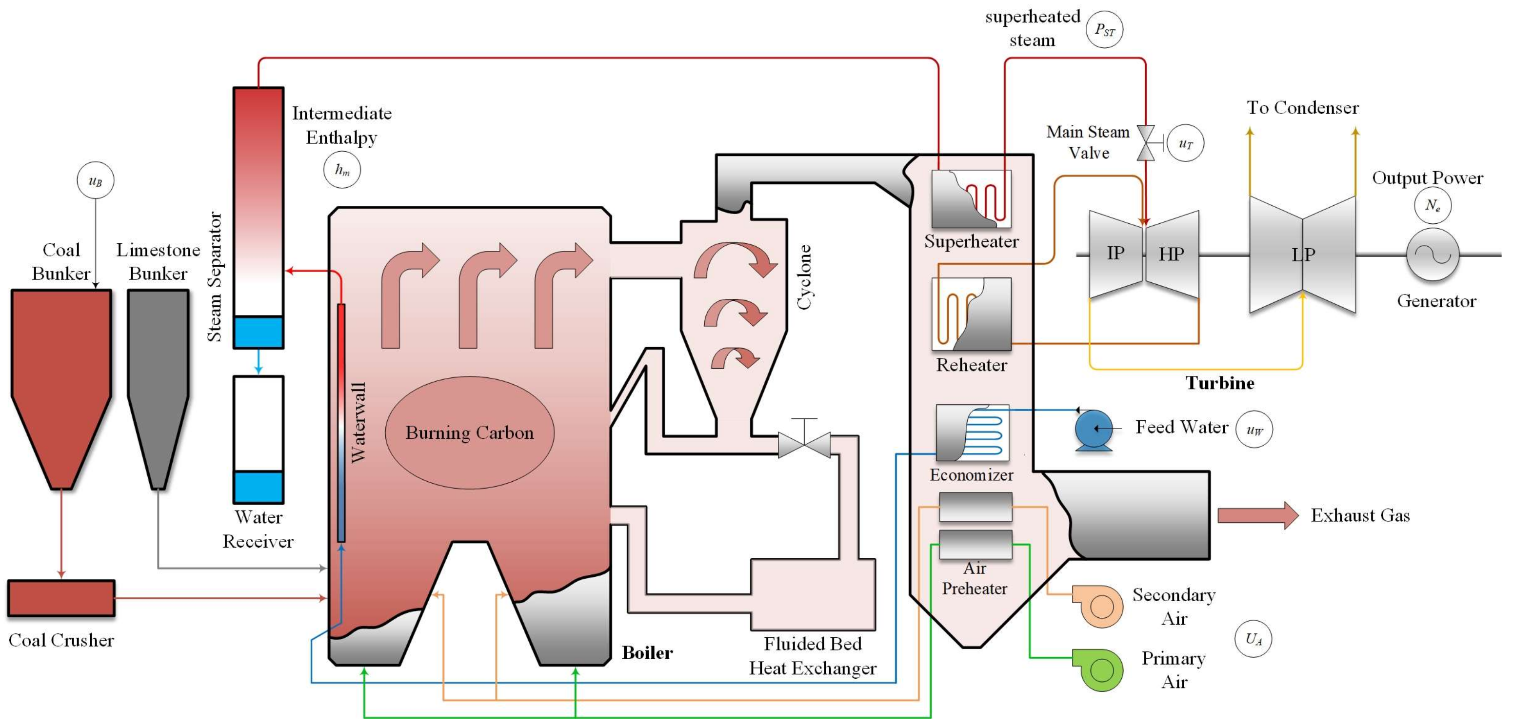
The USC CFB boiler unit is a nonlinear MIMO dynamic system that is characterized by large inertia, a long time lag, and is time-variant. The key control task of a thermal power unit is to regulate the output power of the unit in order to meet the load demand of the grid while maintaining various parameters within a given range. Unfortunately, it is arduous to simultaneously control the highly coupled variables in the boiler-turbine unit. Due to the diversity in the speed of the boiler-turbine unit in the energy conversion process, the fast and slow links have to be coordinated under the premise of considering the dynamic characteristics of the boiler and turbine in the meantime. This paper focuses on the research of the Weihe 660-MW USC CFB boiler unit, which is under construction. A schematic diagram of the boiler-turbine unit is shown in Figure 1.

The USC once-through boiler, which was designed by Oriental boiler Limited by Share Ltd., adopts a single furnace, trouser legs structure. The primary air enters the furnace from the air distribution plate at the bottom, so that the bed at the bottom of the furnace is in a fluidized state. Under the action of the primary air, the bed material moves upward from the bottom of the furnace. As the furnace rises, the upward moving speed of the solid gradually decreases, and moves downward near the furnace wall, forming a material circulation process in the furnace. The particles at the outlet of the furnace are captured by the cyclone and enter the external bed, then they return to the furnace from the returner, forming an external circulation of the material. In addition, the feed water, which is preheated by the economizer, enters the waterwall, in which the fluid absorbs the heat that is released by the combustion of the fuel and becomes saturated a mixture of steam and water. Then, the mixture is separated after entering the steam separator. Next, the steam leaves the separator and passes through the multi-stage superheaters in order to become superheated steam, preparing for entering the high-pressure turbine (HP). The steam from the HP passes through the intermediate-pressure turbine (IP) and the low-pressure turbine (LP) in turn, after being reheated by the multi-stage reheaters, and is then finally discharged into the condenser. Eventually, the steam that is working in the turbine drives the synchronous generator to produce the electric power. Finally, the fuel, the bed material, and the preheated air are sent into the furnace for cycle combustion by the coal bunker, the limestone bunker, and the forced-draft fan.

Compared with the PC boiler, the coal particles cannot be directly or fully burned. First, under the action of the fully fluidized high-temperature bed material, the coal particles are mixed with the high-temperature bed particles and are heated and dried. Then, the coal particles undergo pyrolysis with the burning of volatiles, and the coal particles are expanded, resulting in primary crushing. Finally, the remaining unburned carbon particles accumulate in the bed material in order to participate in the circulation and are sent back to the furnace through the cyclone for multiple combustion. It takes about 8 to 10 min to completely burn the carbon particles. If the heat storage of the burning carbon can be directly used to meet the load change in the unit, it will be more direct and rapid than changing the fuel command in order to respond to the load change. In the early stage of the load change, it is not essential to consider the corresponding relationship between the load, the wind, and the coal, and over-adjusting the air flow or fuel flow is permitted. In the middle of the load change, the heat balance principle is employed in order to gradually adjust the fuel flow and the air flow. The factors affecting the released heat of the furnace in the CFB boiler unit is illustrated in Figure 2.

As an indispensable part of the AGC system, the coordinated control system (CCS) accomplishes exactly maintaining the energy balance between the boiler and the turbine. The control-oriented model of boiler-turbine unit is obtained by simplifying the system-level model, rather than the component-level model of the specific equipment. A large number of works [56,57,58] have suggested that the model of the boiler-turbine unit can be simplified to a three inputs-three outputs (or even less) nonlinear model, on the condition that correctness is ensured. However, as mentioned above, the heat that is released by the burning carbon should be considered as the main heat of the boiler. The air flow has an enormous impact on the combustion of the burning carbon, which suggests that the main steam temperature and pressure respond to the change in air flow rapidly. If the combustion characteristics of the CFB boiler can be reasonably utilized in the control system, it is sufficient to improve the stability of the unit and the response rate of the unit to the load command. Consequently, a boiler-turbine unit model with a “four inputs-three outputs” form was established. The four input variables are the governor opening value of the steam turbine u_T, the fuel command u_B, the feed water flow u_W, and the air flow u_A. The three output variables include the output power N_e, the main steam pressure P_ST, and the intermediate enthalpy h_m. Compared to the steam parameters at the outlet of the superheater, the intermediate point temperature and enthalpy of the steam-water separator are more advanced, which can reflect the boiler’s energy fluctuation, the load change, and the coal-water ratio signals at the earliest stage, and the working fluid parameters in the steam-water separator are easy to measure. The CCS model that is composed of the main control system and the other sub-control systems is shown in Figure 3.

3. Proposed Methods

3.1. Overall Framework

As described above, the problem that is addressed in this article is to design a predictive controller for a complex system whose control-oriented model is difficultly built by mechanism analysis. The framework for solving the problem and methods that have been used in this work are shown in Figure 4.

In the model deployment stage, the linear models of the plant under different working conditions are established in the form of standard state space or as an affine item through the subspace identification method. In the model combination stage, the linear sub-models will be integrated by the MLD method, at the cost of introducing linear inequality constraints. In the predictive control stage, the predictive controller is designed by relying on the MLD model.

3.2. Subspace Identification

3.2.1. MON4SID Method

Subspace identification-related concepts and symbolic definitions are presented in Appendix A. The detailed process of the MON4SID algorithm refers to Appendix B.

3.2.2. SIM for Linear Affine Model Identification

It can be seen from the above theory that the subspace identification method is most suitable for the identification of the standard state space model, while the nonlinear model can be approximated by a set of linear affine models. The idea of applying the SIM to identify linear affine models originates from the traditional linearization method of nonlinear models on the basis of Taylor expansion. Suppose a discrete nonlinear dynamic system is represented as follows:

$$\begin{array}{c}{x}_{k+1}=f\left(x_k,u_k\right)+{\mathrm{w}}_k\\ y_k=g\left(x_k,u_k\right)+v_k\end{array}$$

(1)

where w_k∈R^l and v_k∈Rⁿ represent the process and measurement noise, respectively, which are independent of the input and output data. Linearizing at the steady-state point (x_s, u_s) using Taylor expansion, the following formula can be developed:

$$\begin{array}{c}{x}_{k+1}=f\left(x_s,u_s\right)+J_f^x\left|{}_{\left(x_s,u_s\right)}\right.\left(x_k-x_s\right)+J_f^u\left|{}_{\left(x_s,u_s\right)}\right.\left(u_k-u_s\right)+{\mathrm{w}}_k\\ y_k=g\left(x_s,u_s\right)+J_g^x\left|{}_{\left(x_s,u_s\right)}\right.\left(x_k-x_s\right)+J_g^u\left|{}_{\left(x_s,u_s\right)}\right.\left(u_k-u_s\right)+v_k\end{array}$$

(2)

where $J_f^x$ and $J_f^u$ represent Jacobian matrixes that demand f(x, u) on the x and u partial derivatives and $J_g^x$ and $J_g^u$ represent Jacobian matrixes that demand g(x, u) on the x and u partial derivatives. If we assume Δx_k = x_k − x_s, Δy_k = y_k − y_s and Δu_k = u_k − u_s, the above formulation can be transformed as follows:

$$\begin{array}{c}\Delta x_{k+1}=J_f^x\left|{}_{\left(x_s,u_s\right)}\right.\Delta x_k+J_f^u\left|{}_{\left(x_s,u_s\right)}\right.\Delta u_k+{\mathrm{w}}_k\\ \Delta y_k=J_g^x\left|{}_{\left(x_s,u_s\right)}\right.\Delta x_k+J_g^u\left|{}_{\left(x_s,u_s\right)}\right.\Delta u_k+v_k\end{array}$$

(3)

In terms of thermal power units, the steady-state point is generally the design condition, the deviation sequence is constructed according to the observation data and the steady-state point data, and four Jacobian matrixes (A, B, C, and D) can be calculated using SIM. After the system matrixes are obtained, Equation (2) is expanded and simplified to the linear affine model as follows:

$$\begin{array}{c}{x}_{k+1}=A{x}_k+B{u}_k+\underset{A\mathrm{f}fin{e}_f}{\underbrace{\left[-\left(A{x}_s+B{u}_s\right)+f\left(x_s,u_s\right)\right]}}+{\mathrm{w}}_k\\ y_k=C{x}_k+D{u}_k+\underset{A\mathrm{f}fin{e}_g}{\underbrace{\left[-\left(C{x}_s+D{u}_s\right)+g\left(x_s,u_s\right)\right]}}+v_k\end{array}$$

(4)

3.3. State Transformations

When the local models have been obtained, Equation (A2) can be applied to derive the state estimation at any time. However, the reason why it is almost impossible for the state variables of each local model to be on the same basis is that the state variables of the models, which are identified using the subspace method, have no practical significance. The switching criterion is determined by the output variable rather than time, which is related to the input variables and the evolution of the state variables, and as the result, the state of the switching points from the aspect of time scale will not be taken into account. In addition, the output variables are bound up with the observation matrix. When the feedthrough matrix is not considered, in order to obtain sub-models with the same basis, we must transform the sub-models into an observable canonical form as follows:

$${\mathrm{y}}_k=C{x}_k=\left[\begin{array}{cc}{\mathit{O}}_{l\times n-l}& {\mathit{I}}_{l\times l}\end{array}\right]x_k,$$

(5)

where I_l×l is the identity matrix of order l. This also means that the output variables are a subset of the state variables, which guarantees that the basis of the local sub-models is the same, and the output variables can be directly employed as switching criteria.

3.4. MLD Model

Hybrid systems are dynamic systems that involve the interaction of continuous dynamics (the state space sub-models under different operating conditions) and discrete dynamics (switching rules for different sub-models). There are a host of different methods of modeling for the hybrid system, namely the piecewise affine model, linear complementarity, and max-min-plus-scaling. The MLD model, which is described by interdependent physical laws, logic rules, and operation constraints, is also a kind of hybrid system model. Compared with other methods, the MLD method is more common and has less complexity.

A prominent characteristic of the MLD model is that it contains mixed integer inequalities, which are described by a set of linear dynamic inequalities. The establishment of mixed integer inequalities is based on the conversion of logical propositions to linear inequalities. In

Table 1. Fundamental conversion rules of logical propositions to linear inequalities [59].

Logical Proposition Type	Logical Expression	Linear Inequalities
Operation events caused by continuous dynamic characteristics	$\left[f\left(x\right)\le 0\right]\wedge \left[\delta =1\right]$	$f\left(x\right)-\delta \le -1+m\left(1-\delta \right)$
	$\left[f\left(x\right)\le 0\right]\vee \left[\delta =1\right]$	$f\left(x\right)\le M\delta$
	$\left[f\left(x\right)>0\right]$	$f\left(x\right)\ge \epsilon$
	$\left[f\left(x\right)\le 0\right]\Rightarrow \left[\delta =1\right]$	$f\left(x\right)\ge \epsilon +\left(m-\epsilon \right)\delta$
	$\left[f\left(x\right)\le 0\right]\iff \left[\delta =1\right]$	$\left\{\begin{array}{l}f\left(x\right)\le M\left(1-\delta \right)\\ f\left(x\right)\ge \epsilon +\left(m-\epsilon \right)\delta \end{array}\right.$
Multiplication of logical variables	${\delta }_3={\delta }_1{\delta }_2$	$\left\{\begin{array}{l}-{\delta }_1+{\delta }_3\le 0\\ -{\delta }_2+{\delta }_3\le 0\\ {\delta }_1+{\delta }_2-{\delta }_3\le 0\end{array}\right.$
Multiplication of logical variables and continuous variables	$z=\delta f\left(x\right)$	$\left\{\begin{array}{l}z\le M\delta \\ z\ge m\delta \\ z\le f\left(x\right)-m\left(1-\delta \right)\\ z\ge f\left(x\right)-M\left(1-\delta \right)\end{array}\right.$

, the fundamental conversion is summarized.

Where f is an affine function over a bounded set X of the input variable x; the constants m and M represent lower and upper bounds of the function f over X; δ∈{0,1} denote binary dummy variables; ε is an error tolerance, which is typically the machine precision; z is the auxiliary real variable. Therefore, using the basic rules, the system is modeled as an MLD through the following linear relations, and it should be emphasized that k, representing the time series, is used in brackets instead of subscript in order to avoid confusion:

$$\begin{array}{c}\left\{\begin{array}{l}x\left(k+1\right)=Ax\left(k\right)+B_{1}u\left(k\right)+B_2\delta \left(k\right)+B_{3}z\left(k\right)\\ y\left(k\right)=Cx\left(k\right)+D_{1}u\left(k\right)+D_2\delta \left(k\right)+D_{3}z\left(k\right)\\ E_2\delta \left(\mathrm{k}\right)+E_{3}z\left(\mathrm{k}\right)\le E_{1}u\left(\mathrm{k}\right)+E_{4}x\left(\mathrm{k}\right)+E_5\end{array}\right.\\ x={\left[\begin{array}{cc}{x}_c& x_l\end{array}\right]}^T,x_c\in R^{n_c},x_l\in {\left\{\begin{array}{cc}0& 1\end{array}\right\}}^{n_l}\\ y={\left[\begin{array}{cc}{y}_c& y_l\end{array}\right]}^T,y_c\in R^{p_c},y_l\in {\left\{\begin{array}{cc}0& 1\end{array}\right\}}^{p_l}\\ u={\left[\begin{array}{cc}{u}_c& u_l\end{array}\right]}^T,u_c\in R^{m_c},u_l\in {\left\{\begin{array}{cc}0& 1\end{array}\right\}}^{m_l}\end{array}$$

(6)

where x_c, y_c, and u_c denote continuous variables; x_l, y_l, and u_l denote discrete variables; A, B₁, B₂, B₃, C, D₁, D₂, D₃, E₁, E₂, E₃, E₄, and E₅ represent appropriate coefficient matrices.

3.5. MLD–MPC

The idea behind the design of the model’s predictive controller is mainly to establish a predictive model, and the design optimization criteria are based on the control task. Then, the predictive control variables are determined in order to optimize the performance criteria in the future prediction time domain, and repeated online calculation is carried out in order to optimize the control rate. It is noteworthy that only the first sample of the optimal sequence is applied to the plant at time step k, and at time step k + l, the whole optimization procedure is repeated with new plant measurements.

If k is the current time step, N is the prediction horizon, N_u is the control horizon, x(k) is the current state, x(k + j|k) is the predicted state at time step k + j under the influence of x(k), and input sequence uN_u k = {u(k), u(k + 1), …, u(k + N_u) and y(k + j|k), δ(k + j|k), z(k + j|k) are similarly defined, j = 1, 2, …, N, the optimal control problem, based on MLD, is established as follows:

$$\begin{array}{ll}\underset{\left\{u_k^{N_u}\right\}}{\min }J\left[u_k^{N_u},x\left(k\right)\right]& ={\displaystyle \sum _0^{Nu}{‖u\left(j\right)-u_r‖}_{Q_1}^P}+{\displaystyle \sum _0^{N-1}\left({‖y\left(k+j|k\right)-y_r‖}_{Q_2}^P+{‖x\left(k+j|k\right)-x_r‖}_{Q_3}^P\right.}\\ & +{‖\delta \left(k+j|k\right)-{\delta }_r‖}_{Q_4}^P+\left.{‖z\left(k+j|k\right)-z_r‖}_{Q_5}^P\right)\end{array}$$

(7)

$$s.t.\left\{\begin{array}{l}x\left(N|k\right)=x_e\\ x\left(j+1|k\right)=Ax\left(j|k\right)+B_{1}u\left(j\right)+B_2\delta \left(j|k\right)+B_{3}z\left(j|k\right)\\ y\left(j|k\right)=Cx\left(j|k\right)+D_{1}u\left(j\right)+D_2\delta \left(j|k\right)+D_{3}z\left(j|k\right)\\ E_2\delta \left(j|k\right)+E_{3}z\left(j|k\right)\le E_{1}u\left(j\right)+E_{4}x\left(j|k\right)+E_5\\ \dots \end{array}\right.,$$

(8)

where Q_i = QT i > 0, i = 1, …, 5, are the weighted matrices and u_r, y_r, x_r, δ_r, and z_r are the set values or referenced values. Moreover, other constraints, such as boundary constraints, can also be added to Equation (8).

According to the stability proof in Ref. [60], it is known that the optimal input sequence solved by Equations (7) and (8) can guarantee the stability of the MLD model.

The optimization problem is essentially a mixed integer programming problem, and the value of P makes the optimization problem more subdivided. When P = 1 or ∞, the problem is turned into a mixed integer linear programming (MILP) problem. When P = 2, the problem is turned into a mixed integer quadratic programming (MIQP) problem.

4. Simulation Experiments and Results

Generally speaking, the data that are used by performing identification should be collected from the actual physical plant. However, the use of a complicated excitation signal to fully stimulate the dynamic characteristics of the plant is in conflict with safety in actual production. In addition, there may be the intractable issue that the real physical system has not yet been put into operation, resulting in the inability to collect the data in the design stage. Consequently, using simulation models that are based on a mechanism instead of an actual plant in order to realize the data collection is an effective method. The industrial process simulation models that are required for implementing the data collection can be established manually by using flowsheet-based simulation environments or by other methods. In this paper, the mechanism model of the Weihe 660-MW USC CFB boiler unit, which was established by the simulation laboratory of Chongqing University, is the basis of collecting the data. The model form is derived from Ref. [12], and the unit parameters are re-tuned according to the design data. The accuracy of the simulation model dynamic characteristics have been validated by the designer [61].

4.1. Excitation Signal

The selection of a suitable excitation signal contributes to the identification result. For the SIM, how to apply the best input signal is still a thorny issue. However, it is universally acknowledged that a first-class excitation signal must meet several requirements. First of all, the excitation signal must be a quasi-stationary signal. Secondly, the system should be continuously and fully stimulated by the excitation signal. The last, but not least important requirement, is that the excitation signal must make the system outputs as uncorrelated as possible. The M sequence is a selectable excitation signal on account of the effortless implementation. Unfortunately, the spectral analysis shows that the M sequence contains the direct current component causing “net disturbance” to the identification system, which is not usually desired. The inverse M sequence overcomes this shortcoming and is more ideal than the M sequence.

When the excitation signal is applied in the actual system, the safety and the operability should be considered first. While applying it in the simulation system, it should be considered that it may cause a numerical calculation problem etc. Compared to the inverse M sequence, the simplicity and the security of the step signal make it more feasible to be used as an excitation signal. For a single-input system, a single-channel step signal can be directly used as the excitation signal. However, for multi-input systems, the reason why the step signal is not feasible to be used is that the identification algorithm may not be able to effectively separate the effects of each input on the output. Therefore, a non-simultaneous step multi-channel signal is proposed as the excitation signal. The design principle of a multi-channel step excitation signal is shown in Figure 5.

How to determine the step time point of each channel of the multi-input system is a crucial issue. In order to ensure that the dynamic characteristics of the system to the input change in each of the channels are fully reflected, the step time interval between the input of the different channels should be at least greater than that of the step response time of each output of the system. Therefore, before designing the excitation signal of the system, it is necessary to perform several step response experiments on the system in order to determine the step response time of the system to the input of each channel.

In this work, by taking full account of the pure delay and the step response time of the different inputs, a four-channel step signal has been designed as the excitation signal, with the purpose of adapting to the application in the actual system in six working conditions. The working conditions of the USC CFB unit are shown in

Table 2. The working conditions of the 660-MW USC CFB unit.

Working Conditions	Input Variables				Output Variables
	uB [kg/s]	uA [Nm3/s]	uW [kg/s]	uT [×100%]	Ne [MW]	PST [Mpa]	hm [kJ/kg]
BMCR	81.7	475.6	527.8	0.91	655.0	29.2	2753.0
BECR	78.1	458.2	513.5	0.92	620.9	27.3	2721.7
THA100%	72.2	423.2	470.5	0.84	575.4	27.7	2738.0
THA75%	55.0	321.3	360.7	0.82	422.9	20.9	2726.0
THA50%	37.6	225.7	241.2	0.82	279.7	13.8	2765.0
THA40%	31.6	221.3	200.4	0.81	233.1	11.7	2790.0

. In order to make the model fit the actual process as much as possible, and to prevent any model corruption that may be caused by the excessive step up/down of the inputs, the amplitudes of the governor opening value of the steam turbine u_T, the fuel command u_B, the feed water flow u_W, and the air flow u_A do not exceed 5% of the current stable value. Moreover, the four-channel inverse M sequence, whose time interval is 5000 s of the BMCR working conditions, is supposed to be control subject.

4.2. Identification Effects

The simulation is carried out with a sampling period of 1 s and 10⁵ data points are generated using the step signals in each working condition. Each sub-model is identified by the above illustrated MON4SID algorithm. The identification results with step excitation signals are shown in Figure 6. In addition, 1.55 × 10⁵ data points are generated using the inverse M sequence in the BMCR working condition, with purpose of comparison. The identification result with the inverse M sequence signals is illustrated in Figure 7. It can be acknowledged that the overall effect of the identification that is based on the step signals is more outstanding than that of the inverse M sequence. In fact, for the well-conditioned systems, the separation may not be clear-cut when the data for the model identification are generated from standard experiments with pseudo-random binary sequence (PRBS) inputs exciting the process, which will be identified. This is due to the fact that multiple inputs may change at the same time, which can result in the impossibility to determine the effect of a certain input on the output. In order to ensure the accuracy of the identification sub-models, we must restore the identification sub-model to the linear affine models according to the above method, and the inverse M sequence can be used as the verification signals and the outputs of the identification sub-models and the simulation model can be observed.

The normalized root mean square error (NRMSE) is designed as an indicator, which aims to achieve more intuitively measuring of the deviation between the identification model and the simulation model. Though there is no consistent approach of normalization in the literature, a common choice is the range (defined as the maximum value minus the minimum value) of the measured data. The NRMSE of the six working conditions is shown in

Table 3. The NRMSE of identification sub-models with the inverse M sequence verification signal in the six working conditions.

Working Conditions	Output Variables
	Ne [MW]	PST [Mpa]	hm [kJ/kg]
BMCR	6.48%	7.16%	5.17%
BECR	6.58%	6.81%	5.35%
THA100%	15.99%	10.05%	6.13%
THA75%	6.81%	7.03%	5.27%
THA50%	10.19%	8.26%	5.35%
THA40%	10.01%	9.13%	5.52%

. The NRMSE of the three output variables the in the six working conditions is almost lower than 10%, which shows that the high-fidelity of the local sub-models can be guaranteed.

4.3. State Transformations Effects

Transforming the local identification sub-models into the same basis can be achieved by transforming the sub-models into the same canonical form, such as the modal canonical form or the companion canonical form. Transforming the models into the form of Equation (5) means that the output variables can be directly employed as switching criteria, which is beneficial to MLD transformations.

4.4. MLD Transformation

In fact, it is completely feasible to perform MLD transformation on the small-scale sub-models manually. However, for the large-scale sub-models, especially the models that contain complicated logical deductions, manual MLD transformation is impossible. HYSDEL language that enables the transformation of information about the modeled system to the HYSDEL code is specifically used to describe the hybrid models. Once the HYSDEL code is available, it is then further processed for other purposes, such as the process simulation. Bemporad et al. [60] developed the HYSDEL compiler in 2004, which can transform the various models into an MLD model. It is for this reason that the HYSDEL compiler is applied in this work.

The prepared HYS file is directly generated through the HYSDEL compiler to the corresponding MLD model. The MLD model appears to be a linear model, but is essentially a nonlinear model, and its nonlinear characteristics are implicit in the binary variables. The MLD model is theoretically equivalent to the PWA model. In order to validate the MLD model, three sets of validation experiments were performed in this paper. The (a) experiment was performed in order to step from the BMCR to the THA40% working condition at 20,000 s. The (b) experiment was performed in order to step through the BMCR, the BECR, the THA100%, the THA75%, the THA50%, and then to the THA40% working conditions per 3000 s. The (c) experiment took a sine function with a frequency (8 × 10⁻⁴ [rad/s], 4 × 10⁻⁴ [rad/s], 8 × 10⁻⁴ [rad/s], 12 × 10⁻⁴ [rad/s]) and an amplitude (13, 60 [Nm³/s], 80 [kg/s], 0.025 [×100%]) as the input in order to perform the simulation at the steady-state point (u_B = 56.65, u_A = 348 [Nm³/s], u_W = 364.1 [kg/s], u_T = 0.865 [×100%]). The comparison results are shown in Figure 8. It is observed that the error between the output power, the main steam pressure of the MLD model, and simulation model is minimal. Although the intermediate enthalpy of the MLD model deviates from the simulation model at some of the working conditions, the change trends are absolutely the same. Therefore, the MLD model is capable of expressing the simulation model or the actual system.

4.5. Control Effects

According to control requirements, the performance criteria of the predictive control rolling optimization can be divided into the performance of the regulator and the tracker. Regulating the performance means that when the system deviates from the steady state due to a disturbance from the outside or from system noise, the system returns to the steady state by defining the index function. The tracking performance refers to the index function that the system outputs in order to track the reference trajectory. The above two criteria are both reflected in Equation (7). Since the model that was obtained by the SIM was performed with canonical form realization, this section of MLD-predictive control was mainly carried out based on the state variables criterion.

In addition to the inequalities that were introduced by establishing the MLD model, some actual constraints need to be declared. These constraints, and other parameters that are related to the predictive control, are illustrated in

Table 4. The related information of coordinated system predictive control.

	Expression	Value
Objective	$\begin{array}{ll}\underset{\left\{U_k^{N_u}\right\}}{min}J\left[U_k^{N_u},x\left(k\right)\right]& ={\displaystyle \sum _{j=0}^{Nu}{‖u\left(j\right)-u_{r\mathrm{ef}}‖}_{Q_1}^P}\\ & +{\displaystyle \sum _{j=0}^{N-1}\left({‖y\left(k+j|k\right)-y_{ref}‖}_{Q_2}^P+{‖x\left(k+j|k\right)-x_{ref}‖}_{Q_3}^P\right.}\\ & +{‖\delta \left(k+j|k\right)-{\delta }_{ref}‖}_{Q_4}^P+\left.{‖z\left(k+j|k\right)-z_{ref}‖}_{Q_5}^P\right)\end{array}$	$\begin{array}{c}P=2\\ Q_1=\left[\begin{array}{cccc}1& 0.1& 10& 10\end{array}\right]\\ Q_2=\left[\begin{array}{ccc}1& 0.2& 1\end{array}\right]\\ Q_3=0\\ Q_4=0\\ Q_5=0\\ N=20\\ N_u=1\end{array}$
MLD Constrains	$x\left(j+1|k\right)=Ax\left(j|k\right)+B_{u}u\left(j\right)+B_{\delta }\delta \left(j|k\right)+B_{z}z\left(j|k\right)$
	$y\left(j|k\right)=Cx\left(j|k\right)+D_{u}u\left(j\right)+D_{\delta }\delta \left(j|k\right)+D_{z}z\left(j|k\right)$
	$E_2\delta \left(j|k\right)+E_{3}z\left(j|k\right)\le E_{1}u\left(j\right)+E_{4}x\left(j|k\right)+E_5$
Actual Constrains	$u_{B\min }\le u_B\le u_{B\max },{\dot{u}}_{B\min }\le {\dot{u}}_B\le {\dot{u}}_{B\max }$	$\begin{array}{c}{u}_{B\min }=0\\ u_{B\max }=90\\ {\dot{u}}_{B\min }=-1[{\min }^{-1}]\\ {\dot{u}}_{B\max }=1[{\min }^{-1}]\end{array}$
	$u_{A\min }\le u_A\le u_{A\max },{\dot{u}}_{A\min }\le {\dot{u}}_A\le {\dot{u}}_{A\max }$	$\begin{array}{c}{u}_{A\min }=0{[\mathrm{Nm}}^3\cdot {\mathrm{s}}^{-1}]\\ u_{A\max }=500{[\mathrm{Nm}}^3\cdot {\mathrm{s}}^{-1}]\\ {\dot{u}}_{A\min }=-1{[\mathrm{Nm}}^3\cdot {\left(\mathrm{s}\cdot \min \right)}^{-1}]\\ {\dot{u}}_{A\max }=1{[\mathrm{Nm}}^3\cdot {\left(\mathrm{s}\cdot \min \right)}^{-1}]\end{array}$
	$u_{W\min }\le u_W\le u_{W\max },{\dot{u}}_{W\min }\le {\dot{u}}_W\le {\dot{u}}_{W\max }$	$\begin{array}{c}{u}_{W\min }=0[\mathrm{kg}\cdot {\mathrm{s}}^{-1}]\\ u_{W\max }=550[\mathrm{kg}\cdot {\mathrm{s}}^{-1}]\\ {\dot{u}}_{W\min }=-1[\mathrm{kg}\cdot {\left(\mathrm{s}\cdot \min \right)}^{-1}]\\ {\dot{u}}_{W\max }=1[\mathrm{kg}\cdot {\left(\mathrm{s}\cdot \min \right)}^{-1}]\end{array}$
	$u_{T\min }\le u_T\le u_{T\max },{\dot{u}}_{T\min }\le {\dot{u}}_T\le {\dot{u}}_{T\max }$	$\begin{array}{c}{u}_{T\min }=0[\%]\\ u_{T\max }=100[\%]\\ {\dot{u}}_{T\min }=-1[\%\cdot {\min }^{-1}]\\ {\dot{u}}_{T\max }=1[\%\cdot {\min }^{-1}]\end{array}$
	$P_{SS\min }\le P_{SS}\le P_{SS\max }$	$\begin{array}{c}{P}_{SS\min }=10\left[\mathrm{MPa}\right]\\ P_{SS\max }=32\left[\mathrm{MPa}\right]\end{array}$

.

Under the above constraints, 3000 [kW/min], 6000 [kW/min], 9000 [kW/min], and the step ramp rate were respectively used as the tracking objective of the predictive control, and the MIQP-based predictive control method was employed in order to obtain the predictive control results, which are shown in Figure 9.

The simulation result shows that when the unit begins to reduce the load, the fuel command and the air flow decrease. The heat release in the furnace decreases rapidly, resulting in the precipitously diminished intermediate enthalpy. In order to keep the intermediate enthalpy stable, the feed water flow is controlled in order to decrease it, and the intermediate enthalpy increases again. In addition, the governor opening value of the steam turbine is reduced in order to maintain the main steam pressure tracking effect. When the output power is reduced to the set value, the feed water flow and air flow rise so that the intermediate enthalpy drops to the set value. The dynamic process of the increasing load is opposite to that of the decreasing load.

When the ramp rate is small, the predictive control has a satisfactory performance, the output power deviation of the unit is low, the tracking effect of the main steam pressure is good, the intermediate enthalpy is stable, and the main steam pressure can be maintained at a normal level. When the ramp rate increases, the output power deviation of the unit increases gradually, the tracking effect of the main steam pressure becomes negative, the intermediate enthalpy fluctuates greatly, and the maximum value of the main steam pressure most likely exceeds that of the safety threshold, which is unfavorable for the operation of the unit. In general, the prediction controller of the 660-MW USC CFB unit that is based on the MLD model can successfully complete the task of coordinated control.

5. Conclusions and Future Work

In view of the complex system that is similar to the boiler-turbine unit of a thermal power unit, a multi-model predictive control method that is based on the SIM and the MLD model has been established. First, the SIM is employed in order to obtain the sub-models of the different operating conditions. Aiming at the disadvantages and the difficulty of the original SIM that was applied in the nonlinear model identification, the SIM that was based on the steady-state point deviations of the operating conditions was developed. The identification results have manifested the advantages of the method that is based on the steady-state point deviations. Then, multiple identification linear sub-models are transformed into the MLD models by introducing mixed integer linear inequalities. By combining the canonical form realization, the local models are transformed to the same basis, with the purpose of avoiding the problem of infeasible solutions in the MLD that are caused by different bases. The MLD model avoids the serious consequences that are caused by soft and hard switching, such as low control accuracy, unprovable stability, and a wide range of output jumps. Finally, the MIP problem is studied in order to lay the foundation for model predictive control based on the MLD model. Moreover, relying on the MLD model, the predictive control of the boiler-turbine system of a 660-MW USC CFB unit has been achieved and the desired control effects have been obtained.

The following major conclusions can be drawn from the simulation results:

• The SIM that was based on the steady-state point deviations of the operating conditions has a better adaptability to strong nonlinear systems. The identification normalized root mean square error of each of the working conditions were almost all less than 10%;
• The canonical form realization can be performed in order to transfer the local sub-models that were obtained by the SIM into the same state basis, which is a prerequisite for MLD model building;
• The SIM-based MLD–MPC method is effective for nonlinear system control;
• The set value of the unit ramp rate is a key factor affecting the performance of predictive control.

In this paper, the orders of the sub-models that were identified at the six operating conditions are exactly coincident, which provides a prerequisite for MLD model transformation. The MLD transformation for the sub-models of the different orders is more complicated. In addition, for some systems with high security requirements, the step signal may not be able to be applied in the actual plant, which may result in an unexpected accident. Smoother and safer multi-input excitation signals need to be designed in an actual system, while the identification signal is required in order to maintain a certain amplitude of excitation, trade-off must be deliberate. Finally, the meaningless state variables in the subspace identification model have an essential impact on the establishment of the logical relationships during the MLD transformation. The MLD model is likely to have no feasible solution due to over-constraint. Thus, the implementation of finding the inner relationship between the state variables of the subspace identification model is expected.