

Fault Detection and Classification in Transmission Lines Connected to Inverter-Based Generators Using Machine Learning


Abstract
:1. Introduction
- Only the positive current sequence is available for symmetrical and asymmetrical faults for fully converted renewable sources, like photovoltaic (PV) and type-4 wind turbines. The absence of a negative sequence current presents a challenge for the operation of protection devices that rely on negative sequence components. This challenge can be mitigated by specifying the requirement of negative sequence injection in the grid code using the decoupled sequence control mode of the inverter [2]. Furthermore, the difference between the phase angles of the negative-sequence voltage and current measured by a relay after an asymmetrical forward fault occurred was lesser for the system integrated with IBGs than the conventional power system with synchronous generators. This comparison was discussed in [3].
- The IBGs do not contribute to zero-sequence components because they are not grounded. In contrast, the coupling transformer grounding can obtain the zero-sequence component, a potent source supplying a high magnitude of zero-sequence current [4]. As a result, the zero-sequence component depends on the inverter, the IBG type, and the transformer connection [1].
- The stiffness of power systems with IBGs is reduced compared with conventional generation systems [5]. System stiffness (strength) can be evaluated by calculating the short circuit ratio (SCR). A power source is described as a weak system in the presence of IBGs (weak source means high SCR) [6]. IBGs have unique short circuit characteristics because of the integration of power electronics connected to the grid. When a short-circuit fault occurs, the inverter is switched to current-controlled mode (CCM), and the inverter behaves as a current source until the short-circuit fault is cleared by the protection devices [7]. Furthermore, the IBG output current increases as the voltage drops during faults to regulate it back to its P–Q setpoint. In this condition, the IBG becomes a current source [8].
- Adaptive protection schemes: They are defined as the online protection schemes used to adapt relay settings and characteristics according to the system’s current state [9]. Different adaptive schemes for microgrids were reviewed in [10]. The adaptive protection scheme depends on the communication infrastructure to exchange information in the form of measured network parameters such as voltage, current, and power. Therefore, the reliability of a viable adaptive protection scheme depends upon the redundancy of the communication system with the cybersecurity hazards [11,12]. Moreover, adaptive protection requires complex algorithms [13], which significantly increases the cost.
- Modification of fault current level: Fault contribution by IBGs could be modified by adding auxiliary devices on the IBG side to improve its performance during faults. Examples are crowbar rotor circuit (CRC), superconducting fault current limiter (SFCL), superconducting magnetic energy storage (SMES), and series dynamic braking resistor (SDBR). CRC was used to improve the stability of DFIG during faults and protect the rotor side converter [14]. SFCL aims to improve the low voltage fault ride-through (LV-FRT) capability [15]. SDBR was introduced to improve the LV-FRT capability of large wind turbines and the transient stability of DFIG during faults [16]. SMES stores the energy and handles its transfer caused by DFIG power fluctuation or grid fault to improve the LV-FRT [17]. As realized by the authors in [18], fault current-limiting devices introduced several challenges in the power system that require further analysis, such as interfering with communication lines, finding optimal design parameters, coordinated control design between these devices and other protective devices, feasibility analysis, field tests, and real-time grid operation.
- Meta-heuristic techniques: These are search algorithms capable of solving complex optimization problems. They include Genetic Algorithm, Annealing algorithm, Tabu Search, and Local Search algorithm. These techniques are high-level heuristics used to guide others for a better evolution in the search space [19]. Several researchers used the meta-heuristics for protection relay coordination to find the optimum relay setting according to the system topology. Dynamic and flexible protection approach considering different grid operation modes of microgrids for earth and phase overcurrent coordination using charged system search (CSS) and Teaching-Learning-Based Optimization Algorithm (TLBO) was proposed in [20]. The studied microgrid was connected to a distributed generator without defining the type of generator technology. The inefficient numerical search is always a limitation of these techniques, especially for high-dimensional problems [21].
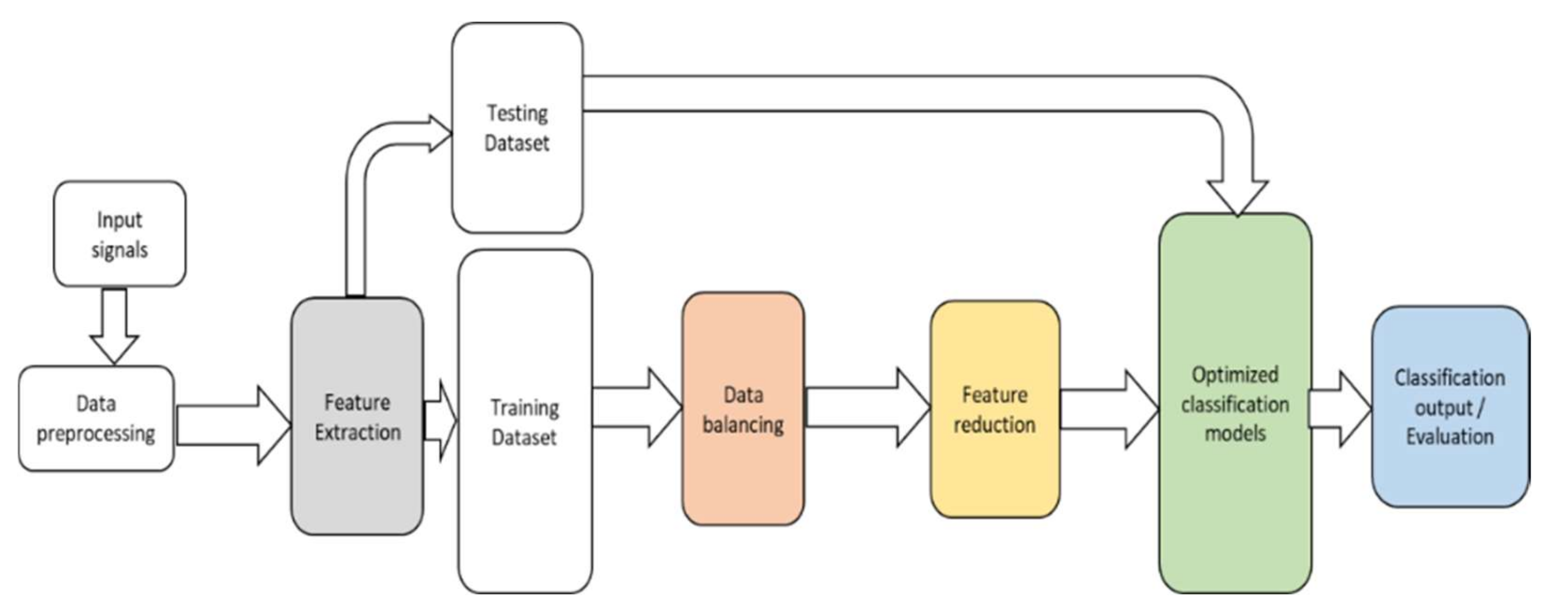
- Machine learning techniques: Many researchers proposed artificial intelligence techniques that utilize machine learning (ML) in power system protection for fault detection, classification, and localization. The implementation of machine learning for power system fault diagnosis was reviewed in [10,22,23]. The ultimate advantages of these techniques are the accuracy, self-adaptiveness, and robustness to parameter variations [24]. Existing ML techniques comprise the following stages: preprocessing, feature extraction, feature reduction, classification, and performance evaluation. For our focus, transmission line fault detection, classification, and localization using machine learning techniques are reviewed in this article.
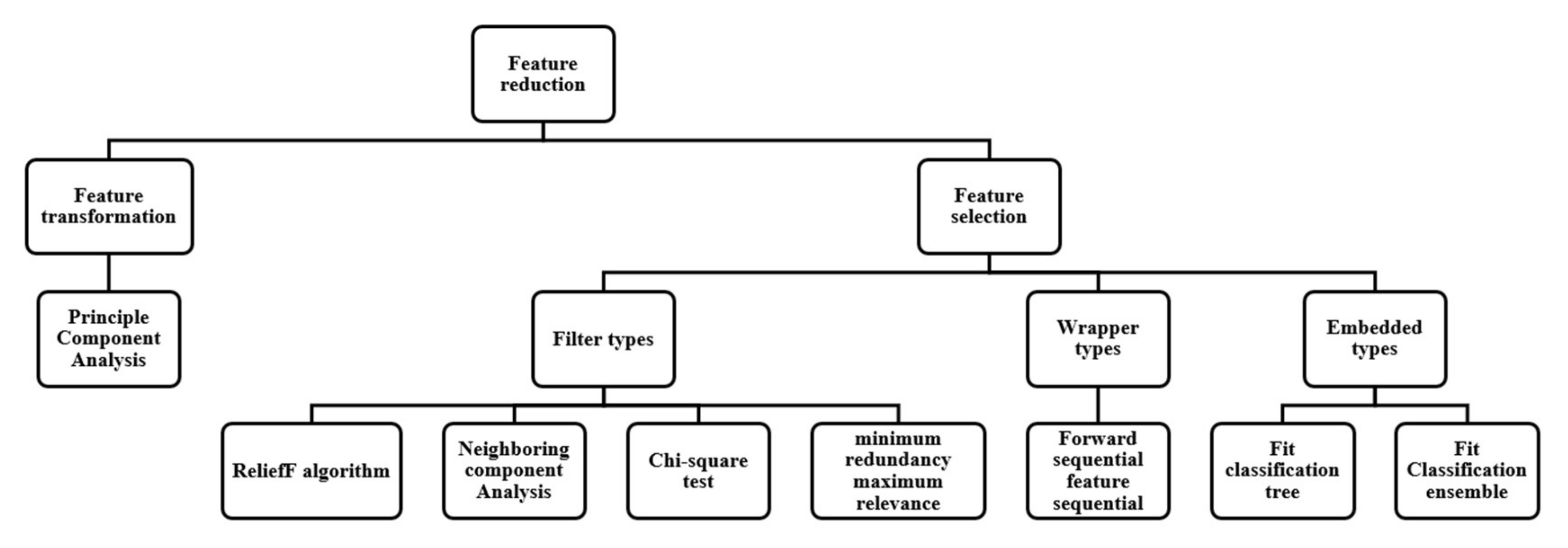
- Few feature selection techniques were investigated to find the optimum feature subset. In most cases, filter types (Information gain, Mutual information, etc.), wrapper type (forward feature selection), and feature transformation (PCA) were considered, but none of the researchers considered the embedded-type feature selection techniques.
- The issue of data imbalance was not highlighted, and the impact on the detection/classification performance was not investigated.
- Insufficient research addresses the problem of fault detection and classification in the presence of inverter-based renewables.
- The classification accuracy was dominantly used as the only metric to evaluate the classifier’s performance, which could not be sufficient if the data was unbalanced.
- The classifiers’ hyperparameters tuning with optimization algorithms were not considered.
- to conduct a comprehensive study of ML-based transmission line fault classification involving many features extracted from different domains (time, frequency, and time–frequency), different feature selection/transformation algorithms, and many widely used ML-based classification models;
- to investigate the critical problem of data imbalance as faults are relatively rare events in power systems. The class unbalancing is addressed using the synthetic minority class oversampling technique (SMOTE) and by
- optimization of the classifiers’ hyperparameters.
2. Methodology
2.1. System Study and Data Preparation
2.2. Feature Extraction
2.3. Data Balancing
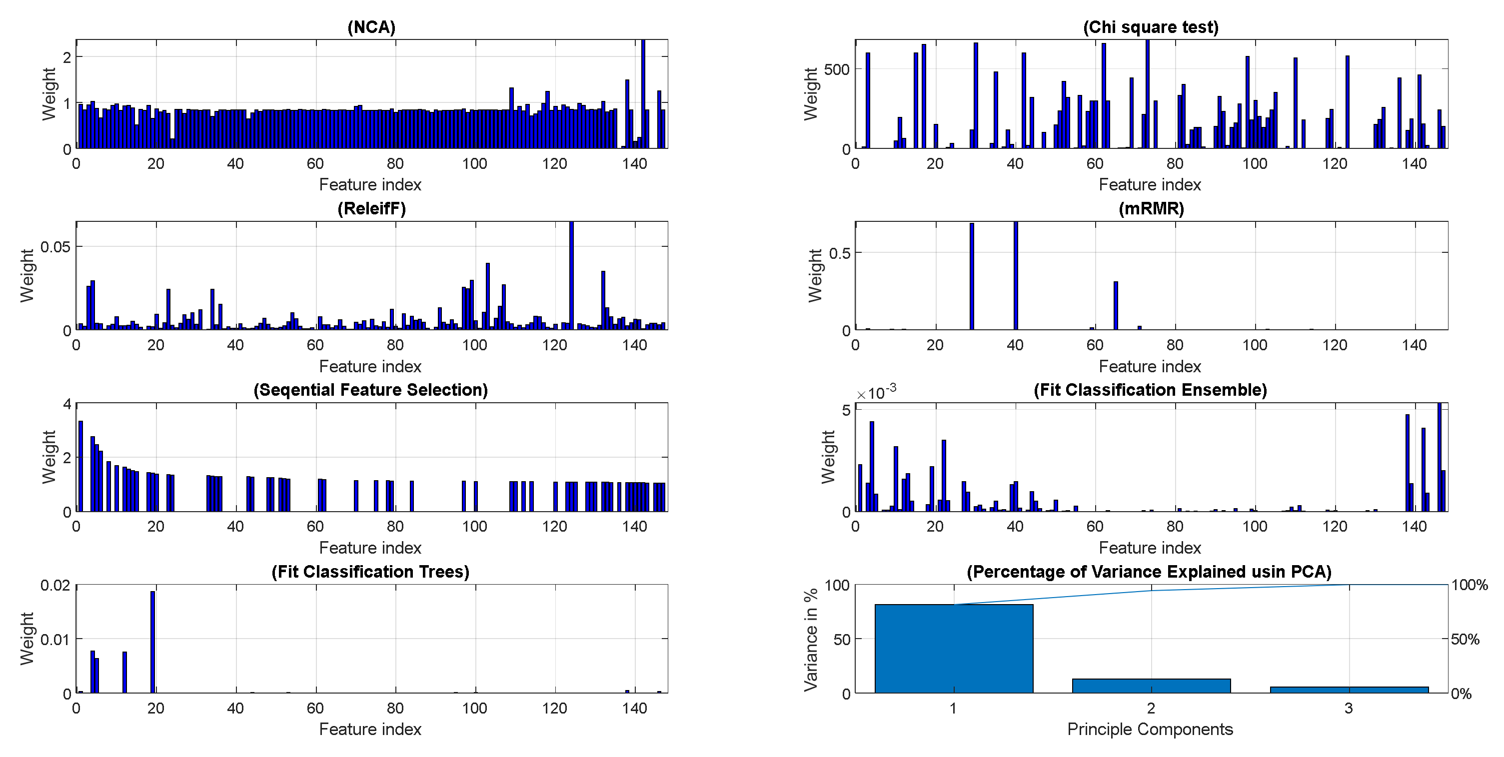
2.4. Feature Reduction
2.5. Classification Models
2.6. Evaluation Metrics
- Accuracy is the ratio of the number of correct predictions (fault and non-fault events) to the total number of input samples in the test dataset.
- Sensitivity is the percentage of true positives (non-fault events) that are correctly identified by the classifier.
- Specificity is the percentage of true negatives (fault events) that are correctly identified by the classifier.
- Precision indicates the percentage of instances the classifier detected as positives compared to the total positive instances.
3. Results and Discussion of Results
3.1. Performance of Fault Detection Model
3.1.1. Performance of Balanced versus Unbalanced Datasets
- The classification performance of the four proposed classifiers was generally high. The Bag Ensemble and decision trees achieved better performance than k-NN and SVM.
- Balancing the dataset improved the specificity and sensitivity of the SVM and k-NN classifiers.
- The training time for the balanced dataset increased dramatically as the number of observations of the minority class (fault events) increased. In addition, the training time for the classifiers with more tuned parameters was higher, as in the case of tuning the k-NN and Ensemble.
3.1.2. Performance of Reduced Dataset
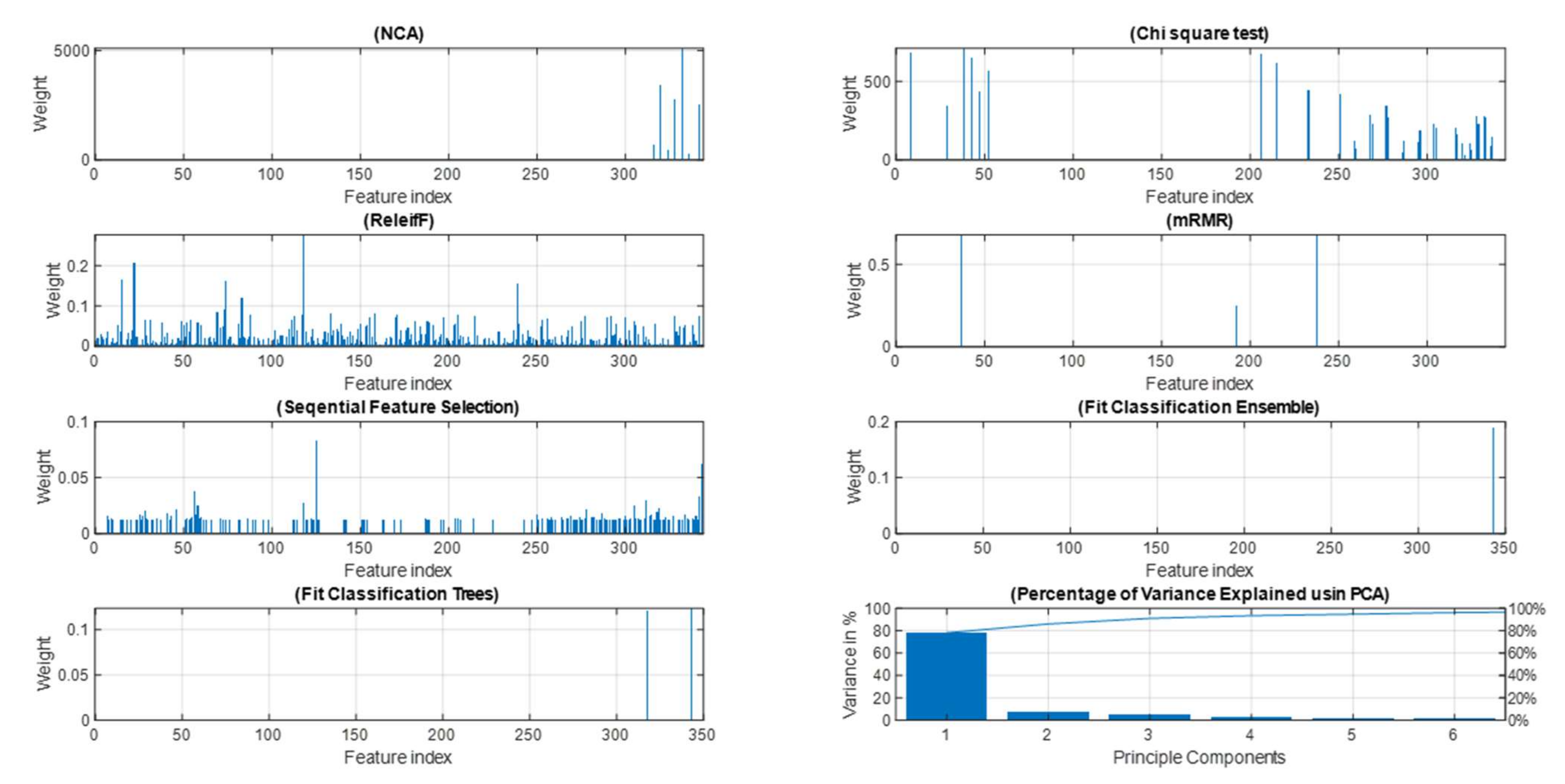
- With only 163 features selected using the sequential forward feature selection method, the classification performance was the highest using the Bag ensemble classifier. However, the training time was high.
- In the embedded-type feature selection methods (Fit trees and Fit Ensemble), single and two features were selected, respectively, with remarkable classification performance. The training time was low compared with others because of the small dimension of the training data.
- The mRMR feature selection algorithm with the k-NN classifier achieved the lowest performance.
- The chi-square test selected only 34 features, but the training time to tune the hyperparameters of the k-NN classifier was the highest. Its performance was quite good but less than NCA and ReleifF techniques.
- The Ensemble and DT classifiers were the best classifiers with most types of feature selection except for mRMR algorithm, where the k-NN was the best performer.
- The SVM with Gaussian kernel gave relatively poor results with all feature reduction algorithms.
- The PCA with GentleBoost Ensemble classifier performed well using 95% of the variance explained, but the training time was considerably high.
3.2. Performance of Fault Classification Model
3.2.1. Performance with a Complete Set of Features
3.2.2. Performance of Reduced Dataset
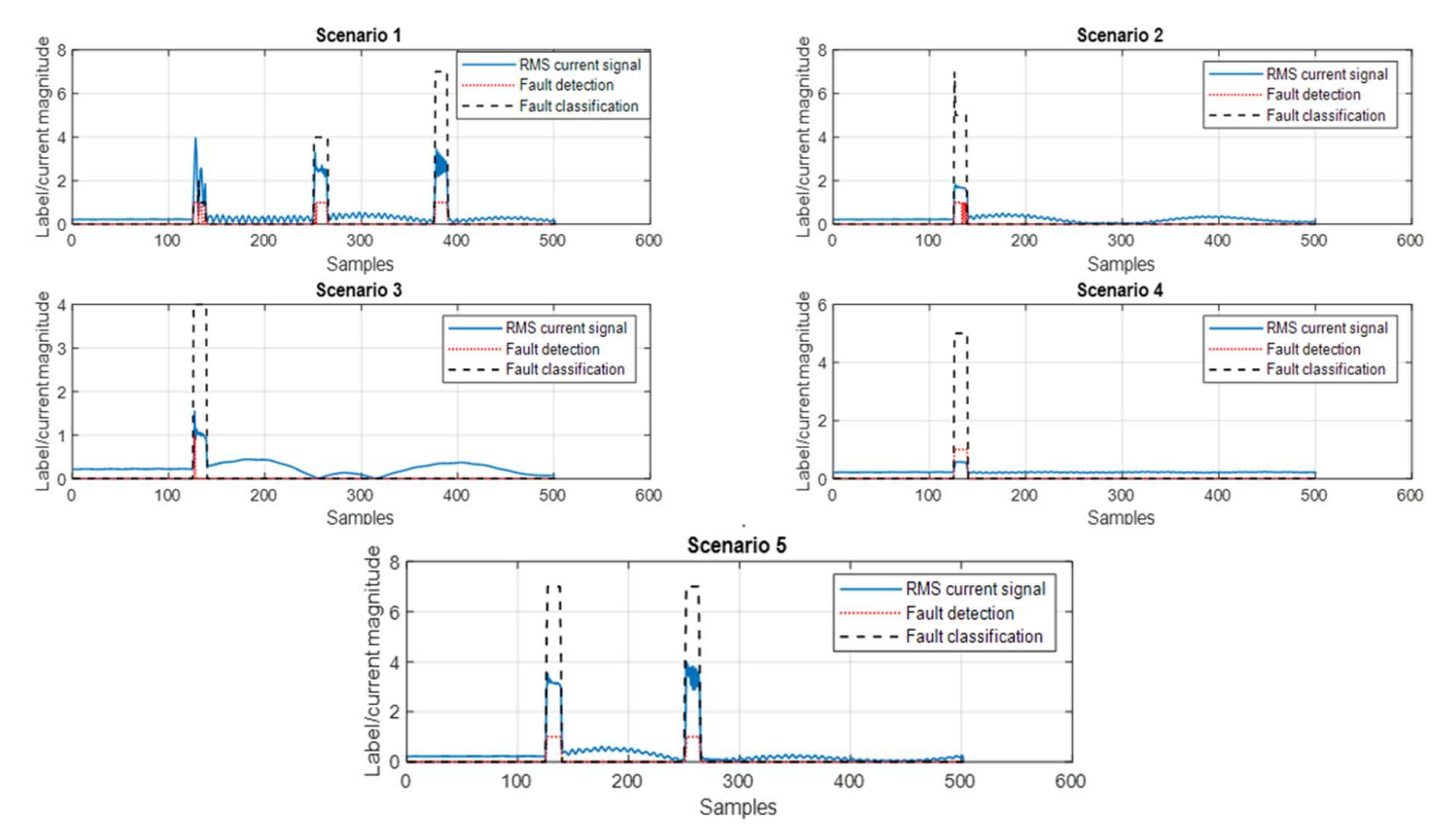
3.3. Performance Evaluation Using New Fault Scenarios
- Scenario 1: Three cascaded in-zone faults at 70% of the protected line (Line 1–2) from the measurement point were simulated. The first fault was A-G at 1.0 s, the second was A-B at 2.0 s, and the third was A-B-C fault at 3.0 s. The fault duration was 0.1 s. The generation connected to Bus 02 was G10 and PV plant. The faults were correctly detected and classified except for A-G fault, where the classifier was confused between class 1 (A-G) & class 2 (B-G).
- Scenario 2: Out of zone fault in the line (1–39) at 50%. The fault was A-B-C fault incepted at 1.0 s for 100 ms. The generation connected to Bus 02 was G10 and Windfarm. The fault was detected. The fault type was initially detected as A-B-C fault at the inception of the fault, and then, during the fault, it was classified as A-C fault. Out-of-zone detection could be mitigated by introducing fault detection with ML for each line in the system.
- Scenario 3: Out of zone fault in the line (2–25) at 50%. The fault was A-B fault incepted at 1.0 s for 100 ms. The generation connected to Bus 02 was G10 and Windfarm. The fault was detected and classified accurately, although the fault was not located at the protected line. Similar to Scenario 2, out-of-zone detection could be mitigated by introducing fault detection with ML for each line in the system.
- Scenario 4: High impedance fault with fault resistance of 200 ohms was incepted at 70% of the line (01–02). The fault was A-B-C fault. The generation connected to Bus 02 was G10 and PV Plant. The fault was correctly detected.
- Scenario 5: Fault during power swing was created at 2.0 s, and the power swing occurred due to fault clearance that happened at 1.0 s. Both faults were A-B-C faults created at 50% of the line (01–02). The generation connected to Bus 02 was G10 and PV Plant. The faults were correctly detected and classified.
3.4. Comparative Analysis of Different Methods in the Literature
4. Conclusions
- The results showed that the data balancing using SMOTE improved the specificity and sensitivity metrics however the training time increased dramatically.
- Each proposed feature-reduction method developed a different selected subset of features and resulted in different classification performance.
- The Ensemble and DT classifiers performed better than others in most types of feature selection.
- The forward feature selection technique with the Bag ensemble classifier improved the classification metrics to 100% for fault detection using 163 features.
- The Adaboost ensemble classifier had the highest accuracy compared with other classifiers with 99.4% for fault type classification.
- The prediction capability for fault detection and classification was high using the complete set of features when tested with new test cases.
- Compared with other methodologies from the literature, the implemented approach resulted in high detection and classification capability considering the integration of IBGs.
Author Contributions
Funding
Institutional Review Board Statement
Informed Consent Statement
Data Availability Statement
Acknowledgments
Conflicts of Interest
Appendix A
Features Description
Appendix B
Experimental Settings
| 39-Bus Power System | As Detailed in [34]. |
| PV inverter | 10 kVA per inverter, local controller: constant Q, Short circuit model: Dynamic voltage support, Sub-transient short circuit: 1.21 kVA, R to X” ratio: 0.1, K Factor: 2, Max. current: 1.1 pu, Td” = 0.03 s, Td’ = 1.2 s |
| Wind Turbine | 2 MVA, 1.0 power factor, local controller: constant Q, Short circuit model: Dynamic voltage support, Sub-transient short circuit: 2.39 MVA, R to X” ratio: 0.1, K Factor: 2, Max. current: 1.1 pu, Td” = 0.03 s, Td’ = 1.2 s |
| SPECTROGRAM | Window size: 16 samples, overlapping: 16 samples |
| SMOTE | Number of nearest neighbors: 5, Oversampling rate: 450%, Random seeds: 100 |
| Optimizer settings | Optimizer: Bayesian Optimization, Acquisition function: Expected improvement per second plus, Iterations: 10 |
| Sequential feature selection algorithm | Criterion function: Residual Sum of Squares, Validation method: 5-fold cross-validation |
| ReliefF algorithm | Number of nearest neighbors: 5 |
| PCA | Percentage of variance explained: 95% |
| Classifier-1 datasets (Fault Detection) |
|
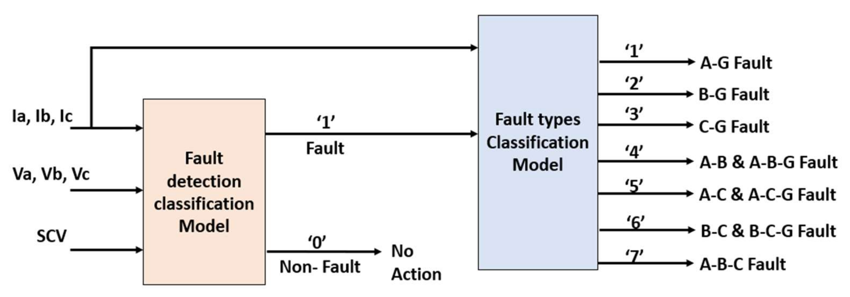
| Classifier-2 datasets (Fault Classification) | Labels: ‘1’: A_G fault, ‘2’: B-G fault, ‘3’: C-G fault, ‘4’: A-B & A-B-G fault, ‘5’: A-C & A-C-G fault, ‘6’: B-C & B-C-G fault, and ‘7’: A-B-C fault Training Dataset: Number of observations: 278 (A-Gfault), 277 (B-G fault), 263 (C-G fault), 521 (A-B & A-B-G fault), 540 (A-C & A-C-G fault), 524 (B-C & B-C-G fault), and 258 (B-C & B-C-G fault) Testing Dataset: Number of observations: 104 (A-G fault), 104 (B-G fault), 118 (C-G fault), 238 (A-B & A-B-G fault), 219 (A-C & A-C-G fault), 235 (B-C & B-C-G fault), and 122 (B-C & B-C-G fault) Features: 147 extracted features from only current signals (Ia, Ib, and Ic) as defined in Table 2. |
References
- IEEE Power & Energy Society. PES-TR81—Protection Challenges and Practices for Interconnecting Inverter Based Resources to Utility Transmission Systems. 2020. Available online: https://resourcecenter.ieee-pes.org/technical-publications/technical-reports/PES_TP_TR81_PSRC_WGC32_071520.html (accessed on 2 May 2020).
- Liu, S.; Bi, T.; Liu, Y. Theoretical analysis on the short-circuit current of inverter-interfaced renewable energy generators with fault-ride-through capability. Sustainability 2017, 10, 44. [Google Scholar] [CrossRef] [Green Version]
- Mahamedi, B.; Fletcher, J.E. Trends in the protection of inverter-based microgrids. IET Gener. Transm. Distrib. 2019, 13, 4511–4522. [Google Scholar] [CrossRef]
- Haj-Ahmed, M.A.; Feilat, E.A.; Khasawneh, H.J.; Abdelhadi, A.F.; Awwad, A. Comprehensive Protection Schemes for Different Types of Wind Generators. IEEE Trans. Ind. Appl. 2018, 54, 2051–2058. [Google Scholar] [CrossRef]
- North Americam Electric Reliability Corporation (NERC). Short-circuit modeling and system strength. In White Papar; North Americam Electric Reliability Corporation: Atlanta, GA, USA, 2018. [Google Scholar]
- IEEE Power and Energy Society. IEEE Std 2800; IEEE Standard for Interconnection and Interoperability of Inverter-Based Resources (IBRs) Interconnecting with Associated Transmission Electric Power Systems. IEEE: Manhattan, NY, USA, 2022.
- Liang, Z.; Lin, X.; Kang, Y.; Gao, B.; Lei, H. Short Circuit Current Characteristics Analysis and Improved Current Limiting Strategy for Three-phase Three-leg Inverter under Asymmetric Short Circuit Fault. IEEE Trans. Power Electron. 2018, 33, 7214–7228. [Google Scholar] [CrossRef]
- IEEE/NERC. Task force on Short-Circuit and System Performance Impact of Inverter Based Generation: Impact of Inverter Based Generation on Bulk Power System Dynamics and Short-Circuit Performance; Technical report; IEEE: Manhattan, NY, USA, 2018. [Google Scholar]
- Usama, M.; Mokhlis, H.; Moghavvemi, M.; Mansor, N.N.; Alotaibi, M.A.; Muhammad, M.A.; Bajwa, A.A. A Comprehensive Review on Protection Strategies to Mitigate the Impact of Renewable Energy Sources on Interconnected Distribution Networks. IEEE Access 2021, 9, 35740–35765. [Google Scholar] [CrossRef]
- Senarathna, S.; Hemapala, K.T.M.U. Review of adaptive protection methods for microgrids. AIMS Energy 2019, 7, 557–578. [Google Scholar] [CrossRef]
- Kaur, G.; Prakash, A.; Rao, K.U. A critical review of Microgrid adaptive protection techniques with distributed generation. Renew. Energy Focus 2021, 39, 99–109. [Google Scholar] [CrossRef]
- Adly, A.R.; Aleem, S.H.E.A.; Algabalawy, M.A.; Jurado, F.; Ali, Z.M. A novel protection scheme for multi-terminal transmission lines based on wavelet transform. Electr. Power Syst. Res. 2020, 183, 106286. [Google Scholar] [CrossRef]
- Sakis, G.J.C.; Meliopoulos, A.P. Setting-less Protection. In Proceedings of the 2013 46th Hawaii International Conference on System Sciences, Wailea, HI, USA, 7–10 January 2013. [Google Scholar]
- Okedu, K.E. Enhancing DFIG wind turbine during three-phase fault using parallel interleaved converters and dynamic resistor. IET Renew. Power Gener. 2016, 10, 1211–1219. [Google Scholar] [CrossRef]
- Chen, L.; Li, G.; Chen, H.; Tao, Y.; Tian, X.; Liu, X.; Xu, Y.; Ren, L.; Tang, Y. Combined Use of a Resistive SFCL and DC-link Regulation of a SMES for FRT Enhancement of a DFIG Wind Turbine Under Different Faults. IEEE Trans. Appl. Supercond. 2019, 29, 1–8. [Google Scholar] [CrossRef]
- Papaspilotopoulos, N.H.V.; Korres, G. An Adaptive Protection Infrastructure for Modern Distribution Grids with Distributed Generation. Cigre Sci. Eng. 2016, 7, 125–132. [Google Scholar]
- Hossain, M.; Ali, M.H. Transient stability improvement of doubly fed induction generator based variable speed wind generator using DC resistive fault current limiter. IET Renew. Power Gener. 2016, 10, 150–157. [Google Scholar] [CrossRef]
- Alam, S.; Abido, M.A.Y.; El-Amin, I. Fault Current Limiters in Power Systems: A Comprehensive Review. Energies 2018, 11, 1025. [Google Scholar] [CrossRef] [Green Version]
- Wang, K.; Guo, M.; Dai, C.; Li, Z. Information-decision searching algorithm: Theory and applications for solving engineering optimization problems. Inf. Sci. 2022, 607, 1465–1531. [Google Scholar] [CrossRef]
- El-Naily, N.; Saad, S.M.; Elhaffar, A.; Zarour, E.; Alasali, F. Innovative Adaptive Protection Approach to Maximize the Security and Performance of Phase/Earth Overcurrent Relay for Microgrid Considering Earth Fault Scenarios. Electr. Power Syst. Res. 2022, 206, 107844. [Google Scholar] [CrossRef]
- Chopard, B.; Tomassini, M. Performance and limitations of metaheuristics. In An Introduction to Metaheuristics for Optimization; Natural Computing Series; Springer: Cham, Switzerland, 2018; pp. 191–203. [Google Scholar]
- Rahman Fahim, S.; Sarker, S.K.; Muyeen, S.M.; Sheikh, M.; Islam, R.; Das, S.K. Microgrid Fault Detection and Classification: Machine Learning Based Approach, Comparison, and Reviews. Energies 2020, 13, 3460. [Google Scholar] [CrossRef]
- Pérez-Ortiz, M.; Jiménez-Fernández, S.; Gutiérrez, P.A.; Alexandre, E.; Hervás-Martínez, C.; Salcedo-Sanz, S. A Review of Classification Problems and Algorithms in Renewable Energy Applications. Energies 2016, 9, 607. [Google Scholar] [CrossRef]
- Ray, P.; Mishra, D.P. Support vector machine based fault classification and location of a long transmission line. Eng. Sci. Technol. Int. J. 2016, 19, 1368–1380. [Google Scholar] [CrossRef] [Green Version]
- Swetapadma, A.; Yadav, A.; Abdelaziz, A.Y. Intelligent schemes for fault classification in mutually coupled series-compensated parallel transmission lines. Neural Comput. Appl. 2020, 32, 6939–6956. [Google Scholar] [CrossRef]
- Wasnik, P.P.; Phadkule, N.J.; Thakur, K.D. Fault Detection and Classification in Transmission Line by using KNN and DT Technique. Int. Res. J. Eng. Technol. 2020, 7, 335–340. [Google Scholar]
- Patil, D.; Naidu, O.D.; Yalla, P.; Hida, S. An Ensemble Machine Learning Based Fault Classification Method for Faults During Power Swing. In Proceedings of the 2019 IEEE PES Innovative Smart Grid Technologies Asia, ISGT 2019, Chengdu, China, 21–24 May 2019; pp. 4225–4230. [Google Scholar] [CrossRef]
- Lwin, M.; Min, K.W.; Padullaparti, H.V.; Santoso, S. Symmetrical fault detection during power swings: An interpretable supervised learning approach. In Proceedings of the IEEE Power and Energy Society General Meeting, Portland, OR, USA, 5–9 August 2018; pp. 1–5. [Google Scholar] [CrossRef]
- Mukherjee, A.; Kundu, P.K.; Das, A. Application of Principal Component Analysis for Fault Classification in Transmission Line with Ratio-Based Method and Probabilistic Neural Network: A Comparative Analysis. J. Inst. Eng. India Ser. B 2020, 101, 321–333. [Google Scholar] [CrossRef]
- Mukherjee, A.; Kundu, P.K.; Das, A. Transmission Line Fault Location Using PCA-Based Best-Fit Curve Analysis. J. Inst. Eng. India Ser. B 2021, 102, 339–350. [Google Scholar] [CrossRef]
- Akmaz, D.; Mamiş, M.S.; Arkan, M.; Tağluk, M.E. Transmission line fault location using traveling wave frequencies and extreme learning machine. Electr. Power Syst. Res. 2018, 155, 106034. [Google Scholar] [CrossRef]
- Sharma, S.K. GA-GNN (Genetic Algorithm-Generalized Neural Network)-Based Fault Classification System for Three-Phase Transmission System. J. Inst. Eng. India Ser. B 2019, 100, 435–445. [Google Scholar] [CrossRef]
- Patel, B. A new FDOST entropy based intelligent digital relaying for detection, classification and localization of faults on the hybrid transmission line. Electr. Power Syst. Res. 2018, 157, 39–47. [Google Scholar] [CrossRef]
- DIgSILENT Power Factory. 39 Bus New England System; Power Factory: Gomaringen, Germany, 2015; pp. 1–16. [Google Scholar]
- Lammert, G.; Ospina, L.D.P.; Pourbeik, P.; Fetzer, D.; Braun, M. Implementation and validation of WECC generic photovoltaic system models in DIgSILENT PowerFactory. In Proceedings of the IEEE Power and Energy Society General Meeting, Boston, MA, USA, 17–21 July 2016; pp. 3–7. [Google Scholar] [CrossRef]
- Hiskens, I.A. Dynamics of Type-3 Wind Turbine Generator Models. IEEE Trans. Power Syst. 2012, 27, 465–474. [Google Scholar] [CrossRef] [Green Version]
- Benmouyal, G.H.D.T. Zero-setting power-swing blocking protection. In Proceedings of the 3rd IEE International Conference on Reliability of Transmission and Distribution Networks (RTDN 2005), London, UK, 15–17 February 2005; pp. 249–254. [Google Scholar] [CrossRef] [Green Version]
- Jarrahi, M.A.; Samet, H.; Ghanbari, T. Fast Current-Only Based Fault Detection Method in Transmission Line. IEEE Syst. J. 2019, 13, 1725–1736. [Google Scholar] [CrossRef]
- Chiradeja, P.; Ngaopitakkul, A. Classification of Lightning and Faults in Transmission Line Systems Using Discrete Wavelet Transform. Math. Probl. Eng. 2018, 2018, 1847968. [Google Scholar] [CrossRef]
- Nandi, H.A.K. Condition Monitoring with Vibration Signals: Compressive Sampling and Learning Algorithms for Rotating Machines; JohnWiley & Sons: Hoboken, NJ, USA, 2019; Volume 53. [Google Scholar]
- Ramos-Aguilar, R.; Olvera-López, J.A.; Olmos-Pineda, I.; Sánchez-Urrieta, S. Feature extraction from EEG spectrograms for epileptic seizure detection. Pattern Recognit. Lett. 2020, 133, 202–209. [Google Scholar] [CrossRef]
- Aliyu, I.; Lim, C.G. Selection of optimal wavelet features for epileptic EEG signal classification with LSTM. Neural Comput. Appl. 2021, 1–21. [Google Scholar] [CrossRef]
- Taheri, B.; Salehimehr, S.; Razavi, F.; Parpaei, M. Detection of power swing and fault occurring simultaneously with power swing using instantaneous frequency. Energy Syst. 2020, 11, 491–514. [Google Scholar] [CrossRef]
- Kłosowski, G.; Rymarczyk, T.; Wójcik, D.; Skowron, S.; Cieplak, T.; Adamkiewicz, P. The Use of Time-Frequency Moments as Inputs of LSTM Network for ECG Signal Classification. Electronics 2020, 9, 1452. [Google Scholar] [CrossRef]
- Phinyomark, A.; Thongpanja, S.; Hu, H.; Phukpattaranont, P.; Limsakul, C. The Usefulness of Mean and Median Frequencies in Electromyography Analysis. In Computational Intelligence in Electromyography Analysis—A Perspective on Current Applications and Future Challenges; IntechOpen: London, UK, 2012; pp. 195–220. [Google Scholar]
- Remeseiro, B.; Bolon-Canedo, V. A review of feature selection methods in medical applications. Comput. Biol. Med. 2019, 112, 103375. [Google Scholar] [CrossRef] [PubMed]
- Niyas, M.; Sunitha, K. Identification and classification of fault during power swing using decision tree approach. In Proceedings of the 2017 IEEE International Conference on Signal Processing, Informatics, Communication and Energy Systems, SPICES 2017, Kollam, India, 8–10 August 2017; pp. 1–6. [Google Scholar] [CrossRef]
- Yang, C.; Yang, J.; Ma, J. Adaptive Kernel Parameters. Int. J. Comput. Intell. Syst. 2020, 13, 212–222. [Google Scholar] [CrossRef] [Green Version]
- Blagus, R.; Lusa, L. SMOTE for high-dimensional class-imbalanced data. BMC Bioinform. 2013, 14, 106. [Google Scholar] [CrossRef] [PubMed] [Green Version]
- Yang, L.; Shami, A. On hyperparameter optimization of machine learning algorithms: Theory and practice. Neurocomputing 2020, 415, 295–316. [Google Scholar] [CrossRef]
- Swamynathan, M. Mastering Machine Learning with Python in Six Steps: A Practical Implementation Guide to Predictive Data Analytics Using Python, 2nd ed.; Apress: New York, NY, USA, 2019; Volume 126. [Google Scholar]
- Mathworks, C. Statistics and Machine Learning Toolbox TM User’s Guide R 2016 b. 2016. Available online: https://www.mathworks.com/products/statistics.html (accessed on 25 May 2022).
- Brownlee, J. Imbalanced Classification with Python: Better Metrics, Balance Skewed Classes, Cost-Sensitive Learning, V1.3; Machine Learning Mastery. 2020. Available online: https://www.scribd.com/document/517979097/Imbalanced-Classification-With-Python-by-Jason-Brownlee-Z-lib-org (accessed on 25 May 2022).
- Gadekallu, T.R.; Khare, N.; Bhattacharya, S.; Singh, S.; Maddikunta, P.K.R.; Ra, I.-H.; Alazab, M. Early Detection of Diabetic Retinopathy Using PCA-Firefly Based Deep Learning Model. Electronics 2020, 9, 274. [Google Scholar] [CrossRef] [Green Version]


| Fault Cases | Generator Type Connected to Bus 2 | Fault Location (%) | Fault Impedance (ohms) | Fault Types |
|---|---|---|---|---|
| Cases from 1 to 10 | G10, PV, WF *, G10 & PV, and G10 & WF | 10 | Zero | A-G, B-G, C-G, A-B, A-C, B-C, A-B-G, A-C-G, B-C-G and A-B-C |
| Cases from 11 to 20 | 50 | Zero | ||
| Cases from 21 to 30 | 90 | Zero | ||
| Cases from 31 to 40 | 10 | 100 | ||
| Cases from 41 to 50 | 50 | 100 | ||
| Cases from 51 to 60 | 90 | 100 |
| Domain | Features | Number of Features for Each Signal |
|---|---|---|
| Time | Statistical features of original signals [40] | 9 |
| Statistical features of first-order difference of the original signals [40] | 9 | |
| Time-frequency | Statistical features of spectrogram [41] | 9 |
| Statistical features of wavelet decomposition of first and second detail coefficients [42] | 18 | |
| Estimated instantaneous frequency [43] | 1 | |
| Frequency | Spectral entropy [44] | 1 |
| Mean and median frequency [45] | 2 |
| Model | Hyper-Parameters | Search Options | Remarks |
|---|---|---|---|
| Optimizable Tree | Maximum number of splits | Search among integers log-scaled in the range [1, max(2, n − 1)] | Specify the maximum number of splits or branch points to control the depth of the tree. |
| Split criterion | Gini’s diversity index, Towing rule, and Maximum deviance reduction | This is to decide when to split the nodes. | |
| Optimizable GSVM | Box constraint level | Range [0.001, 1000] | This is to keep the allowable values of the Lagrange multipliers in a box. |
| Multiclass method Standardize data | Search between true and false | If predictors have widely different scales, standardizing can improve the fit. | |
| Optimizable k-NN | Number of neighbors | Search among integers log-scaled in the range [1, max (2,n − 1)] | A fine kNN uses fewer neighbors, and a coarse kNN uses higher neighbors. |
| Distance metric | Euclidean, City block, Chebyshev, Minkowski (cubic), Mahalanobis, Cosine, Correlation, Spearman, Hamming, Jaccard | These are metrics to determine the distance to points. | |
| Distance weight | Searches among Equal, Inverse, and Squared inverse. | Specify the distance weighting function. | |
| Standardized data | Search between true and false | Standardizing the data can improve the fit if predictors have widely different scales. | |
| Optimizable Ensemble | Ensemble method | Search among AdaBoost, RUSBoost, LogitBoost, GentleBoost, and Bag | |
| Maximum number of splits | Search among integers log-scaled in the range [1, max(2, n − 1)] | Specify the maximum number of splits or branch points to control the depth of the tree. | |
| Number of learners | Search among integers log-scaled in the range [10, 500] | Many learners can produce high accuracy but can be time-consuming to fit | |
| Learning rate | Search among real values log-scaled in the range [0.001, 1] | If the learning rate is set to less than 1, the Ensemble requires more learning iterations but often achieves better accuracy. |
| Metric | Defined as | Confusion Matrix | |||
|---|---|---|---|---|---|
| Accuracy | (TP + TN)/(TP + FN + FP + TN) * | Predicted Class | |||
| Sensitivity | TP/(TP + FN) | Class 0 | Class 1 | ||
| Specificity | TN/(TN + FP) | Actual Class | Class 0 | TP | FN |
| Precision | TP/(TP + FP) | Class 1 | FP | TN | |
| Classifier | Unbalanced Dataset | Balanced Dataset | ||
|---|---|---|---|---|
| Hyperparameters | Training Time (s) | Hyperparameters | Training Time (s) | |
| DT | Maximum number of splits: 428, Split criterion: Maximum deviance reduction | 188 | Maximum number of splits: 34,833, Split criterion: Maximum deviance reduction | 227 |
| SVM | Box constraint level: 47.0829, Standardize data: false | 2058 | Box constraint level: 995.6227, Standardize data: false | 21,324 |
| K-NN | Number of neighbors: 1, Distance weight: Inverse, Standardize data: true | 5390 | Number of neighbors: 1, Distance metric: Euclidian, Distance weight: Equal, Standardize data: true | 15,187 |
| Ensemble | Ensemble method: Bag, Maximum number of splits: 30,209, number of learners: 13, number of predictors to sample: 60 | 819 | Ensemble method: Bag, Maximum number of splits: 16, number of learners: 228, number of predictors to sample: 145 | 17,680 |
| Feature Reduction Method | Best Classifier | Number of Selected Features | Accuracy (%) | Sensitivity (%) | Specificity (%) | Precision (%) | Hyperparameters | Training Time (s) |
|---|---|---|---|---|---|---|---|---|
| NCA | Ensemble | 8 | 99.98 | 99.98 | 100.00 | 100.00 | Ensemble method: GentleBoost, Maximum number of splits: 283, number of learners: 274, Learning rate: 0.007819 | 804 |
| Chi-square test | Ensemble | 34 | 99.55 | 99.75 | 96.72 | 99.77 | Ensemble method: AdaBoost, Maximum number of splits: 1087, number of learners: 136, Learning rate: 0.66932 | 14,327 |
| ReliefF | DT | 122 | 100.00 | 100.00 | 99.93 | 99.99 | Maximum number of splits: 86,022, Split criterion: Gini’s diversity index | 104 |
| mRMR | KNN | 3 | 91.02 | 91.51 | 84.21 | 98.77 | Number of neighbors: 28, Distance metric: Euclidean, Distance weight: Equal | 552 |
| Forward Sequential feature | Ensemble | 163 | 100.00 | 100.00 | 100.00 | 100.00 | Ensemble method: Bag, Maximum number of splits: 15,701, number of learners: 17, number of predictors to sample: 39 | 1223 |
| Fit classification ensemble | Ensemble | 1 | 99.63 | 99.61 | 99.86 | 99.99 | Ensemble method: RUSBoost, Maximum number of splits: 1, number of learners: 10, Learning rate: 0.0073088 | 146 |
| Fit classification trees | DT | 2 | 99.99 | 100.00 | 99.78 | 99.98 | Maximum number of splits: 49, Split criterion: Maximum deviance reduction | 31 |
| PCA | Ensemble | 6 components | 98.92 | 99.13 | 95.94 | 99.71 | Ensemble method: GentleBoost, Maximum number of splits: 57, number of learners: 210 | 12,037 |
| Feature Reduction Method | Best Classifier | Number of Selected Features | Accuracy (%) | Hyperparameters | Training Time (s) |
|---|---|---|---|---|---|
| NCA | DT | 103 | 98.5 | Maximum number of splits: 2643, Split criterion: Maximum deviance reduction | 23 |
| Chi-square test | Ensemble | 87 | 97.5 | Ensemble method: AdaBoost, Maximum number of splits: 14, number of learners: 24, Learning rate: 0.0023388 | 145 |
| ReliefF | Ensemble | 41 | 98.2 | Ensemble method: AdaBoost, Maximum number of splits: 7, number of learners: 449, Learning rate: 0.99393 | 324 |
| mRMR | Ensemble | 5 | 70.9 | Ensemble method: Bag, Maximum number of splits: 618, number of learners: 245, number of predictors to sample: 2 | 236 |
| Forward Sequential feature | Ensemble | 57 | 98.8 | Ensemble method: RUSBoost, Maximum number of splits: 112, number of learners: 11, Learning rate: 0.73117 | 133 |
| Fit classification ensemble | Ensemble | 24 | 99.0 | Ensemble method: Bag, Maximum number of splits: 36, number of learners: 95, number of predictors to sample: 8 | 148 |
| Fit classification trees | Ensemble | 14 | 98.9 | Ensemble method: Bag, Maximum number of splits: 220, number of learners: 12, number of predictors to sample: 5 | 68 |
| PCA | Ensemble | 3 components | 74.6 | Ensemble method: Bag, Maximum number of splits: 2619, number of learners: 473, number of predictors to sample: 3 | 202 |
| Reference | Objective | Methodology | IBG Consideration | Classifiers | Performance Metrics | Classification Results |
|---|---|---|---|---|---|---|
| [25] | Fault detection and classification for mutually coupled transmission lines | Discrete Wavelet Transformation was used to extract the features from three-phase currents. Twenty-one classes were considered for phase fault identification and four classes for ground fault identification. The data balancing was not considered, and no feature reduction technique was used. | No | ANN, k-NN, and DT. | Accuracy | Accuracy = 100% (ANN) |
| [26] | Fault detection and classification | Discrete Wavelet Transformation was used to extract the features from three-phase currents and voltages. Twelve classes were considered for normal events and different fault types. The data balancing was not reported, and no feature reduction technique was used. | No | k-NN and DT | Accuracy | Accuracy = 100% (DT) |
| [24] | Fault classification and localization | Wavelet packet transformation was used to extract the features from three-phase voltages and currents. The data was reported balanced, and the Forward feature selection algorithm was used to reduce the number of features. Ten classes were introduced for normal conditions and fault events with different types of faults. | No | SVM | Accuracy for classification, and absolute error for fault localization | Accuracy = 99.21% absolute error < 0.21% |
| [28] | Classification of symmetrical faults during power swing | Changes in current magnitude, voltage magnitude, current angle, voltage angle, active power, reactive power, apparent resistance, and reactance were considered the features of Voltage and current magnitude and angle, active and reactive power, and apparent impedance signals. Data balancing was not reported, and the Mutual information technique was used for feature selection. Two classes were considered for fault and swing events. | No | k-NN, DT, k-NN, Boost ensemble, SVM, and Random Forest | Accuracy, and receiver operating characteristic (ROC) | Accuracy = 98.2% (Boost ensemble) ROC = 1.0 |
| [29] | Fault detection and classification | Principle component scores of three-phase current signals were used as features. The dataset was created balanced. Eleven classes were used, one for non-fault events and ten for different fault types. | No | PNN | Accuracy | Accuracy = 100% (PNN) |
| [33] | detection, classification, and localization of faults on hybrid transmission lines (cables and overhead) | Entropy with fast discrete orthogonal S-transform (FDOST) was used to extract three-phase fault current signals. Eleven classes were introduced to represent a non-fault and different types of faults | No | Support vector regression (SVR) for fault localization SVM for fault detection and type classification | Accuracy | Accuracy = 98.2% Localization error = 0–0.47 km |
| Proposed approach | Fault detection and classification | As described in Section 2. | Yes (Large-scale PV and DFIG wind farm) | DT, k-NN, SVM, and ensembles | Accuracy, specificity, sensitivity, and precision | Fault detection: (Bag Ensemble with forward feature selection) Accuracy = 100%, specificity = 100%, sensitivity = 100%, and precision = 100% Fault classification: (Adaboost Ensemble) Accuracy = 99.4% |
Publisher’s Note: MDPI stays neutral with regard to jurisdictional claims in published maps and institutional affiliations. |
© 2022 by the authors. Licensee MDPI, Basel, Switzerland. This article is an open access article distributed under the terms and conditions of the Creative Commons Attribution (CC BY) license (https://creativecommons.org/licenses/by/4.0/).
Share and Cite
Al Kharusi, K.; El Haffar, A.; Mesbah, M. Fault Detection and Classification in Transmission Lines Connected to Inverter-Based Generators Using Machine Learning. Energies 2022, 15, 5475. https://doi.org/10.3390/en15155475
Al Kharusi K, El Haffar A, Mesbah M. Fault Detection and Classification in Transmission Lines Connected to Inverter-Based Generators Using Machine Learning. Energies. 2022; 15(15):5475. https://doi.org/10.3390/en15155475
Chicago/Turabian StyleAl Kharusi, Khalfan, Abdelsalam El Haffar, and Mostefa Mesbah. 2022. "Fault Detection and Classification in Transmission Lines Connected to Inverter-Based Generators Using Machine Learning" Energies 15, no. 15: 5475. https://doi.org/10.3390/en15155475
APA StyleAl Kharusi, K., El Haffar, A., & Mesbah, M. (2022). Fault Detection and Classification in Transmission Lines Connected to Inverter-Based Generators Using Machine Learning. Energies, 15(15), 5475. https://doi.org/10.3390/en15155475