Article

A Multi-Hour Ahead Wind Power Forecasting System Based on a WRF-TOPSIS-ANFIS Model

Department of Mechanical and Mechatronics Engineering, University of Waterloo, Waterloo, ON N2L 3G1, Canada
*
Author to whom correspondence should be addressed.
Energies 2022, 15(15), 5472; https://doi.org/10.3390/en15155472
Submission received: 16 June 2022 / Revised: 18 July 2022 / Accepted: 20 July 2022 / Published: 28 July 2022
(This article belongs to the Section A3: Wind, Wave and Tidal Energy)

Abstract

:
Wind is a renewable and green energy source that is vital for sustainable human development. Wind variability implies that wind power is random, intermittent, and volatile. For the reliable, stable, and secure operation of an electrical grid incorporating wind power systems, a multi-hour ahead wind power forecasting system comprising a physics-based model, a multi-criteria decision making scheme, and two artificial intelligence models was proposed. Specifically, a Weather Research and Forecasting (WRF) model was used to produce wind speed forecasts. A technique for order of preference by similarity to ideal solution (TOPSIS) scheme was employed to construct a 5-in-1 (ensemble) WRF model relying on 1334 initial ensemble members. Two adaptive neuro-fuzzy inference system (ANFIS) models were utilised to correct the wind speed forecasts and determine a power curve model converting the improved wind speed forecasts to wind power forecasts. Moreover, three common statistics-based forecasting models were chosen as references for comparing their predictive performance with that of the proposed WRF-TOPSIS-ANFIS model. Using a set of historical wind data obtained from a wind farm in China, the WRF-TOPSIS-ANFIS model was shown to provide good wind speed and power forecasts for 30-min to 24-h time horizons. This paper demonstrates that the novel forecasting system has excellent predictive performance and is of practical relevance.

1. Introduction

1.1. Background

As the global population grows rapidly and the standard of living improves, energy demand is burgeoning. This trend has a significant influence on politics, economics, and culture all over the world. Currently, the world’s dominant energy is still conventional fossil fuels, namely coal, oil, and natural gas [1]. However, these sources of energy have two apparent drawbacks: resource depletion and environmental pollution [2,3]. On the contrary, wind energy is not only renewable but also environmentally friendly. With the recent technological innovations which promote the large-scale development and utilisation of available wind resources, wind power has become an economical and efficient way of providing energy in some developed and developing countries [4]. Nevertheless, wind power is primarily affected by the characteristics of wind, which, by its very nature, is random, intermittent, and volatile [5]. In consequence, the instability of wind power brings new challenges to the reliable, stable, and secure operation of an electrical grid that incorporates wind power systems.

1.2. Literature Review

Over the past few decades, many studies have been conducted on wind speed and wind power forecasting owing to the fact that the advances and improvements in the field of wind forecasting are an effective means of overcoming the current shortcomings of wind power utilisation. First of all, as a conventional statistical method, time series analysis is widely applied in this field. Kavasseri and Seetharaman [6] investigated an application of a fractional-autoregressive integrated moving average model to forecast hourly average wind speed and wind power values one step in advance and applied the proposed methodology to four potential wind farms located in North Dakota, the United States. The conclusion was that the wind speed forecast accuracy, evaluated by the daily mean error, variance, and square root of the forecast mean squared error, for the fractional-autoregressive integrated moving average model was much higher than that for the persistence and autoregressive integrated moving average (ARIMA) models, resulting in the improved forecasting of both the wind speed and wind power. Erdem and Shi [7] adopted four autoregressive moving average (ARMA)-based models (viz., a component, a traditional-linked ARMA, a vector autoregression (VAR), and a restricted VAR model) to provide one-step (1-h) ahead forecasts of the wind speed at two locations in North Dakota, the United States. Comparing the forecasts obtained from the proposed forecasting models with the corresponding measurements recorded by the wind observation sites, these authors illustrated that the wind speed predictive performance of the traditional-linked ARMA, VAR, and restricted VAR models was comparable to one another, however, each of these three models was preferable to the component model. Gallego et al. [8] suggested a regime-switching autoregressive and a conditional parametric autoregressive model which were constructed by replacing the fixed weights in linear autoregressive (AR) models with functions that depended on the wind speed and wind direction. This methodology was applied by these researchers to an offshore wind farm at Horns Rev in the North Sea near Denmark. The case study results showed that the conditional parametric autoregressive model outperformed the regime-switching autoregressive model, and both of these models performed better than the base models (viz., a persistence, an AR, and a Markov-switching autoregressive model) in terms of the one-step (10-minute) ahead wind power forecasting for this very short time horizon application.
Another type of model utilised for wind speed and wind power forecasting is based on artificial intelligence (AI). Zhou et al. [9] reported an application of a least-squares support vector machine (LS-SVM) model for one-step ahead wind speed forecasting. In this study, these researchers employed a linear, a Gaussian, and a polynomial kernel function to obtain three individual LS-SVM models. A complete set of hourly wind speed data collected at a wind observation station located in North Dakota, the United States, in 2002 was applied. In order to remove the seasonal effect from the time series of the wind speed records, the original dataset was divided into four seasonal subdatasets. These researchers found that all of the three LS-SVM models outperformed a persistence model in terms of forecast accuracy for the spring, autumn, and winter subdatasets but not for the summer subdataset. Fazelpour et al. [10] implemented four AI approaches for the short-term forecasting of wind speed in Tehran, Iran. Specifically, an artificial neural network (ANN)-radial basis function (RBF) model was formed by an ANN using RBFs as its activation functions; an adaptive neuro-fuzzy inference system (ANFIS) model was composed of an ANN and a fuzzy inference system; and an ANN-genetic algorithm (GA) and an ANN-particle swarm optimisation (PSO) model were constructed by using a GA and PSO technique as a learning algorithm to train an ANN, respectively. A set of 1-year wind speed data with a temporal resolution of 1 h was provided by the Renewable Energy Organisation of Iran and utilised for model validation. This study revealed that the ANN-GA model was superior to the ANN-RBF, ANFIS, and ANN-PSO models for the 1-h ahead wind speed forecasting. In addition, these authors argued that all of the proposed AI models could be applied for short-term wind speed forecasting since every model presented the accurate forecasts. To forecast wind speed for a wind energy conversion system, Brahimi [11] examined an ANN model at four different locations in four cities in the Kingdom of Saudi Arabia. In particular, the studied ANN model was a feed-forward neural network model with a backpropagation learning algorithm. After a number of comparative analyses based on a set of hourly meteorological data (between May 2013 and July 2016) acquired from the King Abdullah City for Atomic and Renewable Energy, the optimum numbers of inputs, hidden layers, neurons, and the proportion of the training and test datasets in the entire dataset were determined to be six (viz., the attributes of the wind direction, peak wind speed, global horizontal irradiance, air temperature, relative humidity, and atmospheric pressure), one, 30, and 70%-30%, respectively. Besides the ANN model, four other machine learning techniques (viz., a random tree, a reduced error pruning tree, a random forest, and a support vector machine (SVM) model) were applied in this research for a comparative purpose. It was concluded that all of the AI-based forecasting models exhibit comparable wind speed predictive performance except the random tree model, which had the lowest correlation coefficient and highest mean absolute error (MAE) and root mean squared error (RMSE).
In recent years, wind speed and wind power forecasting based on hybrid models have gained more and more attention. Shi et al. [12] presented an ARIMA-ANN and an ARIMA-SVM model for wind speed and wind power forecasting. The basic idea behind these two models is to adopt an ARIMA and an AI model to predict the linear and nonlinear components of a wind time series, respectively. Moreover, three single models (viz., an ARIMA, an ANN, and an SVM model) were also applied in this study for comparison. A set of 2-year hourly wind speed observations acquired from a wind observation station located in Colorado, the United States, and a set of 2-year hourly wind power measurements obtained from a wind turbine installed in North Dakota, the United States, were used for the validation of the wind speed and wind power forecasting, respectively. For a comprehensive analysis, the proposed hybrid wind forecasting models were tested for different forecast time step sizes (viz., one, three, five, seven, and nine steps). These researchers announced that the ARIMA-ANN and ARIMA-SVM models were practical for wind speed and wind power forecasting, although neither hybrid model was able to outperform all the single models in the cases studied consistently. Liu et al. [13] introduced a novel hybrid short-term wind power forecasting methodology. For this purpose, a new Pearson correlation coefficient-based data preprocessing approach was first proposed to select appropriate inputs for three AI models, namely a backpropagation neural network (BPNN), an RBF, and an LS-SVM model, that were employed to provide the individual forecasts of the wind power. Subsequently, these three groups of individual forecasts were combined by using an ANFIS model to generate the final wind power forecasts. A case study based on a 60-day wind dataset (with a time interval of 15 min) obtained from an operational wind farm in Sichuan, China, was used to evaluate the predictive performance of the proposed model. The comparative results revealed that this hybrid wind power forecasting model performed better than every single model in terms of forecast accuracy. Another similar hybrid method for wind power forecasting was proposed by Wang et al. [14], who integrated three AI base models (viz., a BPNN, an RBF, and an SVM model) with a Bayesian model averaging ensemble technique. Finally, these researchers came to the same conclusion as Liu et al. [13] did: the predictive performance of the hybrid wind power forecasting model was better than that of the individual models which comprise the hybrid model. Jiang et al. [15] developed a short-term wind speed forecasting system which is made up of an optimal submodel selection, a point forecasting, an interval forecasting, and a system evaluation component. Particularly, a comprehensive evaluation indicator (which depends on the MAE, mean absolute percentage error (MAPE), RMSE, and sum squared error) was utilised in the optimal submodel selection component to choose the best five submodels from seven candidate submodels (viz., an ARIMA, a BPNN, a deep belief network, an extreme learning machine, an Elman neural network, a general regression neural network, and a long short-term memory model); these five optimal submodels were combined according to their weights determined by a modified multi-objective optimisation algorithm in the point forecasting component; the interval forecasting component generated the interval forecasts based on the combined point forecasts and the optimal distribution of the wind speed forecast time series selected from seven candidate distribution functions (viz., an extreme value, a gamma, a logistic, a log-logistic, a log-normal, a Rician, and a Weibull distribution); and the system evaluation component was designed to assess the effectiveness of the point and interval forecasting. The proposed hybrid methodology was applied to a case study with two sets of 21-day (with a 10-minute sampling interval) wind speed data measured at two wind speed observation sites located in the Shandong Peninsula, China. These authors claimed that their wind speed forecasting system outperformed all the reference models including the seven submodels, a persistence model, and other hybrid models (based on singular spectrum analysis, (complete ensemble) empirical mode decomposition, a (modified) multi-objective dragonfly algorithm, and a multi-objective grasshopper optimisation algorithm) in terms of one-, two-, and three-step ahead short-term wind speed forecasting.

1.3. Contributions and Perspectives of the Paper

In this paper, a novel physics-based Weather Research and Forecasting (WRF) model augmented with a technique for order of preference by similarity to ideal solution (TOPSIS) scheme and two ANFIS models for wind speed and wind power forecasting applicable to a general forecast time horizon is proposed. In particular, this paper suggests: (1) using the WRF model to generate an ensemble of wind speed forecasts based on the selection of various physical parameterisation schemes that influence both short- and medium-range weather forecasts; (2) applying the TOPSIS scheme to select and combine the five best-performing WRF models from a considerable number of possible WRF models in the initial ensemble for the purpose of obtaining the most reliable and accurate wind speed forecasts from the WRF model—in consequence, a 5-in-1 (ensemble) WRF model is established; (3) employing an ANFIS-based correction model to improve the raw wind speed forecasts obtained from the 5-in-1 (ensemble) WRF model; (4) converting the corrected wind speed forecasts to the final wind power forecasts by utilising an ANFIS-based power curve model. In order to benchmark the proposed WRF-TOPSIS-ANFIS model, three traditional statistics-based wind power forecasting models (viz., a direct persistence, an indirect persistence-ANFIS, and an ARIMA-ANFIS model) were performed to compare their predictive accuracy with that obtained from the proposed model in the research. In addition, the predictive performance of these forecasting models for an operational wind farm was evaluated for a number of different forecast time horizons. This paper aims to create a general and operational multi-hour ahead wind power forecasting system that can be applied to optimise available wind resources by a wind farm. The key advantage of the proposed forecasting system is that the system allows good predictive efficiency over a broad spectrum of forecast time horizons (viz., over both short- and medium-term forecasts unlike traditional forecasting techniques based on purely naive (persistence) or statistical (including machine learning) approaches which are only suitable for the very short-term forecasting of wind generation with predictive efficiency deteriorating rapidly for longer forecast time horizons).

1.4. Organisation of the Paper

The rest of this paper is organised as follows: Section 2 briefly introduces the persistence and time series models, describes the main components of the proposed forecasting system and how this system works, gives an interpretation of the ‘forecast time horizon’, and presents eight widely-used statistical metrics for evaluating the predictive performance of forecasting models; in Section 3, a novel multi-hour ahead wind power forecasting system is created based on a case study of an operational wind turbine in a real wind farm located in North China, and the reliability and effectiveness of the proposed WRF-TOPSIS-ANFIS model are verified; finally, conclusions and future work are provided in Section 4.

2. Methodology

The novel multi-hour ahead wind power forecasting system was comprised of one wind speed forecasting model, one wind speed correction model, and one power curve model. To be precise, a physics-based ensemble model consisting of a WRF model and a TOPSIS scheme was proposed for wind speed forecasting. The wind speed correction model was designed to improve the wind speed forecasts obtained from the WRF-TOPSIS ensemble model. Moreover, the power curve model was constructed for mapping the improved wind speed forecasts to the final wind power forecasts. Both the wind speed correction and power curve models employed the ANFIS technique to model these uncertain relationships. In addition to the proposed WRF-TOPSIS-ANFIS (physics-based) model, three conventional statistics-based forecasting models, namely a direct persistence, an indirect persistence, and an ARIMA (time series) model, were applied in this study for comparative analysis: the first model was used to provide wind power forecasts directly; the latter two models could be used to produce wind speed forecasts that were subsequently converted to wind power forecasts by using the ANFIS-based power curve model.

2.1. Persistence Model

The persistence model is a well-known benchmark model in the field of wind speed and wind power forecasting, especially for very short-term time horizons [16]. In fact, it is the most straightforward and economical approach: the basic idea here is to view a past wind speed or wind power measurement as the future wind speed or wind power forecast [17,18] (for example, a persistence model considers that the wind speed or wind power at time t is simply equal to the wind speed or wind power at time t 1 ). More specifically, the persistence model asserts the following relationships:
v t = v t Δ t ,
and
P t = P t Δ t ,
where v t and P t are the wind speed and wind power at time t, respectively, and Δ t is the time step size. From Equations (1) and (2), it can be seen that the structure of the persistence model is quite simple. In particular, there are no variables except the time step size, and no model parameters need to be tuned.
There were two ways of forecasting wind power based on the persistence model. One was called direct forecasting. In this method, historical (past) wind power measurements were the only necessary data and were simply regarded as the future wind power forecasts. The other was indirect forecasting, in which historical wind speed measurements were considered the future wind speed forecasts that could be converted to the final wind power forecasts by using a power curve model.

2.2. Time Series Model

In addition to the persistence model, statistical methods based on the time series model are commonly used for wind speed and wind power forecasting as well. Classical time series models can be divided into four basic types, namely the AR, moving average (MA), ARMA, and ARIMA models [19]. In general, the time series model has the following form [20]:
X t = c + α t + i = 1 p φ i X t i j = 1 q θ j α t j ,
where X t is the wind speed (power) forecast at time t, c is a constant, α t is the white noise at time t, p is the order of the AR component of the model, φ i ( i = 1 , 2 , , p ) are the AR model parameters, q is the order of the MA component of the model, and θ j ( j = 1 , 2 , , q ) are the MA model parameters. Equation (3) corresponds to the general form of the ARMA model. When either p = 0 or q = 0 , the model reduces to the MA or AR model, respectively [21]. Additionally, the ARIMA model arises through the application of a differencing operation on the original data [22].
In the process of time series modelling, an exploratory data analysis was first applied to historical wind speed measurements. Through a visual interpretation of the characteristics of the data, the most appropriate type of time series model was determined. This was followed by a confirmatory data analysis. More specifically, three stages of model construction (viz., identification, parameter estimation, and diagnostic checking) were used to build a time series model fitted to the historical wind speed data, and then the model was able to forecast wind speed. As in the case of the indirect persistence model, the power curve model was employed subsequently to convert these wind speed forecasts provided by the time series model to the final wind power forecasts.

2.3. WRF Model

The WRF model, jointly developed by a number of scientific research institutions including the National Centre for Atmospheric Research and the National Oceanic and Atmospheric Administration, is a next-generation mesoscale numerical weather prediction system designed not only for operational numerical weather forecasting applications but also for atmospheric numerical simulation research [23,24]. To be precise, the WRF model is a fully compressible and non-hydrostatic model [25] written in the Fortran 90 language [26]. The Arakawa C-grid (staggered grid) is applied in the horizontal direction, while the terrain-following hydrostatic pressure coordinate is employed in the vertical direction [27]. The WRF model has many advantages, such as excellent scalability, convenient portability, high efficiency, and easy maintenance [28,29,30]. By utilising real geographical and meteorological data, the WRF model effectively provides wind speed forecasts based on a physical methodology.

2.3.1. WPS Programme

In the WRF modelling, the Weather Research and Forecasting Pre-Processing System (WPS), particularly used for real-world simulations, was the first component that needed to be considered in the execution of the model. The objectives of the WPS included defining model domains and interpolating static geographical data (such as topography, the land-use type, and the soil type) to the model grids, reading gridded meteorological fields (for the initialisation of these fields in the simulation) and writing these data in an intermediate format, and interpolating the extracted gridded meteorological fields to the defined model grids. The gridded analysis data from the Global Forecast System (GFS) were dynamically downscaled in a two-way nesting approach over the area containing the wind farm studied herein. The WPS domain configuration for this study is shown in Figure 1. There were 66 wind turbines in the wind farm. Since the geographic coordinate of each wind turbine was given, the centre point of all the wind turbines could be determined: the location centroid was 41.06 N and 114.81 E. This was regarded herein as the location of the target wind turbine at which wind speed and wind power forecasts would be made. According to the latitudinal and longitudinal coordinates of the wind turbine, the Lambert conformal conic projection was selected as it was well-suited for mid-latitudes. In order to fulfil the prescribed requirements for the WRF model to simulate atmospheric motions, the map dimensions of the computational domain were set to be 8127 km (in the west-east direction) by 5454 km (in the south-north direction). Furthermore, four nested simulation domains were used to cover the area of interest. The coarsest domain consisted of 301 by 202 grid points, and the other nested domains were composed of 211 by 142 grid points. The grid sizes of domains 1, 2, 3, and 4 were 27 km, 9 km, 3 km, and 1 km, respectively (viz., the nesting ratio of the grid size was 3 to 1). In the vertical direction, the model domain was discretised by utilising 50 levels extending from the ground surface to a height corresponding to an atmospheric pressure of 5000 Pa.

2.3.2. WRF Programme

After successfully executing the WPS programme (required for the incorporation of the real-world data, such as topography, the land-use type, and the soil type), the next step was to execute the WRF programme. In this study, the forecast time horizon was 24 h. The spin-up time required for the WRF model to stabilise and build up the dynamic structure of atmospheric motions was taken to be 6 h. In consequence, the simulation time for each case was 30 h (including the spin-up time). The parameterisations for microphysics, cumulus, the planetary boundary layer, the surface layer, the land surface, and longwave and shortwave radiations were the critical physics options that needed to be decided in the WRF modelling. The direct interactions between the various WRF physics options are shown in Figure 2 [31]. Except for the parameterisations of the longwave and shortwave radiations which were both fixed as the Rapid Radiative Transfer Model for General Circulation Models scheme recommended by the model developers, a number of parameterisation schemes that could be chosen by the user were available for the remaining physics options. Some were simple and used for coarse domains or ideal cases, while the others were complex and suitable for high-resolution real-world simulations. According to their applicability, the various parameterisation schemes (used in this study) for each of the five physics options were selected from the available choices provided by the WRF model and are summarised in Table 1 [32].
From Table 1, it can be seen that 10 physical parameterisation schemes were selected for the microphysics physics option, eight schemes were selected for the cumulus option, nine schemes were selected for the planetary boundary-layer option, five schemes were selected for the surface-layer option, and three schemes were selected for the land-surface option. Mathematically, there were 10,800 physical parameterisation scheme combinations. However, a number of restrictions on various scheme combinations existed. For example, the cumulus and planetary boundary-layer schemes had some fixed combinations. The planetary boundary-layer scheme was fixed to one or two specific surface-layer schemes. Some conflicts occurred between the planetary boundary-layer and land-surface schemes. Additionally, some WRF models with certain scheme combinations could not output full results. Consequently, the number of total practical scheme combinations was 1334, which was relatively small compared with the number of possible scheme combinations (10,800). The choices of these physical parameterisation scheme combinations for the various physics options provided different WRF models that generated different wind speed forecasts. There were no rules for selecting the parameterisation scheme for each physics option. All physical parameterisation schemes were developed by different research groups, and each of these schemes had its own features. To produce the optimum wind speed forecasts, the TOPSIS scheme was used to select and combine the most reliable and accurate wind speed forecasts obtained from the individual WRF models, and then these ensemble forecasts were further enhanced by using the wind speed correction model. Finally, the power curve model played the role of converting the corrected wind speed forecasts to the wind power forecasts.

2.4. TOPSIS Scheme

The TOPSIS scheme, designed for solving multi-criteria decision making problems, was first proposed by Hwang and Yoon in 1981 [33] and further developed by Yoon in 1987 [34] and Hwang, Lai, and Liu in 1993 [35]. It is a comprehensive evaluation method that can make full use of the information of the original data, and its results can accurately reflect the gap among the alternatives [36]. The positive and negative ideal solutions are the two fundamental concepts of the TOPSIS scheme [37]. More specifically, the attribute values of the positive and negative ideal solutions are the best and worst ones for all the evaluation criteria, respectively [38]. The basic principle of the TOPSIS scheme is to compare each alternative with both the positive and negative ideal solutions. The one which is the closest to the positive ideal solution and farthest from the negative ideal solution is the best option among all the alternatives [39]. The advantages of the TOPSIS scheme are that it is simple in structure and computationally efficient [40]. Moreover, there are no strict requirements concerning the criterion type, criterion amount, sample size, and data distribution [41,42]. In addition to ranking the alternatives, the TOPSIS scheme can also serve as an approach to assigning weights to the various alternatives. In this study, the TOPSIS scheme was implemented by carrying out the following fundamental steps [36,37,38,39,40,41,42,43]:
Step 1:
Create a standardised evaluation matrix consisting of alternatives and criteria;
Step 2:
Positivise the original matrix. Four common types of criteria and their characteristics are summarised in Table 2. Positivisation refers to the conversion of all non-benefit criteria into benefit ones;
Step 3:
Normalise the positivised matrix;
Step 4:
Determine the weights for the model evaluation criteria. For this purpose, an entropy method [44] rather than a customisation method (which is arbitrary) was applied in the study;
Step 5:
Define the positive and negative ideal solutions;
Step 6:
Calculate the distances between each alternative and the positive and negative ideal solutions;
Step 7:
Calculate the similarity scores of all the alternatives to the positive ideal solution;
Step 8:
Rank all the alternatives according to their similarity scores.

2.5. Power Curve Model and Wind Speed Correction Model

A power curve encapsulates the relationship between wind speed and wind power. Once wind speed forecasts are obtained, the corresponding wind power forecasts can be obtained by using the power curve, which provides a mapping from the wind speed to wind power. A method of power curve modelling based on historical wind speed and wind power measurements was applied in this study. It was believed that the power curve model obtained in this way was able to reflect the actual performance of the wind turbine (as opposed to some theoretical power curve).
The ANFIS, which combines an ANN and a fuzzy inference system, was used to model the power curve. Specifically, historical wind speed and the corresponding wind power measurements were utilised as the inputs and outputs of this inference system, respectively. Furthermore, the ANFIS was also employed to construct the wind speed correction model for which the input was the wind speed forecasts, and the output was the corresponding wind speed measurements. By investigating the historical differences between the wind speed forecasts and measurements, the future wind speed forecasts could be corrected, and the accuracy of the proposed wind power forecasting system would be improved.
An architecture diagram of the ANFIS model is shown in Figure 3. The functions in each layer of the ANFIS model are described as follows [45,46,47]:
  • First layer: each node in this layer is an adaptive node and represented by a node function given by
    O 1 , i = μ A i ( x ) , i = 1 , 2 , 3 ,
    where O 1 , i is the output of the i-th node in the first layer, μ A i is the membership function of the i-th node, A i is the fuzzy set associated with the i-th node, and x is the input to the nodes.
  • Second layer: each node in this layer is a fixed node represented by Π . The inputs are multiplied by each other, and the resulting product is the output. In the ANFIS model with one input, there is only one input for each node. Therefore, the output is equivalent to the input, so
    O 2 , i = ω i = μ A i ( x ) , i = 1 , 2 , 3 ,
    where O 2 , i is the output of the i-th node in the second layer, ω i is the weight of the i-th node, μ A i is the membership function of the i-th node, A i is the fuzzy set associated with the i-th node, and x is the input to the nodes.
  • Third layer: each node in this layer is a fixed node represented by N. The ratio of the weight of the i-th rule to the sum of the weights of all the rules is calculated as the output of the node, so
    O 3 , i = ω i ¯ = ω i ω 1 + ω 2 + ω 3 , i = 1 , 2 , 3 ,
    where O 3 , i is the output of the i-th node in the third layer, ω i ¯ is the normalised weight of the i-th node, and ω i is the weight of the i-th node.
  • Fourth layer: each node in this layer is an adaptive node and represented by a node function given by
    O 4 , i = ω i ¯ f i = ω i ¯ ( p i x + q i ) , i = 1 , 2 , 3 ,
    where O 4 , i is the output of the i-th node in the fourth layer, ω i ¯ is the normalised weight of the i-th node, f i is the output of the i-th rule, p i and q i are the consequent parameters, and x is the input to the nodes.
  • Fifth layer: the single node in this layer is a fixed node that calculates the final output of all the input signals:
    O 5 , i = f = i ω i ¯ f i = i ω i f i i ω i , i = 1 , 2 , 3 ,
    where O 5 , i is the output of the i-th node in the fifth layer, f is the sum of the outputs of the rules, ω i ¯ is the normalised weight of the i-th node, f i is the output of the i-th rule, and ω i is the weight of the i-th node.

2.6. Architecture of the Multi-Hour Ahead Wind Power Forecasting System

A complete architecture diagram of the multi-hour ahead wind power forecasting system is shown in Figure 4. This wind power forecasting system was comprised of a physics-based model, a multi-criteria decision making scheme, and two AI models. More specifically, historical wind speed and wind power measurements formed a training dataset which was used to train the ANFIS-based power curve model that provided a mapping for converting wind speed forecasts to wind power forecasts. In addition, static geographical and GFS gridded meteorological data were the inputs to the WRF model that produced 30-min to 24-h ahead wind speed forecasts (with a temporal resolution of 30 min). These wind speed forecasts were generated by the individual WRF models obtained by using various physical parameterisation scheme combinations. The TOPSIS scheme was employed to select and combine the most reliable and accurate WRF models from a considerable number of possible WRF models by comparing their wind speed forecasts with the corresponding historical wind speed measurements. Following on from this, the ensemble wind speed forecasts together with the corresponding historical wind speed measurements formed another training dataset which was utilised for training the ANFIS-based wind speed correction model that was designed to improve the original wind speed forecasts obtained from the WRF-TOPSIS ensemble model. At the end of this process, the corrected 30-min to 24-h ahead wind speed forecasts were converted to the 30-min to 24-h ahead wind power forecasts (with a temporal resolution of 30 min) by using the trained ANFIS-based power curve model.

2.7. Forecast Time Horizon

In order to strengthen and standardise the operational management of wind farms, implement the requirement of the guaranteed full purchase of wind power, ensure the safe and reliable operation of power systems, and promote the healthy and orderly development of wind power, the National Energy Administration (NEA) [48] officially clarified the industry requirements for the grid-connected operational wind farms in China. Specifically, all the operators of the wind farms in China have to report their wind power forecasts (with a temporal resolution of 15 min) for 24 h of the next day to the power-dispatch agency. Due to the limitation of the temporal resolution of the currently available wind data, the time interval used in this study was 30 min. However, the idea is precisely the same. For instance, assume that it is 00:00 currently. For 24-h ahead wind power forecasting, not only is the wind power forecast at 24:00 required, but also the wind power forecasts from 00:30 to 23:30 with a time interval of 30 min are necessary. In other words, 48 wind power forecasts should be reported for the 24-h ahead wind power forecasting of the next day. It is straightforward to understand that for a forecast time horizon of 24 h, only reporting the last wind power forecast, which is really 24 h later from now, is meaningless. The trend of wind power and how it will perform during these 24 h are significant, and this is why wind power forecasts every 30 min are necessary for the 24-h ahead wind power forecasting.
For the purpose of forecasting the wind power for the next 24 h as accurately as possible, all the wind data up to the forecast time point should be fully utilised. This viewpoint is worth emphasising since among the 48 wind power forecasts for the next 24 h, only the last wind power forecast is really reported 24 h in advance, and the others are not. For example, the first wind power forecast is reported 30 min from now. Basically, it is a 30-min ahead wind power forecast, but it still belongs to the 24-h ahead wind power forecasting results. The same applies to the other 46 wind power forecasts. There is no doubt that when generating the first wind power forecast for the next 24 h, the real 24-h ahead wind power forecasting can be applied. However, by doing so, there is no access to any wind data from the past 24 h. Instead, the wind data from 24 h ago are employed. This method can be used for the first 47 wind power forecasts, and, as a result, all the wind power forecasts are truly determined 24 h in advance. Nevertheless, this way of forecasting will cause the forecast accuracy to decrease appreciably. Obviously, it does not make any sense to do the 24-h ahead wind power forecasting like this.
In conclusion, in actual applications, the 24-h ahead wind power forecasting does not mean forecasting a single point 24 h later from now or forecasting every point 24 h in advance. All the available data at the moment should be used to forecast the wind power for the next 24 h. In this way, the first wind power forecast is forecasted 30 min in advance, the second one is 1 h in advance, the third one is 1.5 h in advance, …, the 47th one is 23.5 h in advance, and only the last one is a true 24-h ahead forecast. However, this forecasting scheme is still referred to as the 24-h ahead wind power forecasting. This concept can be extended to other forecast time horizons. For instance, 4-hour ahead wind power forecasting requires the wind power forecasts for the next 4 h with a time interval of 30 min, leading to reporting eight wind power forecasts.

2.8. Predictive Performance Evaluation

In order to evaluate the predictive performance of forecasting models, six widely-used statistical metrics, namely the mean bias (MB), MAE, RMSE, index of agreement (IA), MAPE, and symmetric mean absolute percentage error (SMAPE) [49,50,51,52,53,54,55,56], were applied in this study. Furthermore, an official document issued by the NEA, China, advised two additional metrics for wind power forecasting assessment, namely the accuracy rate and qualification rate [48]. In the following, the definitions of these eight evaluation metrics are given in detail.
  • The MB (for wind speed and wind power) is defined as
    MB = i = 1 n ( Z i ^ Z i ) n ,
    where n is the total number of assessment time points per day, Z i ^ is the i-th wind speed (power) forecast, and Z i is the i-th wind speed (power) measurement.
  • The MAE (for wind speed and wind power) is defined as
    MAE = i = 1 n | Z i ^ Z i | n ,
    where n is the total number of assessment time points per day, Z i ^ is the i-th wind speed (power) forecast, and Z i is the i-th wind speed (power) measurement.
  • The RMSE (for wind speed and wind power) is defined as
    RMSE = i = 1 n ( Z i ^ Z i ) 2 n ,
    where n is the total number of assessment time points per day, Z i ^ is the i-th wind speed (power) forecast, and Z i is the i-th wind speed (power) measurement.
  • The IA (for wind speed and wind power) is defined as
    IA = 1 i = 1 n ( Z i ^ Z i ) 2 i = 1 n ( | Z i ^ Z ¯ | + | Z i Z ¯ | ) 2 ,
    where n is the total number of assessment time points per day, Z i ^ is the i-th wind speed (power) forecast, Z i is the i-th wind speed (power) measurement, and Z ¯ is the mean of the wind speed (power) measurements.
  • The MAPE (for wind speed only) is defined as
    MAPE = i = 1 n Z i ^ Z i Z i n × 100 % ,
    where n is the total number of assessment time points per day, Z i ^ is the i-th wind speed forecast, and Z i is the i-th wind speed measurement.
  • The SMAPE (for wind speed only) is defined as
    SMAPE = i = 1 n | Z i ^ Z i | ( | Z i ^ | + | Z i | ) / 2 n × 100 % ,
    where n is the total number of assessment time points per day, Z i ^ is the i-th wind speed forecast, and Z i is the i-th wind speed measurement.
  • The accuracy rate (for wind power only) is defined as
    accuracy rate = 1 i = 1 n Z i ^ Z i C a p 2 n × 100 % ,
    where n is the total number of assessment time points per day, Z i ^ is the i-th wind power forecast, Z i is the i-th wind power measurement, and C a p is the wind farm installed capacity. The monthly or yearly average accuracy rate for wind power forecasting is the arithmetic mean of the daily accuracy rates for that month or year.
  • The qualification rate (for wind power only) is defined as
    qualification rate = i = 1 n Q i n × 100 % ,
    with
    1 | Z i ^ Z i | C a p × 100 % 75 % , Q i = 1 ;
    and
    1 | Z i ^ Z i | C a p × 100 % < 75 % , Q i = 0 .
    Herein, n is the total number of assessment time points per day, Q i indicates whether the i-th wind power forecast is qualified, Z i ^ is the i-th wind power forecast, Z i is the i-th wind power measurement, and C a p is the wind farm installed capacity. The monthly or yearly average qualification rate for wind power forecasting is the arithmetic mean of the daily qualification rates for that month or year.

3. Case Study

3.1. Data Sources

Three sets of time series data were used for developing the multi-hour ahead wind power forecasting system in this study. More specifically, two of these datasets were obtained from a real wind farm located in North China. These datasets consisted of the historical wind speed measurements obtained at the wind turbine hub height and the historical wind power measurements for a single operational wind turbine for the time period from 00:00:00 Coordinated Universal Time on 11 August 2015 to 23:30:00 Coordinated Universal Time on 3 September 2015. The sampling time of the data was 30 min. In total, each of the two sets of data had 1152 samples obtained over a period of 24 days. The remaining dataset consisted of the meteorological forecasts obtained from the GFS with a temporal resolution of 24 h for the same period of time. In order to build forecasting models and assess their predictive performance, these three sets of data were divided into two parts. In particular, the data from the first 20 days were used as a training dataset, and the remaining data from the last 4 days were used as a test dataset.

3.2. Power Curve Modelling

The 24-day historical wind speed and wind power measurements were used for the power curve modelling based on the ANFIS in which the input was wind speed, and the output was wind power. A comparison between the wind power predictions provided by the trained ANFIS model and the historical wind power measurements from the test dataset is shown in Figure 5. Intuitively, the conformance between the wind power predictions and measurements is excellent. Numerically, the 4-day average MB, MAE, and RMSE were 0.6 kW, 10.2 kW, and 17.0 kW, respectively. By considering that the rated power of the wind turbine was 1500 kW, these values for the three evaluation metrics were relatively small in comparison with the rated wind turbine power. Furthermore, the 4-day average IA, accuracy rate, and qualification rate were 1.00, 98.87%, and 100.00%, respectively. In other words, if the wind speed forecasts were equal to the wind speed measurements for these 4 days, the 4-day average IA and qualification rate for the wind power forecasting would both correspond to their maximum values (perfect scores). In view of this, the trained ANFIS model provided an excellent model for the power curve of the wind turbine for this case. Finally, it is noted that the 1.13% wind power prediction error, as characterised by the accuracy rate, mainly resulted from systematic errors, model errors, and neglect of other variables that affected the wind power.

3.3. Statistics-Based and Physics-Based Forecasting

3.3.1. Persistence Modelling

In total, there was a set of 24-day historical wind speed and wind power measurements. However, in order to compare the predictive performance of the direct and indirect persistence models with that of the advanced models in the following sections, only the last 5 days of wind data were utilised for the wind power forecasting in this case. In addition, the direct and indirect persistence models were evaluated over the last 4 days of available wind data. The first day of the last 5 days was included because the wind data for that day would be used to provide the forecasts for the second day. The direct persistence model was able to produce the wind power forecasts directly; in contrast, the indirect persistence model generated the wind power forecasts using the ANFIS-based power curve model described in Section 3.2. For a comprehensive assessment of the direct and indirect persistence models in the wind power forecasting, different forecast time horizons ranging from 30 min to 24 h in advance were tested.

3.3.2. ARIMA Time Series Modelling

The 24-day historical wind speed measurements were utilised to generate a time series model and test its predictive performance. According to the results of an exploratory data analysis, the non-seasonal ARIMA ( p , d , q ) model (specifically, p is the order of the AR component, d is the order of the differencing of the data, and q is the order of the MA component) was determined as the most appropriate type of time series model to describe the historical measurements of the wind speed time sequence over the limited time duration for which the data were available. A confirmatory data analysis suggested that the most appropriate time series model was an ARIMA ( 2 , 1 , 1 ) model with the following form:
( 1 B ) ( 1 0.7395 B 0.1220 B 2 ) z t ( 0.45 ) = ( 1 + 0.9858 B ) a t ,
where B is the backshift operator, z t is the historical wind speed measurement at time t, and a t is the white noise at time t (viz., a t is a normally independently distributed random variate with a mean of 0 and a variance of 0.2876).
A comparison between the wind speed fits provided by the ARIMA ( 2 , 1 , 1 ) model and the historical wind speed measurements from the 20-day training dataset is shown in Figure 6, from which it can be visually seen that the wind speed fits provided by the ARIMA time series model exhibits an excellent conformance with the wind speed measurements from the training dataset. Similar to the indirect persistence model described in Section 3.3.1, the ARIMA model generated the wind power forecasts using the ANFIS-based power curve model described in Section 3.2. For a comprehensive assessment of the ARIMA model in the wind power forecasting, different forecast time horizons ranging from 30 min to 24 h in advance were tested.

3.3.3. WRF-TOPSIS Modelling

In order to determine the most reliable and accurate WRF model and evaluate its predictive performance, the same historical wind data used for the statistics-based modelling were employed for the physics-based modelling. In total, there were wind speeds over a 24-day period that needed to be forecasted. However, 1334 possible physical parameterisation scheme combinations implied that there were 1334 individual WRF model forecasts that needed to be considered. Because of the substantial computational time and cost that this would require, it was extremely burdensome to run 1334 individual WRF models to provide wind speed forecasts for each day of the 24-day period. A practical solution proposed in this study was to run the entire set of 1334 WRF models for the first day and select the top 50 from them according to their predictive performance. A comparison of the wind speed forecasts provided by the 1334 different WRF models and the historical wind speed measurements for the first day of the training dataset is exhibited in Figure 7. A serious perusal of this figure reveals that the predictive performance of the 1334 WRF models (with specific choices for the parameterisations of the various physical processes) varied greatly.
Since the historical wind speed measurements for the first day were given, the wind speed forecasts could be evaluated by comparing them with their corresponding measurements. For this purpose, various evaluation metrics summarised in Equations (9)–(14) were used to assess the predictive performance of the WRF models. More specifically, the MB, MAE, RMSE, IA, MAPE, and SMAPE were evaluated for each of the WRF model forecasts of the wind speed for the first day. If there were only one specific metric, it would be straightforward to compare the 1334 WRF model forecasts with the associated wind speed measurements using this metric and rank the individual forecasts from the best to the worst in predictive performance. However, in this case, six different metrics were used, and the ranking of the 1334 WRF model forecasts was different for each metric. For the purpose of finding the best-performing prediction among the various WRF model forecasts of the wind speed, the TOPSIS scheme was applied to address this multi-criteria decision making problem. As mentioned previously, it was not possible (computationally prohibitive) to compute 1334 WRF model forecasts for each day of the 24-day dataset. The significance of testing the predictive performance of the 1334 WRF models based only on the first day of the dataset was to provide the rational basis for selecting a small number of the best-performing WRF models to be used in forecasting the wind speed for the remaining 23 days of the dataset. It should be noted that a certain number of the 1334 WRF models failed to generate the complete wind speed forecasts for the next 23 days and, as a consequence, had to be removed from the selection of the best-performing models. In accordance with the similarity scores and applicability provided by the TOPSIS scheme, the top 50 WRF models with similarity scores greater than 0.8000 were selected from the remaining WRF models and used to provide the predictions of the wind speed for the remaining 23 days.
Although the 50 WRF models selected above were few in number compared with the original 1334 possible WRF models, this number of models was still too large for practical applications. The solution was to further reduce the number of WRF models based on the training dataset consisting of the wind speed measurements from the first 20 days. More specifically, the 50 best-performing WRF models selected above were used to generate the wind speed forecasts for the first 20 days. The predictive performance of these 50 WRF models was evaluated by using six evaluation metrics, namely the MB, MAE, RMSE, IA, MAPE, and SMAPE. Following on from this evaluation, the TOPSIS scheme was employed to rank the 50 WRF models over this 20-day wind speed forecast interval. It was found that the similarity scores of these 50 best-performing WRF models were diverse. In particular, the largest similarity score among all the models considered was 0.9770, while the smallest similarity score was 0.1015. There were six WRF models whose scores of similarity were greater than 0.6000.
However, solely considering the overall predictive performance of a WRF model is insufficient. If a WRF model performs well under some conditions and poorly under other conditions, it cannot be considered a reliable and robust model. As a consequence, the evaluation of the segmental predictive performance of the top six candidate WRF models was considered herein. Since the test dataset consisted of 4 days of wind speed data, it was useful to consider every group of wind data over a 4-day period to be a segment. From this perspective, the 20-day wind speed training dataset was split into five segments. After this split of the training dataset, the TOPSIS scheme was applied to each segment separately, and the rankings of the 50 WRF models for each segment were determined. The segmental and overall rankings of the top six candidate WRF models (designated as Models 1 to 6) are displayed in Table 3. A careful examination of this table indicates that Model 6 performed well for all the data segments except one: the predictive performance of Model 6 on the fourth segment was very poor. In contrast, the segmental predictive performance of the other five WRF models was generally good on all the data segments. Specifically, the rankings of these models were in the top 10 for every segment and in the top five for the entire 20-day training dataset. Moreover, the predictive performance of Models 1 and 5 was consistently in the top five—resulting, as such, in their top two rankings for the overall wind speed predictive performance.
At this stage, the top five WRF models selected from the original 1334 WRF models were optimal in the sense that they not only outperformed the other models but also performed consistently over all the data segments. One possibility for the next step in the analysis was to simply use Model 1 to forecast the wind speed for the last 4 days (the test dataset), as this was the best model based on the overall predictive performance on the training dataset. An alternative (perhaps more novel) possibility was proposed herein: to create a 5-in-1 (ensemble) WRF model (referred to as Model 5-1) by combining the top five best-performing WRF models. As mentioned in Section 2.4, the TOPSIS scheme could also be utilised as an approach to assigning weights to the various model alternatives. From this perspective, the proposed wind speed forecasts provided by the output of Model 5-1 would be determined in accordance with the following schema:
M 5 1 = w 1 M 1 + w 2 M 2 + w 3 M 3 + w 4 M 4 + w 5 M 5 ,
in which
w i = S i S 1 + S 2 + S 3 + S 4 + S 5 , i = 1 , 2 , 3 , 4 , 5 ,
where M 5 1 , M 1 , M 2 , M 3 , M 4 , and M 5 are the wind speed forecasts provided by Models 5-1, 1, 2, 3, 4, and 5, respectively, w i is the weight for Model i, and S i is the similarity score of Model i (obtained from the TOPSIS scheme).
And then, Model 5-1 was compared with the top 50 WRF models, and these models were ranked by using the TOPSIS scheme. The segmental and overall rankings of the 5-in-1 (ensemble) and top five WRF models are summarised in Table 4. A careful examination of this table indicates that Model 5-1 was exceptional: in terms of predictive performance, this model either ranked first or second for every 4-day data segment and first for the entire 20-day wind speed training dataset.
Finally, the test dataset was used to assess the wind speed predictive performance of the 5-in-1 (ensemble) WRF model as well as the top 50 WRF models. The model rankings, together with the similarity scores obtained by using the TOPSIS scheme, are exhibited in Table 5. A careful examination of this table indicates that Model 5-1 ranked second: this model displayed excellent predictive performance and consistency in wind speed forecasting. Although the similarity score of Model 5-1 was slightly smaller than that of Model 3, it was larger than Model 1, which was the best-performing individual model based on the training dataset. It was not surprising that Model 3 performed the best on the test dataset as the time interval for this dataset was only 4 days (a time interval that contained only one data segment as defined previously). With reference to Table 4, Model 3 appeared to be the best-performing individual model because of its predictive performance on the third segment of the training dataset: indeed, Model 3 ranked first in the wind speed forecasting on this segment. Although the order of the rankings changed, the 5-in-1 (ensemble) and top five WRF models selected in accordance with the evaluation metrics described above with reference to the training dataset remained the top six best-performing forecasting models when evaluated on the test dataset.

3.3.4. Wind Speed Correction Modelling

As discussed in Section 3.3.3, the wind speed forecasts provided by the 5-in-1 (ensemble) WRF model were obtained. Then, an ANFIS model was proposed herein to correct these wind speed forecasts. For this application, the input of the ANFIS model was the wind speed forecasts from the 5-in-1 (ensemble) WRF model, and the output was the historical wind speed measurements. During the training process based on the first 20-day wind speed data (the training dataset), the ANFIS model ‘learnt’ the implicit relationship between the wind speed forecasts and measurements, so that the output of this model could provide the corrected wind speed forecasts by inputting the wind speed forecasts generated by the 5-in-1 (ensemble) WRF model. Subsequently, the wind speed forecasts provided by the 5-in-1 (ensemble) WRF model for the test dataset were used as the inputs to the trained ANFIS model—which, in turn, permitted the quantitative assessment of the generalisation of the trained ANFIS model to the wind speed forecast data for which it was not trained. For this purpose, the 4-day average MB, MAE, RMSE, IA, MAPE, and SMAPE for the wind speed forecasting using the corrected and original 5-in-1 (ensemble) WRF models were determined (viz., the arithmetic means of these evaluation metrics over a period of 4 days represented by the test dataset were calculated). These evaluation results are shown in Table 6, from which it can be seen that the ANFIS-based correction model significantly enhanced the accuracy of the wind speed forecasts on the basis of the original 5-in-1 (ensemble) WRF model. In particular, the 4-day average MB, MAE, RMSE, IA, MAPE, and SMAPE for the corrected wind speed forecasting model were 0.21 m·s 1 , 1.07 m·s 1 , 1.35 m·s 1 , 0.89, 53.71%, and 36.73%, respectively: the values of all these model evaluation metrics corresponded to an improvement in predictive performance compared with those from the original 5-in-1 (ensemble) WRF wind speed forecasts. The corrected wind speed forecasts obtained from the 5-in-1 (ensemble) WRF model were converted to the final wind power forecasts by using the ANFIS-based power curve model described in Section 3.2.

3.4. Multi-Hour Ahead Wind Power Forecasting System

3.4.1. Comparison of the Statistics-Based and Physics-Based Forecasting Models

As discussed in Section 3.3, the direct persistence, indirect persistence-ANFIS, ARIMA-ANFIS, and WRF-TOPSIS-ANFIS models were created for multi-hour ahead wind power forecasting separately. The first three models belong to the class of statistics-based forecasting models. Their characteristics can be summarised as simple models with low computational costs. Therefore, applying these statistics-based models for each forecast time horizon is computationally efficient. For example, for 30-min ahead wind power forecasting, the statistics-based models can assimilate the wind speed or wind power data at 00:00 and output the wind power forecasts at 00:30 and then assimilate the wind speed or wind power data at 00:30 to provide the wind power forecasts at 01:00, and so forth. In order to collect the wind power forecasts for a period of 1 day, each statistics-based model has to be run 48 times. Since the test dataset covers 4 days in total, each statistics-based model needed to be run 192 times in this case.
For 24-h ahead wind power forecasting, the statistics-based models generate 48 wind power forecasts (at a 30-min interval) for the next 24 h at one time. In consequence, this process needed to be repeated three more times in order to provide all the wind power forecasts for the next 4 days. Similarly, the WRF-TOPSIS-ANFIS model was applied in exactly the same way to provide the 24-h ahead wind power forecasts for the next 4 days. In particular, the WRF-TOPSIS-ANFIS model was run at 18:00 one day before the forecast day and was used to provide the wind power forecasts for 24 h of the next day at one time. After three more repetitions of this process, all the wind power forecasts could be obtained for the next 4 days. With respect to the other forecast time horizons, it was impractical to re-run the WRF-TOPSIS-ANFIS model as in the case of the statistics-based models simply because the computational costs associated with the WRF-TOPSIS-ANFIS model runs were prohibitive. For instance, for 6-h ahead wind power forecasting, the most rigorous way is to re-run the WRF-TOPSIS-ANFIS model every 6 h, which means running the WRF-TOPSIS-ANFIS model four times a day or 16 times for the 4 days. Unfortunately, it is computationally prohibitive to run the WRF-TOPSIS-ANFIS model multiple times a day.
In view of this, for any forecast time horizon in this study, the same wind power forecasts were used to represent the predictive performance of the WRF-TOPSIS-ANFIS model. Once the WRF-TOPSIS-ANFIS model generated the 48 wind power forecasts for 24 h of the next day, its daily mission was accomplished. For the 30-min ahead wind power forecasting, the statistics-based models updated their wind power forecasts every 30 min within the 24-h forecast period. However, this was not practical for the WRF-TOPSIS-ANFIS model. Because this model had already provided the 48 wind power forecasts before the next day, the wind power forecasts could be reported based on this information every 30 min without model re-runs. Similarly, for the other forecast time horizons, there was no need for the WRF-TOPSIS-ANFIS model to be re-run in order to update its wind power forecasts for 24 h of the next day.
In addition, the NEA requires wind farms to forecast the wind power for 24 h of the next day with a minimum accuracy rate of 80% [48]. However, in reality, it is acceptable if the forecast accuracy rate of a wind farm is lower than 80% for a day or a couple of days because the forecasting performance of a wind farm is evaluated based on 1 month, and the monthly accuracy rate is the arithmetic mean of the daily accuracy rates for that month. It is not statistically significant to evaluate the model performance based on 1 day. This requirement of averaging the evaluation metrics over multiple days was used in the current study.
To comprehensively evaluate the predictive performance of the proposed forecasting models, each model was tested for ten different forecast time horizons, namely 30 min, 1 h, 1.5 h, 2 h, 3 h, 4 h, 6 h, 8 h, 12 h, and 24 h in advance. For each of these forecast time horizons, the 4-day average MB, MAE, RMSE, IA, MAPE, and SMAPE for the wind speed forecasting and the 4-day average MB, MAE, RMSE, IA, accuracy rate, and qualification rate for the wind power forecasting were determined (viz., the arithmetic means of these evaluation metrics over a period of 4 days represented by the test dataset were calculated). The results of this analysis are summarised in Table 7, Table 8, Table 9, Table 10, Table 11, Table 12, Table 13, Table 14, Table 15, Table 16, Table 17 and Table 18. A careful examination of these tables indicates that initially, the statistics-based forecasting models performed very well and even better than the physics-based forecasting model. Nevertheless, as the forecast time horizon increased, the predictive performance of the statistics-based models decreased significantly, and this was especially so for the persistence models. As discussed above, the WRF-TOPSIS-ANFIS model provided the same wind speed and wind power forecasts for every forecast time horizon shown in the tables as these values were based on a single 24-h ahead forecast only (viz., the WRF-TOPSIS-ANFIS model was run once every day to provide the 24-h ahead forecast). Nevertheless, the predictive performance of the WRF-TOPSIS-ANFIS (physics-based) model was significantly better than that of the statistics-based models as the forecast time horizon increased.

3.4.2. Ranking of the Statistics-Based and Physics-Based Forecasting Models

For the purpose of comparing the WRF-TOPSIS-ANFIS model with the direct persistence, indirect persistence-ANFIS, and ARIMA-ANFIS models for each forecast time horizon, the TOPSIS scheme was used to rank these wind power forecasting models with respect to their predictive performance as evaluated by using six metrics, namely the MB, MAE, RMSE, IA, accuracy rate, and qualification rate. The ranking results are summarised in Table 19, from which it is evident that for the shortest forecast time horizons of 30 min and 1 h, the statistics-based models performed better than the physics-based model. The similarity scores of the direct persistence and indirect persistence-ANFIS models were comparable (indeed practically indistinguishable) for the 30-min ahead wind power forecasting: the direct persistence model ranked first. With reference to Table 13, Table 14, Table 15, Table 16, Table 17 and Table 18, the predictive performance of the direct persistence model for the 30-min forecast time horizon was the same as that of the indirect persistence-ANFIS model in terms of the RMSE, IA, accuracy rate, and qualification rate. Moreover, the indirect persistence-ANFIS model had a lower MB absolute value, while the direct persistence model had a lower value of the MAE. As a consequence, it was difficult to determine which one of these two statistics-based models was better in terms of their predictive performance of the wind power for this very short forecast time horizon; nevertheless, it was clear that the direct persistence and indirect persistence-ANFIS models performed better than the ARIMA-ANFIS and WRF-TOPSIS-ANFIS models.
For the 1-h ahead wind power forecasting, the ARIMA-ANFIS model exhibited the best predictive performance: the similarity score of this model was twice as large (approximately or better) as those of the other models. Indeed, with reference to Table 13, Table 14, Table 15, Table 16, Table 17 and Table 18, the ARIMA-ANFIS model for the 1-h forecast time horizon had the lowest MAE and RMSE and the highest IA, accuracy rate, and qualification rate compared with the other models. The only disadvantage was that this model had the largest MB absolute value. In other words, the ARIMA-ANFIS model ranked first in five of the six evaluation metrics.
For the forecast time horizon of 1.5 h, although the ARIMA-ANFIS model achieved the highest similarity score among all the models, the similarity score of it was not much higher than that of the WRF-TOPSIS-ANFIS model. With reference to Table 13, Table 14, Table 15, Table 16, Table 17 and Table 18, the ARIMA-ANFIS model for the 1.5-hour forecast time horizon had a larger MB absolute value and RMSE and a lower MAE, IA, and accuracy rate in comparison with the WRF-TOPSIS-ANFIS model. Both models had the same qualification rate. From these considerations, the only advantage of the ARIMA-ANFIS model relative to the WRF-TOPSIS-ANFIS model for the 1.5-hour ahead wind power forecasting was that it had a lower MAE. Nevertheless, the WRF-TOPSIS-ANFIS model performed better on the other evaluation metrics of the MB, RMSE, IA, and accuracy rate. The only reason for the ARIMA-ANFIS model ranking first was that the MAE was given too high a weighting as determined by the entropy method used by the ranking process of the TOPSIS scheme.
For the forecast time horizons of 2, 3, 4, 6, 8, 12, and 24 h, the ranking order of the various models was the same. More specifically, the order of the ranking in terms of the similarity score from best to worst was as follows: the WRF-TOPSIS-ANFIS, ARIMA-ANFIS, indirect persistence-ANFIS, and direct persistence models. In particular, with the increasing forecast time horizon, the similarity score of the WRF-TOPSIS-ANFIS model rose monotonically until it reached a maximum value. For the wind power forecast time horizons greater than or equal to 6 h, the similarity score of the WRF-TOPSIS-ANFIS model attained a value of 1.0000—implying that the WRF-TOPSIS-ANFIS model outperformed the direct persistence, indirect persistence-ANFIS, and ARIMA-ANFIS models in terms of every single evaluation metric for predictive performance.

3.4.3. Analysis of the Statistics-Based and Physics-Based Forecasting Models

The persistence model is the simplest model to be used for wind speed and wind power forecasting. This model has no adjustable parameters and requires the smallest computational effort of all the wind speed and wind power forecasting models considered herein. However, the persistence model is only valid for very short forecast time horizons (no more than 30 min). Indeed, the results presented above suggested that the direct persistence and indirect persistence-ANFIS models outperformed the ARIMA-ANFIS and WRF-TOPSIS-ANFIS models only for the 30-min ahead wind power forecasting. Basically, the persistence model relies on a naive assumption that the wind speed or wind power does not change between the current and future times.
The ARIMA model is a classical statistics-based (time series) model that is more sophisticated than the persistence model but still much simpler than the physics-based model. The complexity and computational effort of the ARIMA-ANFIS model are moderate among those of the direct persistence, indirect persistence-ANFIS, and WRF-TOPSIS-ANFIS models. This study demonstrated that the ARIMA-ANFIS model gives better predictive performance than the direct persistence, indirect persistence-ANFIS, and WRF-TOPSIS-ANFIS models for 1-h ahead wind power forecasting. Unlike the persistence model, the ARIMA-ANFIS model takes into account the temporal correlation structure of the wind speed: as a result, it is expected to provide better wind power forecasts compared with the direct persistence and indirect persistence-ANFIS models for the forecast time horizons longer than 30 min. Nevertheless, once the forecast time horizon reaches or exceeds 1.5 h, the predictive performance of the ARIMA-ANFIS model is worse than that of the WRF-TOPSIS-ANFIS model.
The physics-based WRF-TOPSIS-ANFIS model is the most sophisticated wind power forecasting model considered in the current study. This model has the largest number of adjustable parameters of all the models studied herein and, moreover, incurs the highest computational cost. The physics-based model uses the mathematical models of the atmosphere to predict the weather (including wind velocity, temperature, humidity, etc.) and, as such, incorporates the complete information of the spatial-temporal structure of atmospheric motions. As a consequence, the wind speed and wind power forecasts provided by the physics-based model are more reliable than those obtained from the statistics-based models when the forecast time horizon is greater than or equal to 1.5 h (viz., the longer forecast time horizons).
A careful examination of Table 13, Table 14, Table 15, Table 16, Table 17 and Table 18 indicates that the 4-day average MBs, MAEs, RMSEs, IAs, accuracy rates, and qualification rates for the direct persistence, indirect persistence-ANFIS, and ARIMA-ANFIS models progressively deteriorated with the increasing values of the forecast time horizon—a result that is consistent with intuition. By taking the 4-day average accuracy rate (see Table 17) as an example, a decreasing trend of predictive performance with an increasing forecast time horizon should also be seen for the WRF-TOPSIS-ANFIS model. This did not arise from the fact that all the values for the accuracy rate reported in Table 17 for the WRF-TOPSIS-ANFIS model correspond only to the 24-h ahead wind power forecast (recall that the WRF-TOPSIS-ANFIS model was run only once each day to provide the 24-h ahead wind power forecast). In fact, if the WRF-TOPSIS-ANFIS model is re-run every 6 h to give a ‘true’ 6-h ahead wind power forecast, the 4-day average accuracy rate calculated will be expected to be larger than that of the 24-h ahead wind power forecast (viz., the 4-day average accuracy rate for the 24-h ahead wind power forecast corresponds to a lower bound of that for the 6-h ahead wind power forecast). A similar conclusion can be made with respect to the 4-day average MB, MAE, RMSE, IA, and qualification rate for the 6-h ahead wind power forecast compared with those of the 24-h ahead wind power forecast. Even so, it is essential to note that the WRF-TOPSIS-ANFIS model based on the 24-h ahead wind power forecast still outperformed the statistics-based models for the 1.5- to 12-h ahead wind power forecasts (even though the WRF-TOPSIS-ANFIS model predictive performance for the 24-h ahead wind power forecast only corresponded to the lower bound of the actual predictive performance for these smaller forecast time horizons). This result was even more compelling as it suggested that for any wind power forecast time horizon longer than 1 h, the WRF-TOPSIS-ANFIS model is expected to provide the best predictive performance of all the models. In addition, it cannot be concluded that the WRF-TOPSIS-ANFIS model should only be used for wind power forecasting with a time horizon longer than 1 h. This is because the predictive performance of the direct persistence, indirect persistence-ANFIS, and ARIMA-ANFIS models was compared with the lower bound of the predictive performance of the WRF-TOPSIS-ANFIS model in this study. Moreover, the evaluation results of the WRF-TOPSIS-ANFIS and statistics-based models for the 30-min and 1-h ahead wind power forecasting were still comparable (for instance, the 4-day average accuracy rate differences for the 30-min and 1-h forecast time horizons were less than 1.70% and 1.00%, respectively), which implied that the WRF-TOPSIS-ANFIS model can potentially outperform these statistics-based models in terms of wind power forecasting 30 min and 1 h in advance if the operational cycle for data assimilation of the WRF-TOPSIS-ANFIS model is reduced from 24 h to 12 or 6 h (albeit at a greater computational effort). In consequence, the WRF-TOPSIS-ANFIS model was proposed as a general framework that can be used for 30-min to 24-h ahead wind power forecasting with excellent predictive performance (viz., this forecasting framework provides uniformly excellent predictive performance over the full spectrum of forecast time horizons).

3.4.4. Evaluation of the Multi-Hour Ahead Wind Power Forecasting System

The 4-day average MB, MAE, RMSE, IA, accuracy rate, and qualification rate for the multi-hour ahead wind power forecasting system applied to the test dataset are summarised in Table 20. A careful examination of this table indicates that for each evaluation metric, the multi-hour ahead wind power forecasting system performed well. However, the accuracy rate is the only metric which is clearly specified in numbers in the official document issued by the NEA. Specifically, the accuracy rate for 4-hour ahead wind power forecasting needs to be no lower than 85%, and it should be at least 80% for 24-h ahead wind power forecasting. In this study, the overall accuracy rate for the proposed multi-hour ahead wind power forecasting system was 91.35% for the wind power forecasting 4 and 24 h in advance, which demonstrated that the multi-hour ahead wind power forecasting system greatly exceeded the predictive performance standards stipulated by the NEA. Additionally, a comparison of the multi-hour ahead wind power forecasts provided by the proposed forecasting system and the historical wind power measurements from the test dataset is displayed in Figure 8. A serious perusal of this figure reveals that the multi-hour ahead wind power forecasts provided by the proposed forecasting system successfully captured the changing trends of the actual wind power values. All of these study results verified the reliability and accuracy of the multi-hour ahead wind power forecasting system.

4. Conclusions and Future Work

In order to meet the requirements of the wind power industry, a novel multi-hour ahead wind power forecasting system comprising a physics-based model, a multi-criteria decision making scheme, and two AI models is proposed in this paper. The historical wind speed and wind power measurements acquired from an operational wind turbine in a real wind farm located in North China were used to train and test the forecasting system.
An ANFIS model was applied to construct a power curve model that was used to map wind speed forecasts to wind power forecasts: the effectiveness of this model was verified as its IA was 1.00, accuracy rate was 98.87%, and qualification rate was 100.00%. The 1.13% wind power prediction error, as characterised by the accuracy rate, mainly resulted from systematic errors, model errors, and the neglect of other variables that affected the wind power. A key innovation proposed in the present study concerned a physics-based ensemble modelling strategy by combining a WRF model and a TOPSIS scheme. The numerical weather forecasts provided by the WRF model depended critically on the choice of a number of physical process subgrid-scale parameterisation schemes that played a significant role in determining the model behaviour and, as a result, offered a large initial ensemble of different possible WRF models that gave various wind speed forecasts. A systematic approach was proposed to determine the critical subgrid-scale parameterisation options that impacted the quality of the model predictions, namely the amount of energy that reached the Earth’s surface, the subgrid-scale cumulus cloud and convective development, the evolution of the planetary boundary layer and surface layer, and the subgrid-scale orography. More specifically, the TOPSIS scheme was employed to select the 50 best-performing WRF models from the 1334 possibilities (arising from the different physical parameterisation scheme combinations) according to their predictive performance based on the first day of the training dataset. Following this analysis, these 50 candidates were applied to the entire training dataset of the 20-day wind speed measurements, and the top five WRF models were selected from them in accordance with their similarity scores provided by the TOPSIS scheme. Subsequently, a novel 5-in-1 (ensemble) WRF model was constructed by combining the top five WRF models on the basis of the weights (similarity scores) provided by the TOPSIS scheme. Furthermore, another ANFIS model was utilised to build a wind speed correction model for further improving the wind speed forecasts obtained from the 5-in-1 (ensemble) WRF model. A comparative analysis demonstrated that the wind speed forecasts provided by the corrected 5-in-1 (ensemble) WRF model were superior to those obtained from the original 5-in-1 (ensemble) WRF model—assessed in terms of the average performance of a number of evaluation metrics on the test dataset. Finally, the corrected wind speed forecasts were converted to the wind power forecasts by using the ANFIS-based power curve model. Moreover, the predictive performance of the proposed WRF-TOPSIS-ANFIS model for the wind power forecasting over a broad spectrum of forecast time horizons was compared with that of a direct persistence, an indirect persistence-ANFIS, and an ARIMA-ANFIS model. Except for the direct persistence model that was able to produce wind power forecasts directly, the general strategy in the application of the other models was to generate wind speed forecasts that could be subsequently converted to wind power forecasts by using the ANFIS-based power curve model.
For the purpose of comprehensively evaluating the wind power predictive performance of the statistics-based and physics-based forecasting models, the TOPSIS scheme was utilised to rank these forecasting models with respect to their predictive performance for 10 different forecast time horizons ranging from 30 min to 24 h on the test dataset. After a comparative analysis of these forecasting models, the direct persistence and indirect persistence-ANFIS models were shown to provide the best predictive performance for the very short forecast time horizon of 30 min. The ARIMA-ANFIS model was demonstrated to provide the best predictive performance for the 1-h ahead wind power forecasting. For the forecast time horizons ranging from 1.5 to 24 h, the WRF-TOPSIS-ANFIS model performed the best among all the wind power forecasting models. Nevertheless, it needs to be stressed that the predictive performance of the direct persistence, indirect persistence-ANFIS, and ARIMA-ANFIS models was compared with the lower bound of the predictive performance of the WRF-TOPSIS-ANFIS model in this study. Even so, the predictive accuracy of the WRF-TOPSIS-ANFIS model was still comparable to that of the statistics-based forecasting models at the very short forecast time horizons (no more than one hour), implying that the WRF-TOPSIS-ANFIS model may be consistently superior to these statistics-based models even for 30-min and 1-h ahead wind power forecasting once the operational cycle of the WRF-TOPSIS-ANFIS model for data assimilation is shortened from 24 h to either 12 or 6 h. As a consequence, the WRF-TOPSIS-ANFIS model was proposed to be uniformly applied for 30-min to 24-h ahead wind power forecasting with a temporal resolution of 30 min. It was noted that the average accuracy rate for the proposed multi-hour ahead wind power forecasting system was 91.35% for the wind power forecasting 4 and 24 h in advance, which indicated that this forecasting system greatly exceeded the predictive performance standards stipulated by the NEA.
The primary contribution of this paper is the novel WRF-TOPSIS ensemble model strategy used to select and combine the best-performing WRF models from a vast ensemble of possible models. Meteorological conditions and land use features can vary significantly from one season to the next over the course of a year. Since these various factors affect the predictive performance of WRF models based on various physical parameterisation scheme combinations, the final selection of the WRF models may exhibit a seasonal variation—which will be reflected in the distinct WRF models and even the number of WRF models that need to be combined. In other words, the same setup of the WRF-TOPSIS ensemble model may not be optimal for the wind farm in a different season or another wind farm at a different geographical location. In spite of this, the critical point herein is the systematic methodology proposed to select and combine the various WRF models for producing the most reliable and accurate wind speed and wind power forecasts. Some suggestions for the future work on the enhancement of the current multi-hour ahead wind power forecasting system are summarised as follows:
  • Inputting 6-hly GFS meteorological data to the WRF-TOPSIS-ANFIS model and examining whether the predictive performance is better than that of the direct persistence, indirect persistence-ANFIS, and ARIMA-ANFIS models in terms of 30-min and 1-h ahead wind power forecasting;
  • Testing the proposed wind power forecasting system based on a set of four-season data from the wind farm in North China and investigating the necessity of seasonal forecasting models;
  • Applying the proposed methodology for multi-hour ahead wind power forecasting to other wind farms at diverse locations and verifying the generalisability of the methodology;
  • Adding more types of meteorological data (such as wind direction, temperature, humidity, and pressure) as the additional input variables to the proposed wind power forecasting system;
  • Integrating the proposed wind power forecasting system with a higher-resolution computational fluid dynamics model to model the terrain effects explicitly.

Author Contributions

Conceptualisation, Y.X., F.-S.L., W.M. and E.Y.; methodology, Y.X., F.-S.L., W.M. and E.Y.; software, Y.X.; validation, Y.X., F.-S.L., W.M. and E.Y.; formal analysis, Y.X.; investigation, Y.X., F.-S.L., W.M. and E.Y.; resources, F.-S.L., W.M., E.Y. and Y.X.; data curation, Y.X.; writing—original draft preparation, Y.X.; writing—review and editing, F.-S.L., W.M., E.Y. and Y.X.; visualisation, Y.X.; supervision, F.-S.L. and W.M.; project administration, F.-S.L. and W.M.; funding acquisition, F.-S.L. and W.M. All authors have read and agreed to the published version of the manuscript.

Funding

This research was funded by the Natural Sciences and Engineering Research Council of Canada (NSERC) Discovery Grants program Grant Nos. 50503-10234 and 50503-10925.

Institutional Review Board Statement

Not applicable.

Informed Consent Statement

Not applicable.

Acknowledgments

This work was made possible by the facilities of the Shared Hierarchical Academic Research Computing Network (SHARCNET: www.sharcnet.ca, accessed on 19 July 2022) and Compute/Calcul Canada.

Conflicts of Interest

The authors declare no conflict of interest.

Abbreviations

The following abbreviations are used in this manuscript:
AIartificial intelligence
ANFISadaptive neuro-fuzzy inference system
ANNartificial neural network
ARautoregressive
ARIMAautoregressive integrated moving average
ARMAautoregressive moving average
BPNNbackpropagation neural network
GAgenetic algorithm
GFSGlobal Forecast System
IAindex of agreement
LS-SVMleast-squares support vector machine
MAmoving average
MAEmean absolute error
MAPEmean absolute percentage error
MBmean bias
NEANational Energy Administration
PSOparticle swarm optimisation
RBFradial basis function
RMSEroot mean squared error
SMAPEsymmetric mean absolute percentage error
SVMsupport vector machine
TOPSIStechnique for order of preference by similarity to ideal solution
VARvector autoregression
WPSWeather Research and Forecasting Pre-Processing System
WRFWeather Research and Forecasting

References

  1. The British Petroleum Company plc. bp Statistical Review of World Energy 2022, 71st ed.; The British Petroleum Company plc: London, UK, 2022; Available online: https://www.bp.com/content/dam/bp/business-sites/en/global/corporate/pdfs/energy-economics/statistical-review/bp-stats-review-2022-full-report.pdf (accessed on 19 July 2022).
  2. Nicoletti, G.; Arcuri, N.; Nicoletti, G.; Bruno, R. A Technical and Environmental Comparison between Hydrogen and Some Fossil Fuels. Energy Convers. Manag. 2015, 89, 205–213. [Google Scholar] [CrossRef]
  3. Martins, F.; Felgueiras, C.; Smitkova, M.; Caetano, N. Analysis of Fossil Fuel Energy Consumption and Environmental Impacts in European Countries. Energies 2019, 12, 964. [Google Scholar] [CrossRef] [Green Version]
  4. Lee, J.; Zhao, F. Global Wind Report 2022; Backwell, B., Clarke, E., Williams, R., Liang, W., Lathigara, A., Fang, E., Ladwa, R., Ruas, M., Muchiri, W., Fiestas, R., et al., Eds.; Global Wind Energy Council: Brussels, Belgium, 2022; Available online: https://gwec.net/wp-content/uploads/2022/04/Annual-Wind-Report-2022_screen_final_April.pdf (accessed on 19 July 2022).
  5. Xu, B.; Chen, D.; Venkateshkumar, M.; Xiao, Y.; Yue, Y.; Xing, Y.; Li, P. Modeling a Pumped Storage Hydropower Integrated to a Hybrid Power System with Solar-Wind Power and Its Stability Analysis. Appl. Energy 2019, 248, 446–462. [Google Scholar] [CrossRef]
  6. Kavasseri, R.G.; Seetharaman, K. Day-Ahead Wind Speed Forecasting Using f-ARIMA Models. Renew. Energy 2009, 34, 1388–1393. [Google Scholar] [CrossRef]
  7. Erdem, E.; Shi, J. ARMA Based Approaches for Forecasting the Tuple of Wind Speed and Direction. Appl. Energy 2011, 88, 1405–1414. [Google Scholar] [CrossRef]
  8. Gallego, C.; Pinson, P.; Madsen, H.; Costa, A.; Cuerva, A. Influence of Local Wind Speed and Direction on Wind Power Dynamics—Application to Offshore Very Short-Term Forecasting. Appl. Energy 2011, 88, 4087–4096. [Google Scholar] [CrossRef] [Green Version]
  9. Zhou, J.; Shi, J.; Li, G. Fine Tuning Support Vector Machines for Short-Term Wind Speed Forecasting. Energy Convers. Manag. 2011, 52, 1990–1998. [Google Scholar] [CrossRef]
  10. Fazelpour, F.; Tarashkar, N.; Rosen, M.A. Short-Term Wind Speed Forecasting Using Artificial Neural Networks for Tehran, Iran. Int. J. Energy Environ. Eng. 2016, 7, 377–390. [Google Scholar] [CrossRef]
  11. Brahimi, T. Using Artificial Intelligence to Predict Wind Speed for Energy Application in Saudi Arabia. Energies 2019, 12, 4669. [Google Scholar] [CrossRef] [Green Version]
  12. Shi, J.; Guo, J.; Zheng, S. Evaluation of Hybrid Forecasting Approaches for Wind Speed and Power Generation Time Series. Renew. Sustain. Energy Rev. 2012, 16, 3471–3480. [Google Scholar] [CrossRef]
  13. Liu, J.; Wang, X.; Lu, Y. A Novel Hybrid Methodology for Short-Term Wind Power Forecasting Based on Adaptive Neuro-Fuzzy Inference System. Renew. Energy 2017, 103, 620–629. [Google Scholar] [CrossRef]
  14. Wang, G.; Jia, R.; Liu, J.; Zhang, H. A Hybrid Wind Power Forecasting Approach Based on Bayesian Model Averaging and Ensemble Learning. Renew. Energy 2020, 145, 2426–2434. [Google Scholar] [CrossRef]
  15. Jiang, P.; Liu, Z.; Niu, X.; Zhang, L. A Combined Forecasting System Based on Statistical Method, Artificial Neural Networks, and Deep Learning Methods for Short-Term Wind Speed Forecasting. Energy 2021, 217, 119361. [Google Scholar] [CrossRef]
  16. Santhosh, M.; Venkaiah, C.; Vinod Kumar, D.M. Current Advances and Approaches in Wind Speed and Wind Power Forecasting for Improved Renewable Energy Integration: A Review. Eng. Rep. 2020, 2, e12178. [Google Scholar] [CrossRef]
  17. Aasim; Singh, S.N.; Mohapatra, A. Repeated Wavelet Transform Based ARIMA Model for Very Short-Term Wind Speed Forecasting. Renew. Energy 2019, 136, 758–768. [Google Scholar] [CrossRef]
  18. Dupré, A.; Drobinski, P.; Alonzo, B.; Badosa, J.; Briard, C.; Plougonven, R. Sub-Hourly Forecasting of Wind Speed and Wind Energy. Renew. Energy 2020, 145, 2373–2379. [Google Scholar] [CrossRef]
  19. Elsaraiti, M.; Merabet, A. A Comparative Analysis of the ARIMA and LSTM Predictive Models and Their Effectiveness for Predicting Wind Speed. Energies 2021, 14, 6782. [Google Scholar] [CrossRef]
  20. Jung, J.; Broadwater, R.P. Current Status and Future Advances for Wind Speed and Power Forecasting. Renew. Sustain. Energy Rev. 2014, 31, 762–777. [Google Scholar] [CrossRef]
  21. Hanifi, S.; Liu, X.; Lin, Z.; Lotfian, S. A Critical Review of Wind Power Forecasting Methods—Past, Present and Future. Energies 2020, 13, 3764. [Google Scholar] [CrossRef]
  22. Bazionis, I.K.; Georgilakis, P.S. Review of Deterministic and Probabilistic Wind Power Forecasting: Models, Methods, and Future Research. Electricity 2021, 2, 13–47. [Google Scholar] [CrossRef]
  23. Powers, J.G.; Klemp, J.B.; Skamarock, W.C.; Davis, C.A.; Dudhia, J.; Gill, D.O.; Coen, J.L.; Gochis, D.J.; Ahmadov, R.; Peckham, S.E.; et al. The Weather Research and Forecasting Model: Overview, System Efforts, and Future Directions. Bull. Am. Meteorol. Soc. 2017, 98, 1717–1737. [Google Scholar] [CrossRef]
  24. Skamarock, W.C.; Klemp, J.B.; Dudhia, J.; Gill, D.O.; Liu, Z.; Berner, J.; Wang, W.; Powers, J.G.; Duda, M.G.; Barker, D.M.; et al. A Description of the Advanced Research WRF Model Version 4; National Center for Atmospheric Research: Boulder, CO, USA, 2021; Available online: https://opensky.ucar.edu/islandora/object/technotes%3A588/datastream/PDF/view (accessed on 19 July 2022).
  25. Berardi, U.; Jandaghian, Z.; Graham, J. Effects of Greenery Enhancements for the Resilience to Heat Waves: A Comparison of Analysis Performed through Mesoscale (WRF) and Microscale (Envi-Met) Modeling. Sci. Total Environ. 2020, 747, 141300. [Google Scholar] [CrossRef] [PubMed]
  26. Fita, L.; Polcher, J.; Giannaros, T.M.; Lorenz, T.; Milovac, J.; Sofiadis, G.; Katragkou, E.; Bastin, S. CORDEX-WRF V1.3: Development of a Module for the Weather Research and Forecasting (WRF) Model to Support the CORDEX Community. Geosci. Model Dev. 2019, 12, 1029–1066. [Google Scholar] [CrossRef] [Green Version]
  27. Xu, W.; Liu, P.; Cheng, L.; Zhou, Y.; Xia, Q.; Gong, Y.; Liu, Y. Multi-Step Wind Speed Prediction by Combining a WRF Simulation and an Error Correction Strategy. Renew. Energy 2021, 163, 772–782. [Google Scholar] [CrossRef]
  28. Liu, Y.; Yue, T.; Zhang, L.; Zhao, N.; Zhao, M.; Liu, Y. Simulation and Analysis of XCO2 in North China Based on High Accuracy Surface Modeling. Environ. Sci. Pollut. Res. 2018, 25, 27378–27392. [Google Scholar] [CrossRef] [Green Version]
  29. Ciancio, V.; Falasca, S.; Golasi, I.; Curci, G.; Coppi, M.; Salata, F. Influence of Input Climatic Data on Simulations of Annual Energy Needs of a Building: EnergyPlus and WRF Modeling for a Case Study in Rome (Italy). Energies 2018, 11, 2835. [Google Scholar] [CrossRef] [Green Version]
  30. Andraju, P.; Lakshmi Kanth, A.; Vijaya Kumari, K.; Vijaya Bhaskara Rao, S. Performance Optimization of Operational WRF Model Configured for Indian Monsoon Region. Earth Syst. Environ. 2019, 3, 231–239. [Google Scholar] [CrossRef]
  31. Yoon, J.W.; Lim, S.; Park, S.K. Combinational Optimization of the WRF Physical Parameterization Schemes to Improve Numerical Sea Breeze Prediction Using Micro-Genetic Algorithm. Appl. Sci. 2021, 11, 11221. [Google Scholar] [CrossRef]
  32. The University Corporation for Atmospheric Research. WRF Model. In User’s Guide for the Advanced Research WRF (ARW) Modeling System Version 4.4; The University Corporation for Atmospheric Research: Boulder, CO, USA, 2022; Available online: https://www2.mmm.ucar.edu/wrf/users/docs/user_guide_v4/v4.4/users_guide_chap5.html (f 19 July 2022).
  33. Hwang, C.-L.; Yoon, K. Methods for Multiple Attribute Decision Making. In Multiple Attribute Decision Making: Methods and Applications—A State-of-the-Art Survey; Beckmann, M., Künzi, H.P., Eds.; Springer: Berlin, Germany, 1981; pp. 58–191. [Google Scholar] [CrossRef]
  34. Yoon, K. A Reconciliation among Discrete Compromise Solutions. J. Oper. Res. Soc. 1987, 38, 277–286. [Google Scholar] [CrossRef]
  35. Hwang, C.-L.; Lai, Y.-J.; Liu, T.-Y. A New Approach for Multiple Objective Decision Making. Comput. Oper. Res. 1993, 20, 889–899. [Google Scholar] [CrossRef]
  36. Zeng, J.; Lin, G.; Huang, G. Evaluation of the Cost-Effectiveness of Green Infrastructure in Climate Change Scenarios Using TOPSIS. Urban For. Urban Green. 2021, 64, 127287. [Google Scholar] [CrossRef]
  37. Tang, H.; Shi, Y.; Dong, P. Public Blockchain Evaluation Using Entropy and TOPSIS. Expert Syst. Appl. 2019, 117, 204–210. [Google Scholar] [CrossRef]
  38. Chen, P. Effects of Normalization on the Entropy-Based TOPSIS Method. Expert Syst. Appl. 2019, 136, 33–41. [Google Scholar] [CrossRef]
  39. Lei, F.; Wei, G.; Gao, H.; Wu, J.; Wei, C. TOPSIS Method for Developing Supplier Selection with Probabilistic Linguistic Information. Int. J. Fuzzy Syst. 2020, 22, 749–759. [Google Scholar] [CrossRef]
  40. Alao, M.A.; Popoola, O.M.; Ayodele, T.R. Selection of Waste-to-Energy Technology for Distributed Generation Using IDOCRIW-Weighted TOPSIS Method: A Case Study of the City of Johannesburg, South Africa. Renew. Energy 2021, 178, 162–183. [Google Scholar] [CrossRef]
  41. Wang, Z.; Wang, J.; Zhang, G.; Wang, Z. Evaluation of Agricultural Extension Service for Sustainable Agricultural Development Using a Hybrid Entropy and TOPSIS Method. Sustainability 2021, 13, 347. [Google Scholar] [CrossRef]
  42. Shen, Z.; Zhao, Q.; Fang, Q. Analysis of Green Traffic Development in Zhoushan Based on Entropy Weight TOPSIS. Sustainability 2021, 13, 8109. [Google Scholar] [CrossRef]
  43. Wang, X.; Duan, Q. Improved AHP–TOPSIS Model for the Comprehensive Risk Evaluation of Oil and Gas Pipelines. Pet. Sci. 2019, 16, 1479–1492. [Google Scholar] [CrossRef] [Green Version]
  44. Chen, P. Effects of the Entropy Weight on TOPSIS. Expert Syst. Appl. 2021, 168, 114186. [Google Scholar] [CrossRef]
  45. Haznedar, B.; Kalinli, A. Training ANFIS Structure Using Simulated Annealing Algorithm for Dynamic Systems Identification. Neurocomputing 2018, 302, 66–74. [Google Scholar] [CrossRef]
  46. Karaboga, D.; Kaya, E. Adaptive Network Based Fuzzy Inference System (ANFIS) Training Approaches: A Comprehensive Survey. Artif. Intell. Rev. 2019, 52, 2263–2293. [Google Scholar] [CrossRef]
  47. Armaghani, D.J.; Asteris, P.G. A Comparative Study of ANN and ANFIS Models for the Prediction of Cement-Based Mortar Materials Compressive Strength. Neural Comput. Appl. 2021, 33, 4501–4532. [Google Scholar] [CrossRef]
  48. The National Energy Administration. 风电场功率预测预报管理暂行办法 [Interim Regulations for the Wind Farm Power Prediction and Forecast Management]; The National Energy Administration: Beijing, China, 2011. [Google Scholar]
  49. Wang, J.; Yang, W.; Du, P.; Niu, T. A Novel Hybrid Forecasting System of Wind Speed Based on a Newly Developed Multi-Objective Sine Cosine Algorithm. Energy Convers. Manag. 2018, 163, 134–150. [Google Scholar] [CrossRef]
  50. Chen, Y.; Zhang, S.; Zhang, W.; Peng, J.; Cai, Y. Multifactor Spatio-Temporal Correlation Model Based on a Combination of Convolutional Neural Network and Long Short-Term Memory Neural Network for Wind Speed Forecasting. Energy Convers. Manag. 2019, 185, 783–799. [Google Scholar] [CrossRef]
  51. Wang, H.; Lei, Z.; Liu, Y.; Peng, J.; Liu, J. Echo State Network Based Ensemble Approach for Wind Power Forecasting. Energy Convers. Manag. 2019, 201, 112188. [Google Scholar] [CrossRef]
  52. Hu, H.; Wang, L.; Lv, S.-X. Forecasting Energy Consumption and Wind Power Generation Using Deep Echo State Network. Renew. Energy 2020, 154, 598–613. [Google Scholar] [CrossRef]
  53. Yildiz, C.; Acikgoz, H.; Korkmaz, D.; Budak, U. An Improved Residual-Based Convolutional Neural Network for Very Short-Term Wind Power Forecasting. Energy Convers. Manag. 2021, 228, 113731. [Google Scholar] [CrossRef]
  54. González-Sopeña, J.M.; Pakrashi, V.; Ghosh, B. An Overview of Performance Evaluation Metrics for Short-Term Statistical Wind Power Forecasting. Renew. Sustain. Energy Rev. 2021, 138, 110515. [Google Scholar] [CrossRef]
  55. Hossain, M.A.; Chakrabortty, R.K.; Elsawah, S.; Ryan, M.J. Very Short-Term Forecasting of Wind Power Generation Using Hybrid Deep Learning Model. J. Clean. Prod. 2021, 296, 126564. [Google Scholar] [CrossRef]
  56. Gupta, D.; Natarajan, N.; Berlin, M. Short-Term Wind Speed Prediction Using Hybrid Machine Learning Techniques. Environ. Sci. Pollut. Res. 2022, 29, 50909–50927. [Google Scholar] [CrossRef]
Figure 1. Weather Research and Forecasting Pre-Processing System domain configuration used for the numerical weather forecasts over the wind farm. The four nested domains (centred on the location of the wind farm) are labelled as d01 (the coarsest corresponding to the entire domain), d02, d03, and d04 (the finest).
Energies 15 05472 g001
Figure 2. Direct interactions between the various Weather Research and Forecasting (WRF) physics options [31].
Energies 15 05472 g002
Figure 3. Architecture diagram of the adaptive neuro-fuzzy inference system (ANFIS) model.
Energies 15 05472 g003
Figure 4. Architecture diagram of the multi-hour ahead wind power forecasting system.
Energies 15 05472 g004
Figure 5. Evaluation of the power curve model using the 4-day test dataset of the wind speed and wind power measurements.
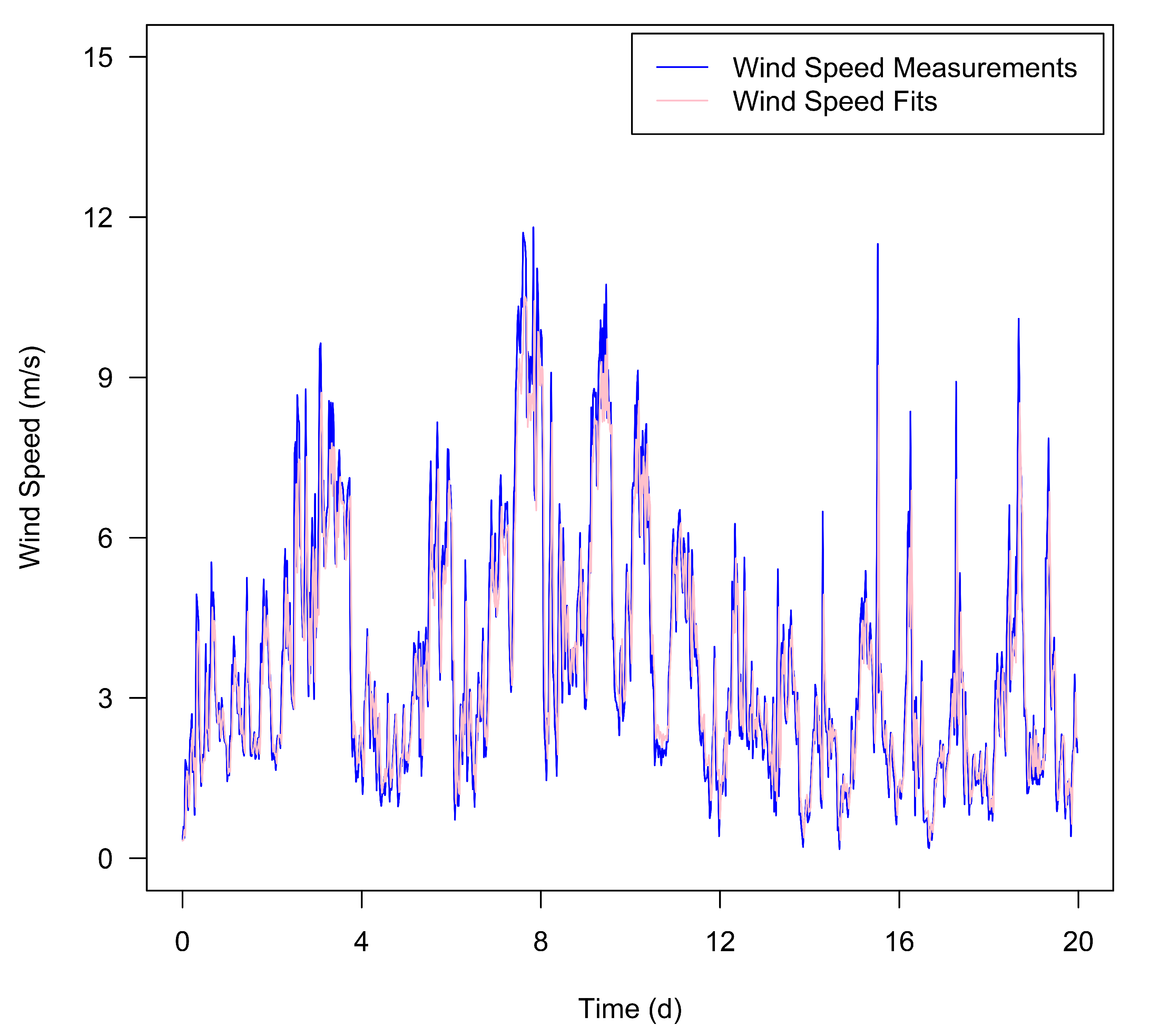
Energies 15 05472 g005
Figure 6. Comparison between the wind speed fits provided by the ARIMA ( 2 , 1 , 1 ) model and the historical wind speed measurements from the 20-day training dataset.
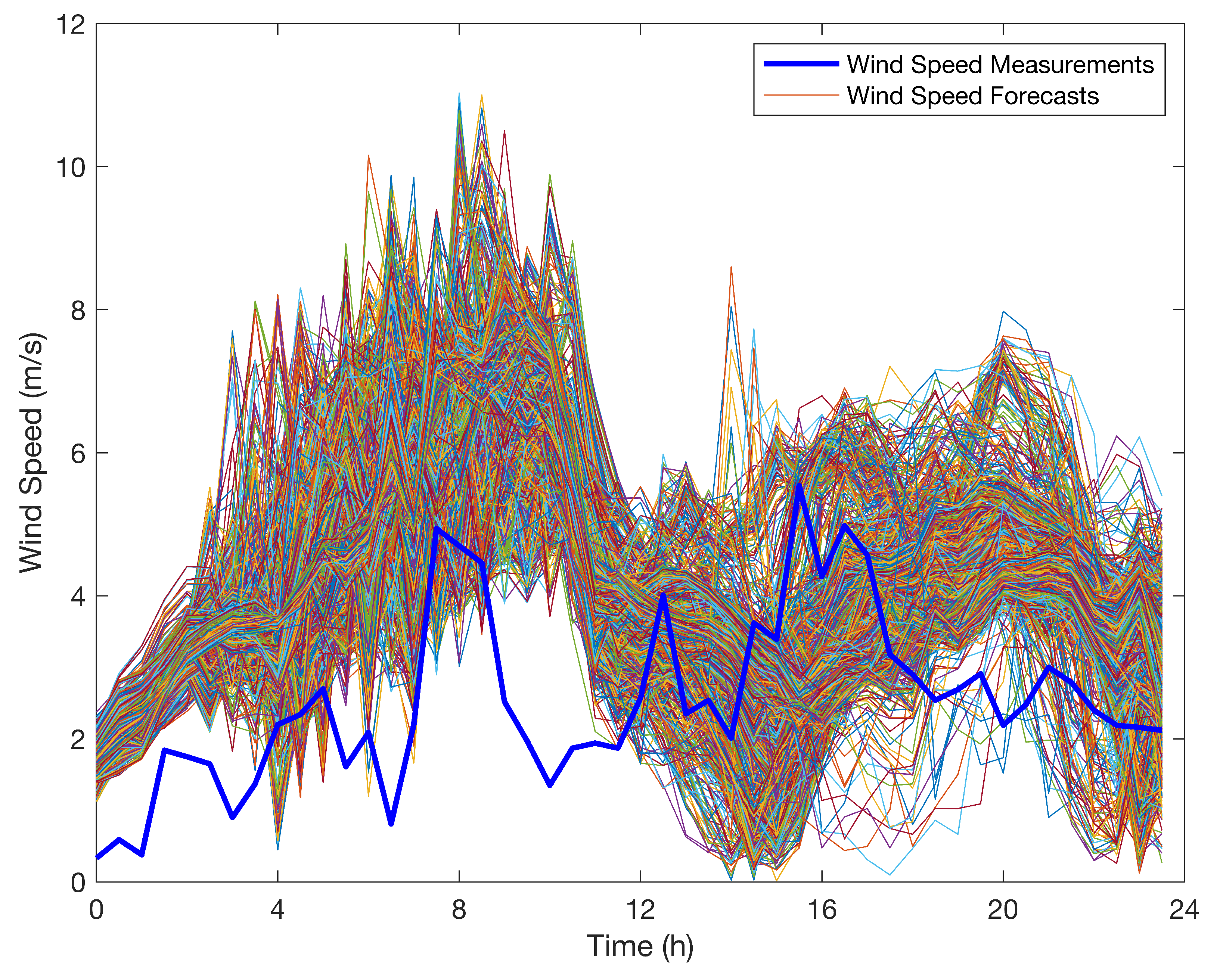
Energies 15 05472 g006
Figure 7. Comparison of the wind speed forecasts provided by the 1334 different WRF models and the historical wind speed measurements obtained on 11 August 2015 (the first day of the training dataset).
Energies 15 05472 g007
Figure 8. Comparison of the multi-hour ahead wind power forecasts provided by the proposed forecasting system and the historical wind power measurements from the 4-day test dataset.
Energies 15 05472 g008
Table 1. The various parameterisation schemes (used in this study) for each of the five physics options in the WRF model: the microphysics parameterisation (mp_physics), cumulus parameterisation (cu_physics), planetary boundary-layer parameterisation (bl_pbl_physics), surface-layer parameterisation (sf_sfclay_physics), and land-surface parameterisation (sf_surface_physics) [32].
Numbermp_physicscu_physicsbl_pbl_physicssf_sfclay_physicssf_surface_physics
1Purdue LinKain–FritschYonsei UniversityRevised MM5Rapid Update Cycle
2Ferrier EtaBetts–Miller–JanjicMellor–Yamada–JanjicEta SimilarityNoah-Multi-Physics
3WRF Single-Moment 6-ClassGrell–FreitasQuasi-Normal Scale EliminationQuasi-Normal Scale EliminationCommunity Land Model Version 4
4Thompson et al.Grell 3DMellor–Yamada Nakanishi and Niino Level 3Mellor–Yamada Nakanishi and Niino
5Milbrandt–Yau Double-Moment 7-ClassZhang–McFarlaneBouLacTotal Energy–Mass Flux
6Stony Brook University (Y. Lin)Kain–Fritsch–Cumulus PotentialUniversity of Washington
7WRF Double-Moment 6-ClassMulti-Scale Kain–FritschTotal Energy–Mass Flux
8NSSL Single-Moment 6-ClassNew TiedtkeShin–Hong
9NSSL-LFO Single-Moment 6-Class Grenier–Bretherton–McCaa
10Thompson Aerosol-Aware
Table 2. Four common types of criteria used in the technique for order of preference by similarity to ideal solution (TOPSIS) scheme and their characteristics.
TypeCharacteristic
Benefit criterionThe bigger, the better.
Cost criterionThe smaller, the better.
Intermediate criterionThe closer to a specific value, the better.
Interval criterionThe closer to a specific interval, the better.
Table 3. Segmental and overall rankings of the top six candidate WRF models as determined using the 20-day wind speed training dataset.
Model Index1st 4-Day2nd 4-Day3rd 4-Day4th 4-Day5th 4-Day20-Day
1212521
2123265
3471734
4556113
5344442
66354756
Table 4. Segmental and overall rankings of the 5-in-1 (ensemble) and top five WRF models as determined using the 20-day wind speed training dataset.
Model Index1st 4-Day2nd 4-Day3rd 4-Day4th 4-Day5th 4-Day20-Day
1223432
2334576
3581744
4667225
5455353
5-1112111
Table 5. Rankings of the 5-in-1 (ensemble) and top five WRF models in accordance with the similarity score as determined using the 4-day wind speed test dataset.
RankModel IndexSimilarity Score
130.9856
25-10.9641
340.9489
410.9447
550.7364
620.6197
Table 6. Evaluation results for the wind speed forecasting using the corrected and original 5-in-1 (ensemble) WRF models applied to the 4-day test dataset.
ModelMB (m·s 1 )MAE (m·s 1 )RMSE (m·s 1 )IAMAPESMAPE
Corrected 5-in-1 (ensemble) WRF model0.211.071.350.8953.71%36.73%
Original 5-in-1 (ensemble) WRF model0.701.291.610.8364.59%42.15%
Table 7. Four-day average mean bias for the wind speed forecasting using the persistence, autoregressive integrated moving average (ARIMA), and WRF-TOPSIS models applied to the 4-day test dataset.
4-Day Average MB (m·s 1 )Persistence ModelARIMA ModelWRF-TOPSIS Model
Forecast30 min−0.01−0.140.21
1 h−0.03−0.200.21
1.5 h−0.05−0.290.21
time2 h−0.05−0.310.21
3 h−0.11−0.280.21
4 h−0.18−0.450.21
horizon6 h−0.32−0.320.21
8 h−0.42−0.670.21
12 h−0.57−0.590.21
24 h−0.42−0.780.21
Table 8. Four-day average mean absolute error for the wind speed forecasting using the persistence, ARIMA, and WRF-TOPSIS models applied to the 4-day test dataset.
4-Day Average MAE (m·s 1 )Persistence ModelARIMA ModelWRF-TOPSIS Model
Forecast30 min0.610.611.07
1 h0.830.721.07
1.5 h0.990.831.07
time2 h1.100.951.07
3 h1.220.951.07
4 h1.411.061.07
horizon6 h1.621.321.07
8 h1.781.371.07
12 h2.221.491.07
24 h2.161.441.07
Table 9. Four-day average root mean squared error for the wind speed forecasting using the persistence, ARIMA, and WRF-TOPSIS models applied to the 4-day test dataset.
4-Day Average RMSE (m·s 1 )Persistence ModelARIMA ModelWRF-TOPSIS Model
Forecast30 min0.910.911.35
1 h1.241.051.35
1.5 h1.451.241.35
time2 h1.541.361.35
3 h1.681.371.35
4 h1.861.501.35
horizon6 h2.071.671.35
8 h2.321.771.35
12 h2.771.921.35
24 h2.671.911.35
Table 10. Four-day average index of agreement for the wind speed forecasting using the persistence, ARIMA, and WRF-TOPSIS models applied to the 4-day test dataset.
4-Day Average IAPersistence ModelARIMA ModelWRF-TOPSIS Model
Forecast30 min0.940.950.89
1 h0.890.930.89
1.5 h0.860.900.89
time2 h0.850.890.89
3 h0.830.890.89
4 h0.800.880.89
horizon6 h0.770.850.89
8 h0.720.850.89
12 h0.640.830.89
24 h0.670.840.89
Table 11. Four-day average mean absolute percentage error for the wind speed forecasting using the persistence, ARIMA, and WRF-TOPSIS models applied to the 4-day test dataset.
4-Day Average MAPEPersistence ModelARIMA ModelWRF-TOPSIS Model
Forecast30 min22.86%23.31%53.71%
1 h31.46%27.76%53.71%
1.5 h38.37%30.53%53.71%
time2 h42.70%36.57%53.71%
3 h53.43%36.85%53.71%
4 h61.19%42.36%53.71%
horizon6 h69.59%55.50%53.71%
8 h80.40%54.16%53.71%
12 h98.38%60.58%53.71%
24 h89.47%52.67%53.71%
Table 12. Four-day average symmetric mean absolute percentage error for the wind speed forecasting using the persistence, ARIMA, and WRF-TOPSIS models applied to the 4-day test dataset.
4-Day Average SMAPEPersistence ModelARIMA ModelWRF-TOPSIS Model
Forecast30 min21.68%21.47%36.73%
1 h28.47%24.92%36.73%
1.5 h33.58%27.49%36.73%
time2 h37.59%32.22%36.73%
3 h42.53%30.76%36.73%
4 h49.11%36.35%36.73%
horizon6 h55.76%42.97%36.73%
8 h59.11%45.63%36.73%
12 h71.62%47.73%36.73%
24 h67.38%46.28%36.73%
Table 13. Four-day average mean bias for the wind power forecasting using the direct persistence, indirect persistence-ANFIS, ARIMA-ANFIS, and WRF-TOPSIS-ANFIS models applied to the 4-day test dataset.
4-Day Average MB (kW)Direct Persistence ModelIndirect Persistence-ANFIS ModelARIMA-ANFIS ModelWRF-TOPSIS-ANFIS Model
Forecast30 min−1.4−0.5−24.0−16.6
1 h−2.8−2.0−33.3−16.6
1.5 h−3.7−3.0−45.7−16.6
time2 h−4.7−4.0−49.5−16.6
3 h−9.6−9.1−49.7−16.6
4 h−17.3−17.1−63.6−16.6
horizon6 h−31.2−31.5−64.7−16.6
8 h−38.7−39.7−89.6−16.6
12 h−48.5−49.7−87.1−16.6
24 h−38.7−40.0−104.6−16.6
Table 14. Four-day average mean absolute error for the wind power forecasting using the direct persistence, indirect persistence-ANFIS, ARIMA-ANFIS, and WRF-TOPSIS-ANFIS models applied to the 4-day test dataset.
4-Day Average MAE (kW)Direct Persistence ModelIndirect Persistence-ANFIS ModelARIMA-ANFIS ModelWRF-TOPSIS-ANFIS Model
Forecast30 min48.650.849.077.8
1 h69.168.457.277.8
1.5 h80.379.868.977.8
time2 h87.587.674.077.8
3 h95.595.178.377.8
4 h107.4105.777.177.8
horizon6 h116.4115.4100.577.8
8 h129.1126.798.677.8
12 h157.3155.2111.877.8
24 h161.4159.5110.277.8
Table 15. Four-day average root mean squared error for the wind power forecasting using the direct persistence, indirect persistence-ANFIS, ARIMA-ANFIS, and WRF-TOPSIS-ANFIS models applied to the 4-day test dataset.
4-Day Average RMSE (kW)Direct Persistence ModelIndirect Persistence-ANFIS ModelARIMA-ANFIS ModelWRF-TOPSIS-ANFIS Model
Forecast30 min104.7104.7104.4129.8
1 h139.8138.9115.0129.8
1.5 h158.2157.6137.0129.8
time2 h167.7166.7142.8129.8
3 h178.7177.5150.5129.8
4 h191.7189.5154.4129.8
horizon6 h197.9194.9169.6129.8
8 h214.6210.5179.0129.8
12 h242.2237.7193.4129.8
24 h259.1254.0195.6129.8
Table 16. Four-day average index of agreement for the wind power forecasting using the direct persistence, indirect persistence-ANFIS, ARIMA-ANFIS, and WRF-TOPSIS-ANFIS models applied to the 4-day test dataset.
4-Day Average IADirect Persistence ModelIndirect Persistence-ANFIS ModelARIMA-ANFIS ModelWRF-TOPSIS-ANFIS Model
Forecast30 min0.820.820.780.66
1 h0.660.650.730.66
1.5 h0.560.550.540.66
time2 h0.530.530.530.66
3 h0.540.540.520.66
4 h0.410.410.500.66
horizon6 h0.420.420.400.66
8 h0.330.340.400.66
12 h0.180.180.340.66
24 h0.210.210.380.66
Table 17. Four-day average accuracy rate for the wind power forecasting using the direct persistence, indirect persistence-ANFIS, ARIMA-ANFIS, and WRF-TOPSIS-ANFIS models applied to the 4-day test dataset.
4-Day Average Accuracy RateDirect Persistence ModelIndirect Persistence-ANFIS ModelARIMA-ANFIS ModelWRF-TOPSIS-ANFIS Model
Forecast30 min93.02%93.02%93.04%91.35%
1 h90.68%90.74%92.33%91.35%
1.5 h89.45%89.49%90.86%91.35%
time2 h88.82%88.89%90.48%91.35%
3 h88.09%88.17%89.96%91.35%
4 h87.22%87.37%89.71%91.35%
horizon6 h86.81%87.01%88.69%91.35%
8 h85.69%85.97%88.06%91.35%
12 h83.85%84.15%87.11%91.35%
24 h82.73%83.07%86.96%91.35%
Table 18. Four-day average qualification rate for the wind power forecasting using the direct persistence, indirect persistence-ANFIS, ARIMA-ANFIS, and WRF-TOPSIS-ANFIS models applied to the 4-day test dataset.
4-Day Average Qualification RateDirect Persistence ModelIndirect Persistence-ANFIS ModelARIMA-ANFIS ModelWRF-TOPSIS-ANFIS Model
Forecast30 min98.96%98.96%99.48%97.92%
1 h97.40%97.40%98.96%97.92%
1.5 h96.35%96.35%97.92%97.92%
time2 h96.35%96.35%96.88%97.92%
3 h93.75%93.23%96.35%97.92%
4 h92.19%93.75%96.35%97.92%
horizon6 h94.79%94.79%93.75%97.92%
8 h90.62%91.15%94.27%97.92%
12 h90.10%90.62%92.19%97.92%
24 h88.54%89.06%92.19%97.92%
Table 19. Model rankings for each forecast time horizon according to the similarity score.
Similarity ScoreRank 1Rank 2Rank 3Rank 4
Forecast30 minDirect persistence model (0.9727)Indirect persistence-ANFIS model (0.9617)ARIMA-ANFIS model (0.5034)WRF-TOPSIS-ANFIS model (0.2039)
1 hARIMA-ANFIS model (0.7086)Indirect persistence-ANFIS model (0.3620)Direct persistence model (0.3433)WRF-TOPSIS-ANFIS model (0.3414)
1.5 hARIMA-ANFIS model (0.7177)WRF-TOPSIS-ANFIS model (0.5111)Indirect persistence-ANFIS model (0.2546)Direct persistence model (0.2435)
time2 hWRF-TOPSIS-ANFIS model (0.8042)ARIMA-ANFIS model (0.6587)Indirect persistence-ANFIS model (0.2701)Direct persistence model (0.2649)
3 hWRF-TOPSIS-ANFIS model (0.9391)ARIMA-ANFIS model (0.6067)Indirect persistence-ANFIS model (0.2732)Direct persistence model (0.2656)
4 hWRF-TOPSIS-ANFIS model (0.9865)ARIMA-ANFIS model (0.6230)Indirect persistence-ANFIS model (0.2713)Direct persistence model (0.2602)
horizon6 hWRF-TOPSIS-ANFIS model (1.0000)ARIMA-ANFIS model (0.3744)Indirect persistence-ANFIS model (0.2071)Direct persistence model (0.2013)
8 hWRF-TOPSIS-ANFIS model (1.0000)ARIMA-ANFIS model (0.4394)Indirect persistence-ANFIS model (0.2206)Direct persistence model (0.2133)
12 hWRF-TOPSIS-ANFIS model (1.0000)ARIMA-ANFIS model (0.4237)Indirect persistence-ANFIS model (0.1911)Direct persistence model (0.1898)
24 hWRF-TOPSIS-ANFIS model (1.0000)ARIMA-ANFIS model (0.4805)Indirect persistence-ANFIS model (0.2191)Direct persistence model (0.2163)
Table 20. Evaluation results of the multi-hour ahead wind power forecasting system applied to the 4-day test dataset.
Metric30 min to 24 h (Every 30 min)
MB (kW)−16.6
MAE (kW)77.8
RMSE (kW)129.8
IA0.66
Accuracy rate91.35%
Qualification rate97.92%
Publisher’s Note: MDPI stays neutral with regard to jurisdictional claims in published maps and institutional affiliations.

