Energy Loss Reduction for Distribution Networks with Energy Storage Systems via Loss Sensitive Factor Method

Abstract

The loss of distribution networks caused by various electrical motors including transformers and generators can significantly affect the efficiency and economical operation of the power grid, especially for new power systems with high penetration of renewable energies. In this paper, the potential of using an energy storage system (ESS) for loss reduction is investigated, where a novel two-stage method for key-bus selection and ESS scheduling is proposed. At the first stage, the most sensitive key buses to the variation of load are selected by using the loss sensitive factors (LSF) method. At the second stage, ESS scheduling is conducted by solving an optimization problem with uncertainties caused by high penetration of renewable energies, where the uncertainties are characterized by confidence levels. The optimal scheduling of ESS including locations, capacities, and working modes are obtained at the second stage. The effectiveness of the proposed method is demonstrated via numerical simulations. The influences of capacities of ESS and confidence levels with respect to uncertainties are also analyzed. It is demonstrated that the loss-reduction performances can be improved if the ESSs are deployed on the buses selected by the LSF method and operated under the developed optimal scheduling method.

1. Introduction

The efficiency of energy conversion and transmission is of great significance for the operation of power systems, where energy saving and loss reduction constitutes an important part of energy utilization and economic development. They can mainly be divided into two main parts, the management loss and the technical loss, where the former is induced by the transgression in using electricity and statistical errors [1]; the latter is composed of the variable loss and constant loss of power systems [2]. Various motors including transformers and generators are indispensable components of the distribution networks with unavoidable losses such as the copper and iron loss. A large amount of eddy current loss is generated due to the air gap of a generator which yields higher-order harmonics with the rotating rotor in relative motion [3]. Core losses and winding losses are common for transformers. Proper loss management and loss reduction methods directly affect the efficiency and economy of distribution networks [4]. The loss reduction for distribution networks has drawn much attention, where both the optimization of active and reactive power [5,6] and the improvement of distribution network structures [7,8,9] have been studied. Li et al. [7] studied the economic dispatch problem in a smart grid, where a fully distributed algorithm was introduced to schedule generators. In [8], a combined optimization model for power loss reduction was proposed by improving distribution lines, transformers, and reactive power compensation. In [9], the annual energy loss was minimized through the integration of non-dispatchable renewable and network reconfiguration under varying load demand circumstances.

With the rapid development of new power systems with high penetration of renewable energies, the strong intermittency and randomness of renewable energies yields great challenges for the loss management and reduction of distribution networks [10,11]. For renewable energies dominated distribution networks, the equivalent load (EL) supported by the generators of the main grid would be frequently fluctuated due to the seasonal-fluctuated outputs of renewable energies. As a result, it is difficult for the generators to keep up with the changes in EL, which in turn leads to frequency fluctuations and voltage quality problems in distribution networks, increasing energy losses in the networks. The loss reduction and optimization for distribution systems with high penetration of renewable energies has drawn much attention. Adefarati et al. [12] pointed out that improper sizing, location and poor planning of renewable units can cause excessive power losses and feeders overload. In [13], a method based on generating a probabilistic generation-load was proposed by optimally allocating different types of renewable distributed generation to minimize energy losses. In [14], the influence of reactive power resources of distributed energy on loss reduction was studied. Alturki et al. [15] studied the line loss and power transmission in conjunction with the operating characteristics of the power grid, and proposed a control method power transmission to reduce the loss.

The energy storage systems (ESS) play an important role in smoothing the fluctuations of renewable energy sources [16], such as wind turbine (WT) and photovoltaic (PV). They can compensate well for load fluctuations caused by generators and transmission loss on the source side. In [17], it was found that energy loss can be effectively reduced by using ESS to balance the power exchange, where the efficiency of loss reduction was influenced by the locations and the size of ESS. Therefore, the location selection and optimal scheduling are two key points for loss reduction with ESS. Reference [18] demonstrated that there was always an optimal capacity allocation scheme when the generation cost curve was convex. Swarm intelligent optimization algorithms were employed for key location selection of ESS [17,19,20,21]. In [22], a cost-based approach was proposed to optimize the location and capacity of ESS. In [23], the difference between the minimal and maximal loss sensitive factors (LSF) value were adopted for location selection. Moreover, the efficient and reliable configuration of ESS are important forESS schedulings. In [17], a linear mixed-integer cost model was constructed to determine the location and capacity of ESS and capacitors, resulting in the improvement of the network reliability and and reduction of loss. In [24], the efficiency of the ESS optimal model was evaluated, and various scenarios for capacity increment of ESS was considered. In [25], a bi-level decision architecture was proposed for optimal allocation of ESS.

Note that for the new power system with high penetration of renewable energies, ESS are essential and dispensable to smooth the fluctuations of renewable energy sources. However, the loss reduction function by using ESS has not been fully studied. Due to the high cost of ESS facilities, it is essential to devise an efficient way of using ESS resources for the purpose of loss reduction, where the ESS facilities should be equipped at the most efficient locations and be operated under the most time-efficient working modes to avoid complete occupation of the ESS resources. Although several location selection and optimal scheduling methods have been developed, the integrated management issues for ESS including the location selection, optimal scheduling, and working modes have not been fully addressed. This motivates the study of this paper.

In this paper, to explore the loss-reduction potential of using ESS for new power systems with high penetration of renewable energies. A two-stage method is proposed for the integrated management of ESS including the location selection, optimal scheduling and working modes selection. The first stage is the key-bus selection problem, where the most efficient ESS locations are selected by using the peak LSF method. The LSF method has been known as one of the reliable methods for determining the optimal location of distributed generation in the distribution network [26]. The peak LSF method calculates the LSF value during the highest load time of day, indicating the most sensitive buses to loss of electrical facilities. The second stage is the optimal scheduling problem for ESS, where the uncertainties of renewable energies are considered and different working modes of the ESS are studied. Extensive numerical simulations are conducted to demonstrate the effectiveness of the proposed method.

The main contributions of this paper are summarized as follows:

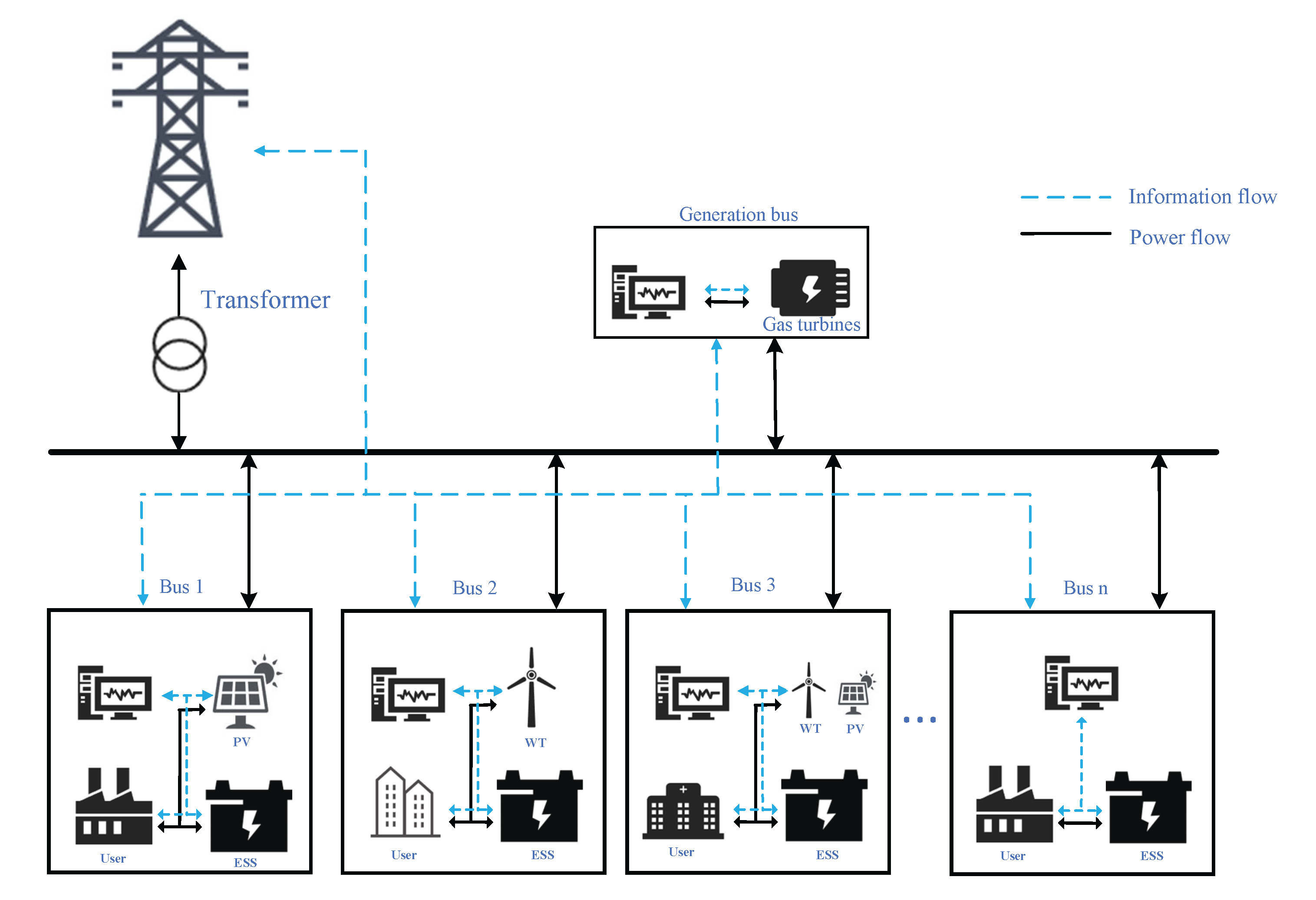
• A two-stage method is proposed to explore the loss-reduction potential of using ESS for new power systems with high penetration of renewable energies, where the integrated management of ESS including the location selection, optimal scheduling, and working modes selection is considered.
• For the ESS scheduling problem, the uncertainties of renewable energies are formulated as confidence levels with probability constraints and transformed into deterministic constraints through the chance constraint programming method.
• Various ESS usage scenarios are analyzed, including co-working of multiple ESS, working modes of ESS, and the influence of the ESS capacities. Extensive numerical simulations based on IEEE 33 standard distribution system are conducted to demonstrate the effectiveness of the proposed method.

2. Main Results

2.1. Problem Formulation

The distribution network considered in this paper is a radial distributed one as shown in Figure 1, where both conventional energy generators such as gas turbines and renewable energy sources including WT and PV are included at different buses. Due to the strong randomness and fluctuation of renewable energies, ESS are necessary and would be equipped at some buses of the distribution networks. This paper explores the loss-reduction potential of using ESS for the radial distributed systems. Considering the high cost of ESS facilities, the efficiency of using ESS facilities is particularly concerned, where the problem of maximizing the loss reduction with minimal ESS resources and working modes is studied by proposing a two-stage method as presented at Section 2.2. For the proposed two-stage method, to minimize the adopted ESS resources, the most efficient buses for the loss-reduction performance of ESS will be identified (stage one in Section 2.3). Moreover, the optimal scheduling problem with different working modes for the ESS deployed at the identified key buses will be studied (stage two in Section 2.4).

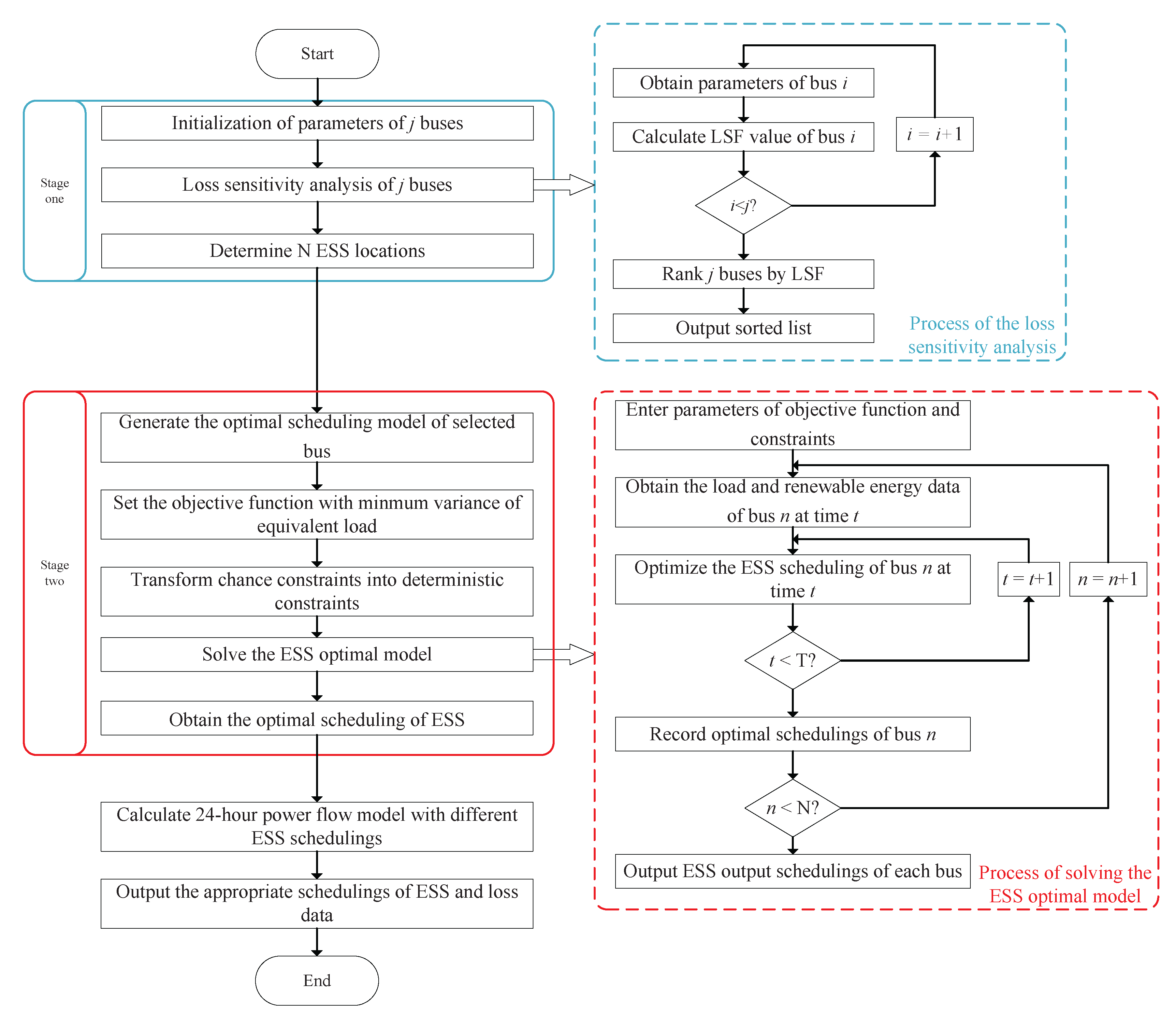
2.2. The Proposed Two-Stage Method

The flow chart of the proposed two-stage method is shown in Figure 2. In the first stage, the LSF values at peak hours are calculated and adopted for the key-bus location selection. In the second stage, an integrated model including the uncertainties caused by the fluctuation of renewable energies is formulated and solved by using the chance constraint method, where the minimal EL fluctuation is adopted as the optimization objective. In what follows, the two stages will be described in detail in Section 2.3 and Section 2.4, respectively.

2.3. Stage One: Key-Bus Location Selection

The loss-reduction efficiency for each bus is influenced by the R/X ratio, the active and reactive powers, and the topology of the distribution network. In this stage, an LSF-based key-bus selection method is established.

Consider a specific bus i, and assume that no load is included in the buses except the bus i. Thus, from the superposition principle, the entire loss can be calculated as follows [27]

$$\Delta P_{si}=\frac{P_i^2+Q_i^2}{U_i^2}\sum R_{si}$$

(1)

where $\Delta P_{si}$ is the loss from the root bus s to bus i; $P_i$ and $Q_i$ are the active power and reactive power of bus i, respectively; $U_i$ is the voltage amplitude of bus i; $\Sigma R_{si}$ is the equivalent resistance from the root bus s to the bus i.

Similarly, one obtains the active loss from bus i to bus s as follows

$$\Delta P_{is}={\left(U_s-U_i\right)}^2\sum G_{si}=\frac{{\left(P_i\sum R_{si}+Q_i\sum X_{si}\right)}^2}{U_i^2\sum R_{si}}$$

(2)

From Equations (1) and (2), by using $\Delta P_{si}=\Delta P_{is}$, one has

$$\frac{P_i^2+Q_i^2}{U_i^2}\sum R_{si}=\frac{{\left(P_i\sum R_{si}+Q_i\sum X_{si}\right)}^2}{U_i^2\sum R_{si}}$$

(3)

Then, $\Delta P_{si}$ can be represented as

$$\Delta P_{si}=\frac{1}{2}\times \left(\frac{P_i^2+Q_i^2}{U_i^2}\sum R_{si}+\frac{{\left(P_i\sum R_{si}+Q_i\sum X_{si}\right)}^2}{U_i^2\sum R_{si}}\right)$$

(4)

To minimize the loss, take the partial derivative of $\Delta P_{si}$ with respect to $\sum R_{si}$, and set the partial derivative as zero as follows

$$\frac{\partial \Delta P_{si}}{\partial \sum R_{si}}=0$$

(5)

Equation (5) can be represented as

$$\left(P_i^2+Q_i^2\right)\sum R_{si}^2={\left(P_i\sum R_{si}+Q_i\sum X_{si}\right)}^2-2P_i\sum R_{si}\times \left(P_i\sum R_{si}+Q_i\sum X_{si}\right)$$

(6)

The LSF value, that is $F_i$, is defined as the difference between the left and right sides of Equation (6). Furthermore, $F_i$ can be rewritten as

$$F_i=\sqrt{|\left(P_i^2+Q_i^2\right)·\sum R_{si}^2+2P{}_i\sum R_{si}·\left(P_i\sum R_{si}+Q_i\sum X_{si}\right)-{\left(P_i\sum R_{si}+Q_i\sum X_{si}\right)}^2|}$$

(7)

The LSF values ($F_i,i=1,\dots ,n$) from Equation (7) imply the sensitivity of the loss of the corresponding bus with respect to the variation of electric facilities. Therefore, they can be used to determine the key buses for equipping ESS.

2.4. Stage Two: Optimal Scheduling of ESS

2.4.1. Objective Function

The ESS scheduling problem can be formulated as a nonlinear optimization problem. The objective function of the optimal model is formulated to minimize the variance of equivalent load J, which is shown as follows

$$minJ=\sum _{t=1}^T{\left(P_t^{\mathrm{load}}+P_t^{\mathrm{new}}-P_t^{\mathrm{ess}}-P_t^{\mathrm{ave}}\right)}^2$$

(8)

$$P_t^{\mathrm{ave}}=\sum _{t=1}^T(P_t^{\mathrm{load}}+P_t^{\mathrm{ess}}-P_t^{\mathrm{new}})/T$$

(9)

where J denotes the variance of equivalent load; $P_t^{\mathrm{load}}$ and $P_t^{\mathrm{ess}}$ are the active power and charging-discharging power during hour t, respectively; $P_t^{\mathrm{ave}}$ is the averaged equivalent load; $P_t^{\mathrm{new}}$ is the renewable power output, which depends on the renewable energy devices configured at bus i.

2.4.2. Equivalent Load Model

In order to facilitate the integration of multiple random variables, the power of an equivalent load is composed of the following folds: the gross active power of the distribution network, the joint renewable power output of WT and PV, and the charging-discharging of ESS outputs. The total equivalent load can be represented as

$$P_t^{\mathrm{el}}=P_t^{\mathrm{load}}+P_t^{\mathrm{ess}}-P_t^{\mathrm{new}}$$

(10)

where $P_t^{\mathrm{el}}$ denotes the power of the equivalent load.

2.4.3. Capacity Constraint

The storage capacity constraint of the ESS is considered as follows

$$S_t^{\mathrm{ess}}=\left\{\begin{array}{c}{S}_{t-1}^{\mathrm{ess}}-\left|P_t^{\mathrm{ess}}\right|,\mathrm{in}\mathrm{discharge}\\ S_{t-1}^{\mathrm{ess}}+\left|P_t^{\mathrm{ess}}\right|,\mathrm{in}\mathrm{charge}\end{array}\right.$$

(11)

$$S_i^{min}⩽S_t^{\mathrm{ess}}⩽S_i^{max}$$

(12)

$$S_0^{\mathrm{ess}}=S_{24}^{\mathrm{ess}}$$

(13)

where $S_t^{\mathrm{ess}}$ and $S_{t-1}^{\mathrm{ess}}$ are the energy storage in hour t and $t-1$, respectively; $S^{min}$ and $S^{max}$ are the minimum and maximum energy storage of ESS, respectively. The minimum capacity $S^{min}$ of ESS is assumed to be $10\%$ of its own total capacity, i.e., the ESS stops working if the remaining capacity of ESS is lower than $S^{min}$.

2.4.4. Charging-Discharging Cycle Constraint

During the charging-discharging period, the ESS satisfies the following constraints:

$$P_t^{\mathrm{ess}}={\eta }^{ch}·P_t^{\mathrm{ess},\mathrm{ch}}-P_t^{\mathrm{ess},\mathrm{dis}}/{\eta }^{\mathrm{dis}}$$

(14)

$$0⩽P_t^{\mathrm{ess},\mathrm{ch}}⩽D_t^1·P_i^{\mathrm{ess},max}$$

(15)

$$0⩽P_t^{\mathrm{ess},\mathrm{dis}}⩽D_t^2·P_i^{\mathrm{ess},max}$$

(16)

$$D_t^1+D_t^2⩽1$$

(17)

where $P_t^{\mathrm{ess},\mathrm{ch}}$ and $P_t^{\mathrm{ess},\mathrm{dis}}$ are the charging power and dischagring power in hour t, respectively; $P^{\mathrm{ess},max}$ denotes the maximum charging-discharging power; $D_t^1$ and $D_t^2$ denotes the binary variable constraining the energy storage to be either charging or discharging.

2.4.5. PV Model and WT Model

The scheduling of ESS with uncertainties is of great interest and importance. In this paper, the model based on prediction and bias is employed.

The PV output can be expressed as the sum of the forecasted value and the forecasted error

$$P_t^{\mathrm{pv}}=0,\mathrm{nighttime}$$

(18)

$$P_t^{\mathrm{pv}}=P_t^{\mathrm{pv},\mathrm{f}}+{\epsilon }_t^{\mathrm{pv}},\mathrm{daytime}$$

(19)

where $P_t^{\mathrm{pv}}$ denotes the PV output in hour t; ${\epsilon }_t^{\mathrm{wt}}$ represents the prediction error in hour t, which is modeled as a normal distribution with zero mean, and standard deviation as follows

$${\sigma }_t^{\mathrm{pv}}=0.2P_t^{\mathrm{pv},\mathrm{f}}+0.02P_{cap}^{\mathrm{pv}}$$

(20)

where $P_{cap}^{\mathrm{pv}}$ denotes the installed PV capacity.

Similarly, the WT output can be expressed in the same way as follows

$$P_t^{\mathrm{wt}}=P_t^{\mathrm{wt},\mathrm{f}}+{\epsilon }_t^{\mathrm{wt}},1⩽t⩽24$$

(21)

where ${\epsilon }_t^{\mathrm{wt}}$ is independently and identically distributed with ${\epsilon }_t^{\mathrm{pv}}$.

2.4.6. Chance Constraint

In order to characterize the random factors of the renewable energies and load forecast errors, the power inequality of the system is expressed using the chance constraint, which comprises the following folds: the charging-discharging of ESS, the gross power load of the distribution network, the random renewable energy power outputs. The chance constraint can be presented as follows

$$Pr\left\{{\mathrm{P}}_{\mathrm{t}}^{\mathrm{g}}+{\mathrm{P}}_{\mathrm{t}}^{\mathrm{ess}}+{\mathrm{P}}_{\mathrm{t}}^{\mathrm{new}}⩾{\mathrm{P}}_{\mathrm{t}}^{\mathrm{load}}\right\}⩾\alpha$$

(22)

where $P_t^{\mathrm{g}}$ is the injected power of the generator units from the root bus, and is also the lowest power to guarantee the system stability; $\alpha$ is the confidence level.

The confidence level reflects the trade-off between efficiency of the distribution network and the risk of operation. When the confidence level is 1, it means that the network does not allow any potential risk of violating the constraint, which improves the stability of the network operation, but inevitably causes the waste of resources.

By using the method in [28], Equation (22) can be rewritten as follows

$$Pr\left\{-\left(P_t^{\mathrm{g}}+P_t^{\mathrm{ess}}-P_t^{\mathrm{load}}\right)⩽P_t^{\mathrm{new}}\right\}⩾K_{\alpha }$$

(23)

$$K={\Phi }^{-1}(1-\alpha )$$

(24)

where $P_t^{\mathrm{g}}$ and $P_t^{\mathrm{ess}}$ are random variables; $P_t^{\mathrm{new}}$ follows a normal distribution with the mean as ${\displaystyle \sum _{t=1}^T}{P}_t^{\mathrm{new}}$ and the standard deviation as ${\sigma }_t^{\mathrm{new}}$ and the specific value depend on the renewable energy configuration of bus i. $\Phi (·)$ is the distribution function of a random variable. ${\Phi }^{-1}(·)$ is the inverse function and may be multi-valued. Then, $K_{\alpha }$ can be represented as

$$K_{\alpha }=sup\left\{K\mid K={\Phi }^{-1}(1-\alpha )\right\}$$

(25)

3. Numerical Simulation

The IEEE 33 standard radial distribution network [29] added with WT units and PV units is adopted to verify the effectiveness of the proposed method. The structure of the distribution network mentioned above is shown in Figure 3. The load data is taken from [30], which is tailored and scaled to match the power flow features of the IEEE 33 standard radial distribution network. The root bus (bus 1) contains gas turbine generator units. Bus 30 and bus 25 contain renewable energy facilities. The parameters of the ESS and the generator type of each bus are given in

Table 1. The parameters of the ESS.

Parameter	Description	Value
$S_i^{max}$	Maximum energy storage at bus i	600 kW·h
$S_i^{min}$	Minimum energy storage at bus i	60 kW·h
$S_1^{\mathrm{ess}}$	Initial energy storage	300 kW·h
$P_t^{\mathrm{ch},max}$	Maximum charging power in hour t	100 kW
$P_t^{\mathrm{dis},min}$	Minimum discharging power in hour t	100 kW
${\eta }^{\mathrm{ch}}$	Charging efficiency	0.9
${\eta }^{\mathrm{dis}}$	Discharging efficiency	0.9
$\alpha$	Confidence level	0.95

and

Table 2. The LSF value, peak load, and generator type of each bus.

Bus	LSF Value	Peak Load/kW
30	4.38	209.4
32	3.27	233.8
25	2.56	424.3
14	2.32	122.8
18	2.23	90.5
31	2.02	149.3
7	1.15	210.8
8	1.33	231.1
24	1.93	420.5

, respectively. For each individual bus with renewable energy resources, the outputs of renewable energies accounts for 30% of the load on the bus. The Newton–Raphson power flow calculation method is adopted to iteratively calculate the output of the power and loss of the employed distribution network.

To demonstrate the effectiveness of the proposed two-stage method, the numerical simulation is conducted as follows. For the first stage, the LSF values are calculated according to Equation (7), where the buses with first six highest LSF values are shown in Table 2 (that is buses 32, 30, 25, 14, 18, and 31). The ESS facilities will be deployed according to the LSF values. Based on the results of stage one, for the second stage, the optimal scheduling of the ESS is conducted by solving a nonlinear optimization problem with uncertainties and three working modes.

The simulation results are presented as follows. Section 3.1 presents the simulation results of the key-bus selection and the ESS quantity selection. To show the effectiveness of the LSF method, a peak-load method is taken as comparison, where the ESSs are deployed as the first three highest load buses (buses 7, 8, and 24). Section 3.2 presents the loss-reduction performance analysis under three typical working modes listed in

Table 3. The typical working modes of ESS.

Working Mode	Description	Working Time
Mode I	9:00–21:00	Peak period
Mode II	7:00–19:00	Daytime period
Mode III	0:00–24:00	Whole day period

. In Section 3.3, the optimal scheduling analysis results are presented, where the optimal results, the influence of the capacities, and the influence of the confidence levels are analyzed.

Table 2 shows the LSF values and peak loads for typical buses calculated from Equation (7), where the detailed LSF values are given in Figure 4. According to Figure 4 and Table 2, the bus with the highest LSF value is bus 30 (the LSF value is 4.3817). The LSF value of bus 1 is 0 since it is a slack bus without power injection.

3.1. LSF-Based Key-Bus Location and Quantity Selection

The buses with the first six highest LSF values are shown in Table 2. To analyze the influence of the ESS quantity on the loss-reduction performance, six cases with different numbers of ESS equipped at the corresponding buses according to the LSF values in Table 2 in descending order are performed. The simulation results are shown in Figure 5, where one sees that for all working modes, the loss can be effectively reduced by increasing the quantity of ESS. However, the loss-reduction performance is not linearly improved with the quantity of the ESS, namely, for the cases with $n>3$, the loss does not reduce much compared to the cases with $n=3$. This means that the most suitable quantity of ESS is 3 which provides a balance between the cost and the performance.

Normally, a higher current could be generated if a higher load at a specific bus is connected, which tends to increase the overall loss of the distribution network system. Therefore, an intuitive bus selection method is to select the buses with higher loads. To quantitatively show the effectiveness of the proposed LSF method, a load group containing the buses with the first three highest loads is introduced for comparison (buses 7, 8, 24). Table 2 shows the parameters used in the buses selected by the LSF method and the high-load method, where for fair comparisons, the high-load group has the same capacity and types of renewable energy facilities as the LSF group.

Table 4. The loss information with different modes.

Bus	Working Mode	Average Loss/kW
		With ESS		Without ESS		Loss Reduction
		0:00–24:00	9:00–21:00	0:00–24:00	9:00–21:00	0:00–24:00	9:00–21:00
31, 30, 25 selected by the LSF method	Mode I	158.2849	188.5426	165.8027	198.1234	7.5178	9.5808
	Mode II	158.1085	187.0766			7.6942	11.0468
	Mode III	157.3428	182.2447			8.4599	15.8787
24, 7, 8 selected by the high-load method	Mode I	159.6283	190.326			6.1744	7.7974
	Mode II	159.4833	189.1896			6.3194	8.9338
	Mode III	158.9139	185.1232			6.8888	13.0002

shows the comparison of the average loss between the LSF method and the high-load method, where it can be seen that for each working mode or time period, more losses are reduced by the LSF method than the high-load method. For example, for Mode III, the average loss is reduced by $5.2\%$ (from 165.8027 kW to 157.3428 kW) in 0:00–24:00 via the LSF method; while the number for the high-load method is $4.1\%$ (from 165.8027 kW to 158.9139 kW). This demonstrates the effectiveness of the proposed LSF method in selecting key buses for loss reduction.

Another interesting finding is that Mode III and Mode II are better than Mode II and Mode I, respectively. This is understandable as longer working times are demanded. However, the improvements are not remarkable, implying that for the loss reduction purpose, the ESS takes only limited working times.

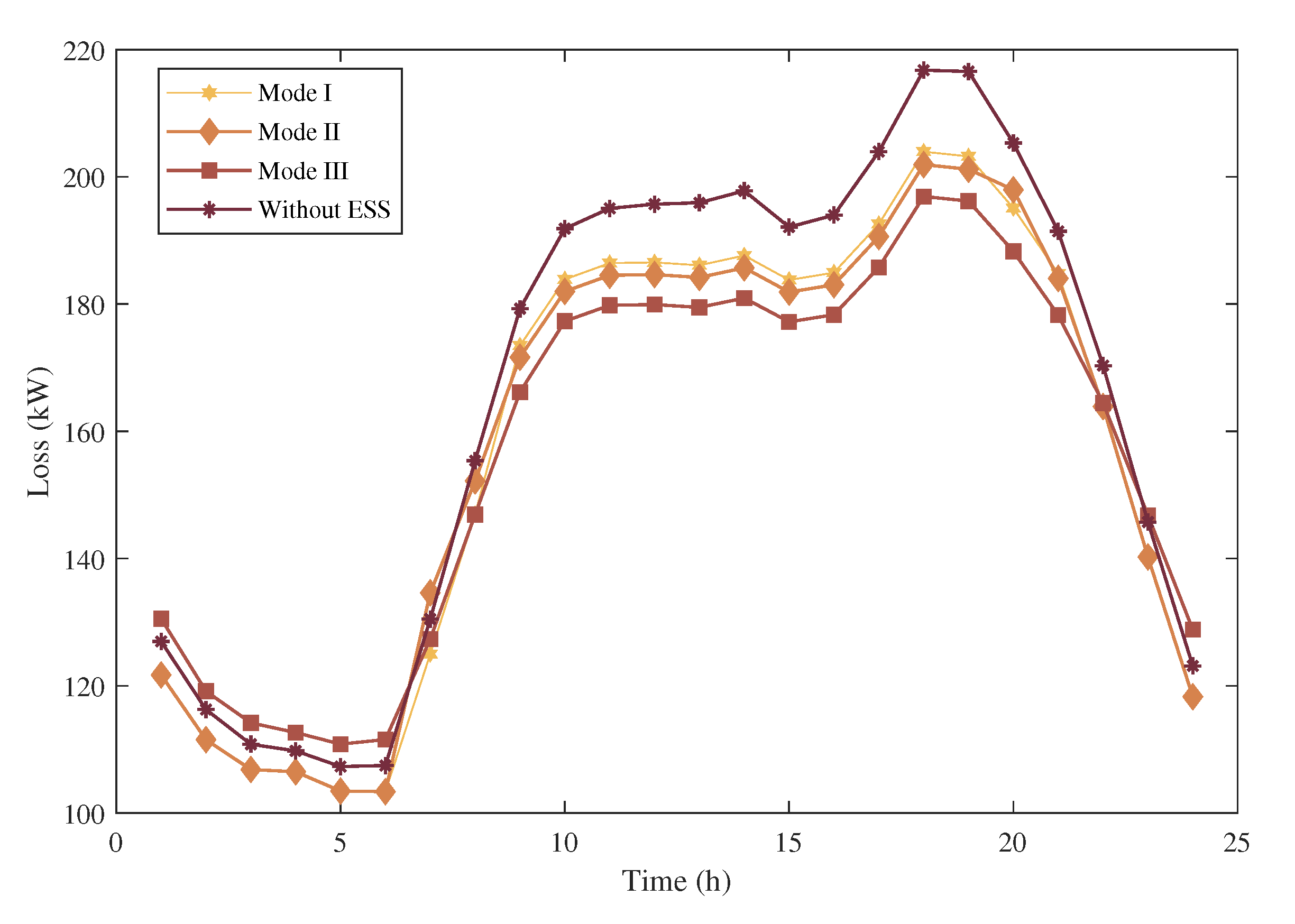
3.2. Loss-Reduction Performance Analysis

Figure 6 shows the variation of the loss in different modes where the three key buses (32, 30, 25) are selected based on the LSF method. It illustrates that ESS enables loss reduction for most of the day, which in turn saves energy. For most of the time, the loss in Mode III is the lowest among the three modes, and losses in Mode I and Mode II are lower than that of Mode III at 0:00–6:00. The losses in Mode I and Mode II are very close but higher than the one of Mode III. Similar to the findings of Table 4, Mode III performs the best due to the fact that most working time is required. The performances of Mode I and Mode II are very close.

Since Mode III performs the best among these working modes, Mode III is adopted to show the influence of the ESS’s capacities.

Table 5. The loss-reduction performance with different capacities and cases.

ESS Capacity/kW·h	Single ESS Case			Multiple ESSs Case
	30	32	25	32, 30, 25
400	162.263	165.2394	161.5967	158.0181
450	162.1864	165.2394	161.5643	157.8342
500	162.1119	165.2394	161.5329	157.6602
550	162.041	165.2394	161.5023	157.4986
600	161.9869	165.2394	161.4727	157.3428

reflects the loss-reduction performance of ESS with different capacities in Mode III. If multiple ESS are employed (selected by the LSF method), with the increase in capacities, more losses are reduced, although the reductions are not obvious. For the single ESS case (that is the ESS only deployed at the corresponding bus), it is observed that the variation of the capacity and location of ESS has little effect on the loss reduction performance. However, from Table 4, one sees that significant reduction can be achieved if multiple ESS are deployed. Compared with the single bus case, the power flow of the distribution network with multiple ESS is changed, resulting in significant reductions in the loss.

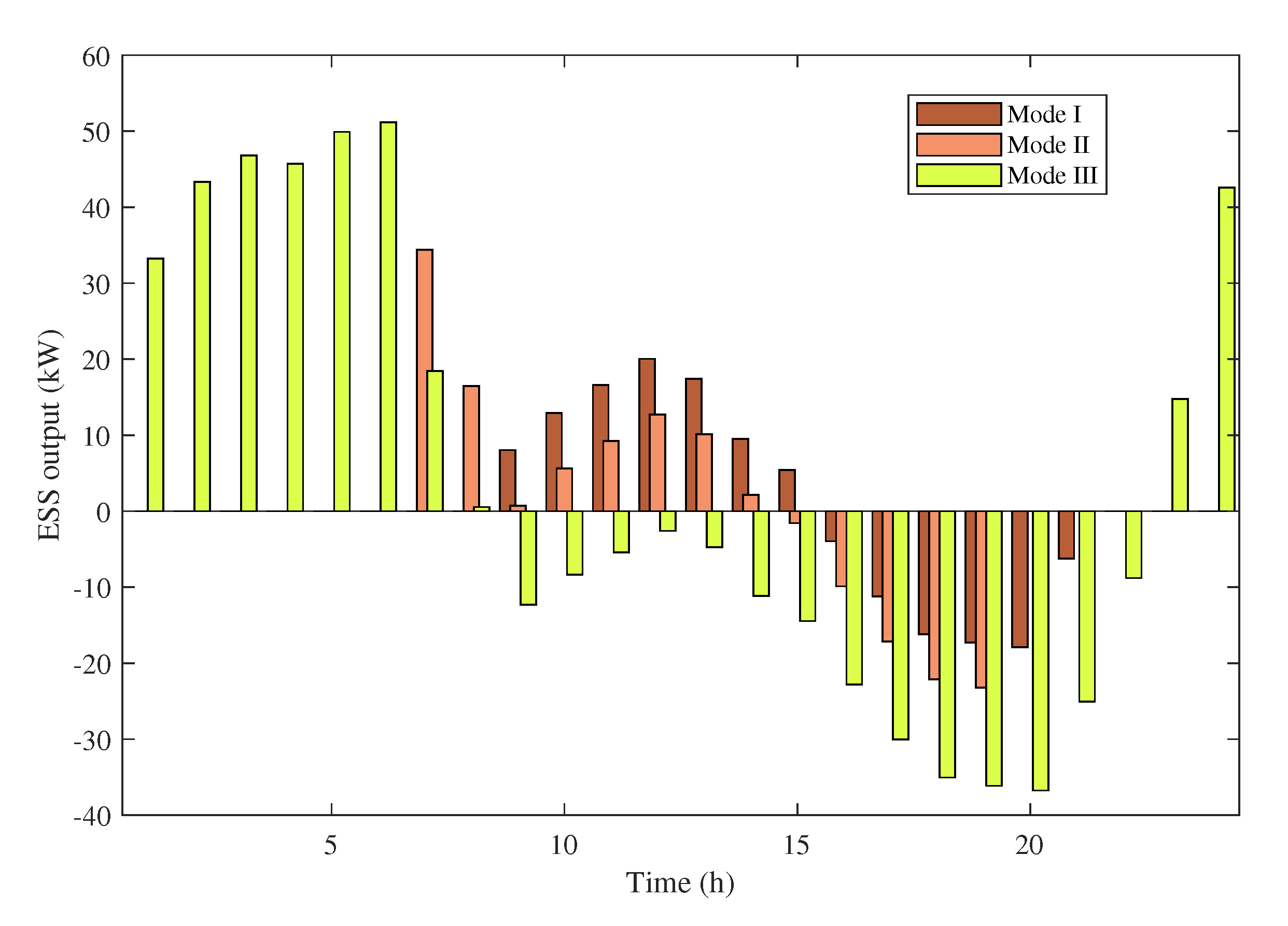
3.3. Optimal Scheduling Analysis

The EL curves and ESS charging-discharging schedulings with different modes are analyzed in this subsection, which explains the reasons why loss-reduction performance can be improved by optimizing the scheduling of ESS. In addition, the relationship between confidence levels and system stability is analyzed.

3.3.1. Optimal Results Analysis

Figure 7 shows the EL curves and the load curves for three working modes. As shown in Figure 7, the EL curves are relatively steady, demonstrating that ESS has the function of smoothing the curves. The EL curve of bus 25 is more drastic than the other two buses, which means that the EL curve may depend on the capacity of ESS.

Figure 8 shows the ESS outputs of bus 30 with different working modes. According to Figure 8, it is found that the ESS usually discharges during the peak load hours (9:00–21:00) and charges during the valley load hours (0:00–8:00) to keep the EL curves stable, which in turn decreases the loss of the distribution network. The charging behavior of ESS increases the load, which explains why the losses rise during the valley load hours.

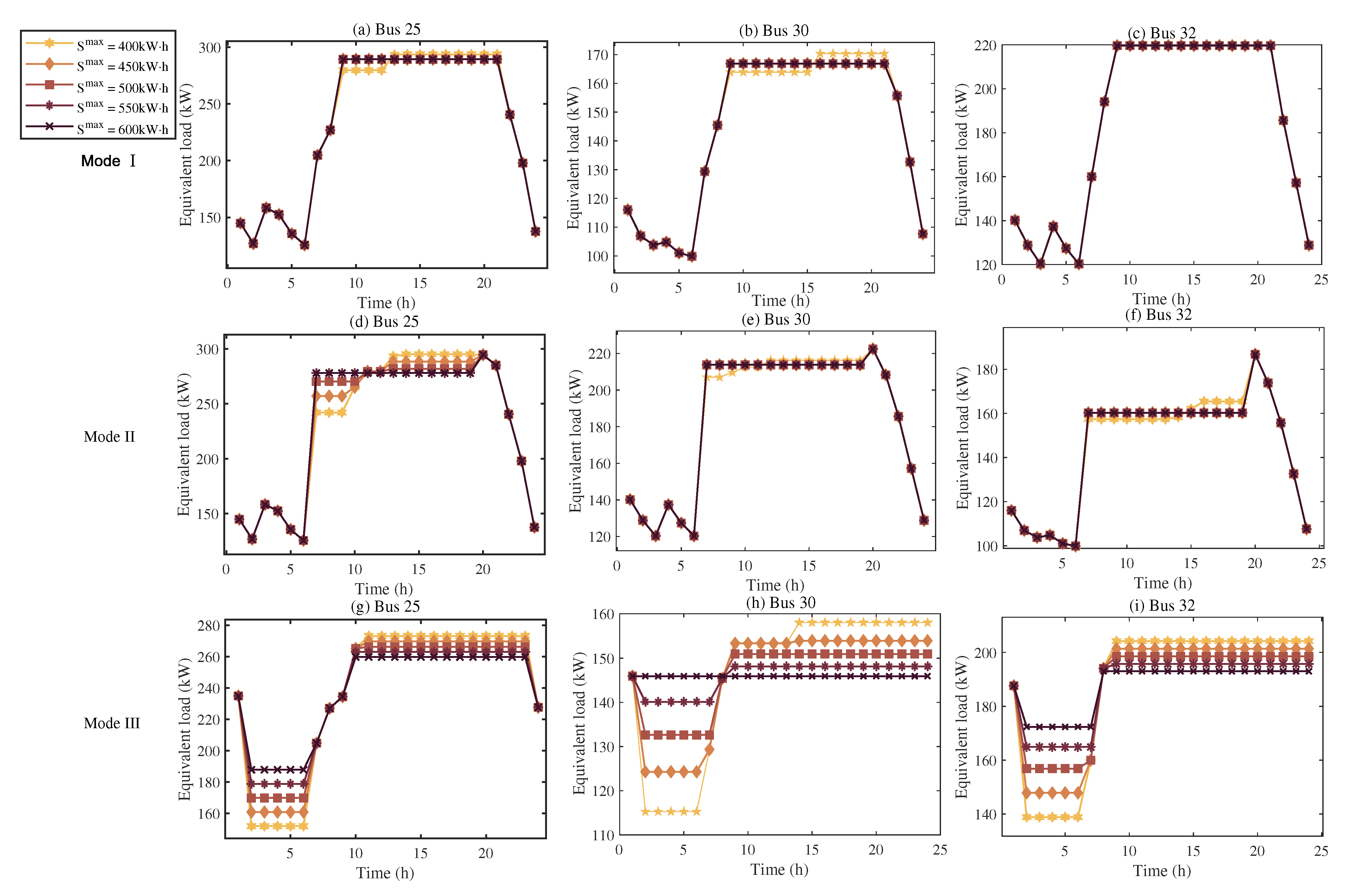
3.3.2. EL Curve Analysis with Different Capacities

Figure 9 shows the EL curves of buses with different working modes and capacities. As shown in Figure 9g–i, large ESS capacities tend to smooth the EL curves better. Combining with Table 5, the capacity of a single ESS optimizes the charging-discharging scheduling, which reduces the loss during the peak hours but raises the loss during the valley hours. Thus, for the single ESS case, increasing the capacity has little impact on loss reduction. However, for the multiple ESS case, it is shown that larger capacity can contribute to reducing more losses of the total distribution network, even though the reduction is not significant. For Figure 9b,e,h, for bus 30 with lower load, a stable EL curve can be obtained with small but suitable capacity of ESS.

Meanwhile, in contrast to Figure 9a,d,g, for bus 25, the EL curves fluctuate drastically during ESS non-working hours, while when ESS intervenes, the EL curve fluctuations are suppressed and maintained stable. Therefore, accordingly, in terms of the loss-reduction performance, the performance of Mode I and Mode II are worse than that of Mode III. It is well known that the cost of building and operating a large capacity ESS is normally demanded. Therefore, it is necessary to grasp the balance between the capacity and loss-reduction performance according to the actual situation. A proper capacity for ESS is essential for practical applications, and for this simulation, an ESS capacity of 500–600 kW·h is more appropriate.

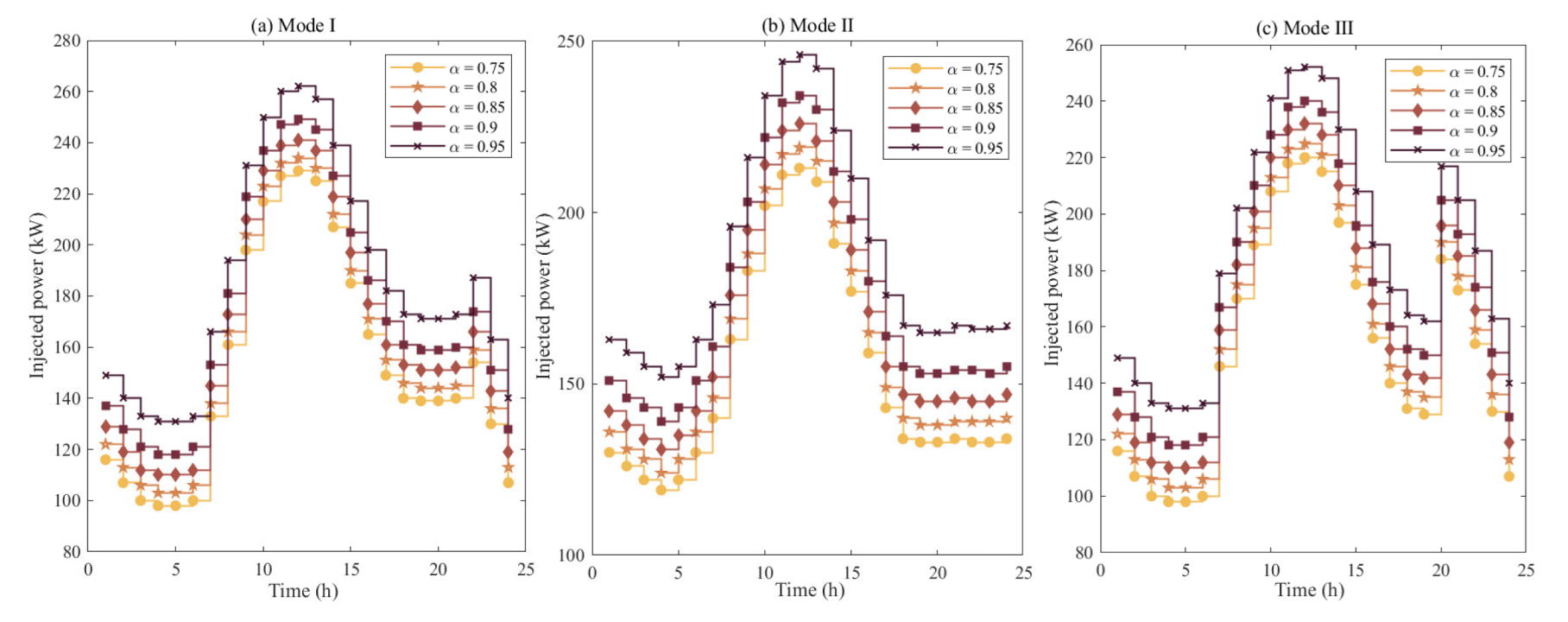
3.3.3. Confidence Levels Analysis

Due to the deployment of renewable energies including wind and solar powers, much of the uncertainties are depicted in the simulation. Figure 10 shows the injected power of bus 30 with different confidence levels. Note that the injected power increases with the increase of the loads and confidence levels. A higher confidence level indicates that the bus system is less tolerant to the risk, and a higher ability to control risk. To prevent the accidents such as exceedance of voltage limit and frequency fluctuations, additional energy needs to be injected to ensure the system operation safety. Thus, for Mode III, at 20:00–24:00, the load of the bus is suddenly increased because of the charging behavior of ESS, which in turn improves the injected power. An appropriate confidence level based on practical experience can be chosen to guarantee both system stability and loss-reduction performance.

4. Conclusions

This paper studied the loss-reduction problem by using ESS for distribution networks with high penetration of renewable energies, where multiple losses would be induced by various motors including transformers and generators. A two-stage method was proposed to address the integrated management issues for ESS including the key-bus selection, optimal scheduling, and working modes selection. For the first stage, an LSF-based key-bus selection was proposed; while for the second stage, the optimal scheduling of the ESS with uncertainties and various working modes was resolved. Numerical simulation based on the IEEE 33 radial distribution network was conducted to show the effectiveness of the proposed method. The main findings were summarized as follows:

1.

For the LSF-based key-bus selection method, it was found that although more losses can be reduced by increasing the quantity of ESS, there was a critical value for the number of ESS to balance the cost and the loss-reduction performance where negligible improvements would be obtained if the number of ESS exceeding the critical value (in the numerical simulation, the critical value is 3). Moreover, the proposed LSF method performed uniformly better than the high-load method in key-bus selection.

2.

Three typical working modes for the operation of ESS were studied, where it was found that the whole-day period working mode (Mode III) performed uniformly better than the other two working modes due to the fact that longer working time was adopted. However, the improvements were not significant as the most effective time for ESS to reduce loss was the peak period (from 9:00–21:00) which were also fully or partially covered by the other working modes.

3.

The influence of the capacities of the ESS on the loss-reduction performance was analyzed, where marginal improvements were obtained by increasing the ESS capacities. This means that the capacity was not the main factor affecting the loss-reduction performance. Moreover, the confidence level of the uncertainties induced by the renewable energies provided a balance between the risk tolerance and the system stability.

Although the effectiveness of the proposed two-stage method was demonstrated, the loss-reduction performance of ESS in the numerical simulation was marginally improved, which was not cost-effective compared with the high cost of ESS facilities. The problem of using surplus ESS capacities of existing ESS facilities to reduce energy loss will be studied in the future. Moreover, the line loading constraints were not included in the theoretical part of the proposed method, which will be considered in future work.

References

1. Usman, M.; Coppo, M.; Bignucolo, F.; Turri, R. Losses management strategies in active distribution networks: A review. Electr. Power Syst. Res. 2018, 163, 116–132. [Google Scholar] [CrossRef]
2. Passey, R.; Spooner, T.; MacGill, I.; Watt, M.; Syngellakis, K. The potential impacts of grid-connected distributed generation and how to address them: A review of technical and non-technical factors. Energy Policy 2011 39, 6280–6290. [CrossRef]
3. Chen, P.; Tang, R.; Tong, W.; Jia, J.; Duan, Q. Permanent magnet eddy current loss and its influence of high power density permanent magnet synchronous motor. Trans. China Electrotech. Soc. 2015, 30, 1–9. [Google Scholar]
4. Monteiro, R.V.A.; Bonaldo, J.P.; da Silva, R.F.; Bretas, A.S. Electric distribution network reconfiguration optimized for PV distributed generation and energy storage. Electr. Power Syst. Res. 2020, 184, 106319. [Google Scholar] [CrossRef]
5. Rajičić, D.; Todorovski, M. Participation of every generator to loads, currents, and power losses. IEEE Trans. Power Syst. 2020, 36, 1638–1640. [Google Scholar] [CrossRef]
6. Shaheen, A.M.; Elsayed, A.M.; El-Sehiemy, R.A.; Abdelaziz, A.Y. Equilibrium optimization algorithm for network reconfiguration and distributed generation allocation in power systems. Appl. Soft Comput. 2020, 98, 106867. [Google Scholar] [CrossRef]
7. Li, H.; Wang, Z.; Chen, G.; Dong, Z.Y. Distributed robust algorithm for economic dispatch in smart grids over general unbalanced directed networks. IEEE Trans. Ind. Inform. 2019, 16, 4322–4332. [Google Scholar] [CrossRef]
8. Xie, J.; Chen, C.; Long, H. A loss reduction optimization method for distribution network based on combined power loss reduction strategy. Complexity 2021, 2021, 9475754. [Google Scholar] [CrossRef]
9. Hesaroor, K.; Das, D. Annual energy loss reduction of distribution network through reconfiguration and renewable energy sources. Int. Trans. Electr. Energy Syst. 2019, 29, e12099. [Google Scholar] [CrossRef]
10. Wang, H.; Li, C.; Li, J.; He, X.; Huang, T. A survey on distributed optimization approaches and applications in smart grids. J. Control. Decis. 2019, 6, 41–60. [Google Scholar] [CrossRef]
11. Shaner, M.R.; Davis, S.J.; Lewis, N.S.; Caldeira, K. Geophysical constraints on the reliability of solar and wind power in the United States. Energy Environ. Sci. 2018, 11, 914–925. [Google Scholar] [CrossRef] [Green Version]
12. Adefarati, T.; Bansal, R.C. Integration of renewable distributed generators into the distribution system: A review. IET Renew. Power Gener. 2016, 10, 873–884. [Google Scholar] [CrossRef]
13. Atwa, Y.M.; El-Saadany, E.F.; Salama, M.M.A.; Seethapathy, R. Optimal renewable resources mix for distribution system energy loss minimization. IEEE Trans. Power Syst. 2009, 25, 360–370. [Google Scholar] [CrossRef]
14. Aragüés-Peñalba, M.; Egea-Alvarez, A.; Arellano, S.G.; Gomis-Bellmunt, O. Droop control for loss minimization in HVDC multi-terminal transmission systems for large offshore wind farms. Electr. Power Syst. Res. 2014, 112, 48–55. [Google Scholar] [CrossRef]
15. Alturki, Y.A.; Lo, K.L. Real and reactive power loss allocation in pool-based electricity markets. Int. J. Electr. Power Energy Syst. 2010, 32, 262–270. [Google Scholar] [CrossRef]
16. Dowling, J.A.; Rinaldi, K.Z.; Ruggles, T.H.; Davis, S.J.; Yuan, M.; Tong, F. Role of long-duration energy storage in variable renewable electricity systems. Joule 2020, 4, 1907–1928. [Google Scholar] [CrossRef]
17. Rajamand, S. Loss cost reduction and power quality improvement with applying robust optimization algorithm for optimum energy storage system placement and capacitor bank allocation. Int. J. Energy Res. 2020, 44, 11973–11984. [Google Scholar] [CrossRef]
18. Thrampoulidis, C.; Bose, S.; Hassibi, B. Optimal placement of distributed energy storage in power networks. IEEE Trans. Autom. Control 2015, 61, 416–429. [Google Scholar] [CrossRef]
19. Shi, N.; Luo, Y. Bi-level programming approach for the optimal allocation of energy storage systems in distribution networks. Appl. Sci. 2017, 7, 398. [Google Scholar] [CrossRef] [Green Version]
20. Chen, H.; Zhao, Y.; Ji, Y.; Wang, S.; Ge, W.; Su, A. Optimization location selection analysis of energy storage unit in energy internet system based on tabu search. Int. J. Softw. Eng. Knowl. Eng. 2019, 29, 941–954. [Google Scholar] [CrossRef]
21. Jin, R.; Song, J.; Liu, J.; Li, W.; Lu, C. Location and capacity optimization of distributed energy storage system in peak-shaving. Energies 2020, 13, 513. [Google Scholar] [CrossRef] [Green Version]
22. Carpinelli, G.; Celli, G.; Mocci, S.; Mottola, F.; Pilo, F.; Proto, D. Optimal integration of distributed energy storage devices in smart grids. IEEE Trans. Smart Grid 2013, 4, 985–995. [Google Scholar] [CrossRef]
23. Sardi, J.; Mithulananthan, N.; Hung, D.Q. A loss sensitivity factor method for locating ES in a distribution system with PV units. In Proceedings of the 2015 IEEE PES Asia-Pacific Power and Energy Engineering Conference, Brisbane, Australia, 15–18 November 2015; pp. 1–5. [Google Scholar]
24. Hamidan, M.A.; Borousan, F. Optimal planning of distributed generation and battery energy storage systems simultaneously in distribution networks for loss reduction and reliability improvement. J. Energy Storage 2022, 46, 103844. [Google Scholar] [CrossRef]
25. Yao, M.; Cai, X. Energy storage sizing optimization for large-scale PV power plant. IEEE Access 2021, 9, 75599–75607. [Google Scholar] [CrossRef]
26. Injeti, S.K.; Kumar, N.P. A novel approach to identify optimal access point and capacity of multiple DGs in a small, medium and large scale radial distribution systems. Int. J. Electr. Power Energy Syst. 2013, 45, 142–151. [Google Scholar] [CrossRef]
27. Yuan, Z.; Lei, W. Research of distributed generation optimal layout and capacity confirmation in distribution network. Power Syst. Prot. Control 2012, 40, 73–78. [Google Scholar]
28. Liu, B.D.; Zhao, R.Q. Stochastic Planning and Fuzzy Planning; Tsinghua University publishing house: Beijing, China, 1998; pp. 79–80. [Google Scholar]
29. Baran, M.E.; Wu, F.F. Network reconfiguration in distribution systems for loss reduction and load balancing. IEEE Trans. Power Deliv. 1989, 4, 1401–1407. [Google Scholar] [CrossRef]
30. Data IEEE 96. Available online: https://github.com/groupoasys/data_ieee96 (accessed on 20 April 2020).
Figure 1. Structure of distribution system.
Energies 15 05453 g001
Figure 2. Flow chart of the proposed two-stage method.
Energies 15 05453 g002
Figure 3. The IEEE 33 radial distribution network.
Energies 15 05453 g003
Figure 4. The LSF values of the IEEE 33 radial distribution network.
Energies 15 05453 g004
Figure 5. The influence of the ESS quantity on the loss of different working modes.
Energies 15 05453 g005
Figure 6. The loss curves with different working modes.
Energies 15 05453 g006
Figure 7. The load and equivalent load curves with different working modes.
Energies 15 05453 g007
Figure 8. The ESS output of bus 30 with different working modes.
Energies 15 05453 g008
Figure 9. The EL curves of different buses with different ESS capacities.
Energies 15 05453 g009
Figure 10. The injected power of bus 30 with diferent confidence levels.
Energies 15 05453 g010