Controller Coordination Strategy for DC Microgrid Using Distributed Predictive Control Improving Voltage Stability

Abstract

The paper presents the design and control strategy of an isolated DC microgrid, which is based on classical control techniques, predictive control and iterative algorithms. The design control parameters are maximum overshoot, settling time and voltage ripple. The strategy is designed to operate in two different modes, end-users minimum and maximum demand scenarios, and this is achieved through the incorporation of network dynamic loads. The control methodology developed allows to obtain a fast response of the design set points, and an efficient control for disturbance rejection. The simulation results obtained satisfy the proposed design guidelines by obtaining a maximum overshoot of 4.8%, settling time of 0.012 seconds and a voltage ripple of 0.1 percentage. The implemented system simulation was developed in Matlab-Simulink software.

1. Introduction

Increasing energy demand challenges the design and planning of any electrical system at transmission or distribution levels [1]. Moreover, population growth and urban modernization affect the performance of the electrical distribution systems in large cities. However, conventional electrical distribution system planning only considers formal planning considerations, such as the projected demand [2].

Microgrid (MG) can solve those electrical difficulties, by the integration renewable energy sources (RES) [3] into existing grids. MG operates mainly in alternating current (AC), but can incorporate several direct current (DC) loads, energy storage system (ESS) and loads, which operates in direct current [4]. MG implementation is one of the solutions for such electrical necessities associated with urbanization. Thus, electronic converters and their control techniques must be improved to support distributed generation (DG) coordination [5].

DC energy generators are widely employed in distributed generation due to its high efficiency, for the storing and dispatching of RES [6]. DG produces clean energy, which replaced centralized energy resources and could enhance RES grid integration [7]. Moreover, DC MG has a better reliability and it can be controlled by a simple control strategy [8]. In the past, AC power grids were developed as a standard; nowadays, hybrid micro grid (HMG) or DC power grid implementation are being considered, since it is possible to balance or combine the advantages of the energy efficiency of each type of current [9].

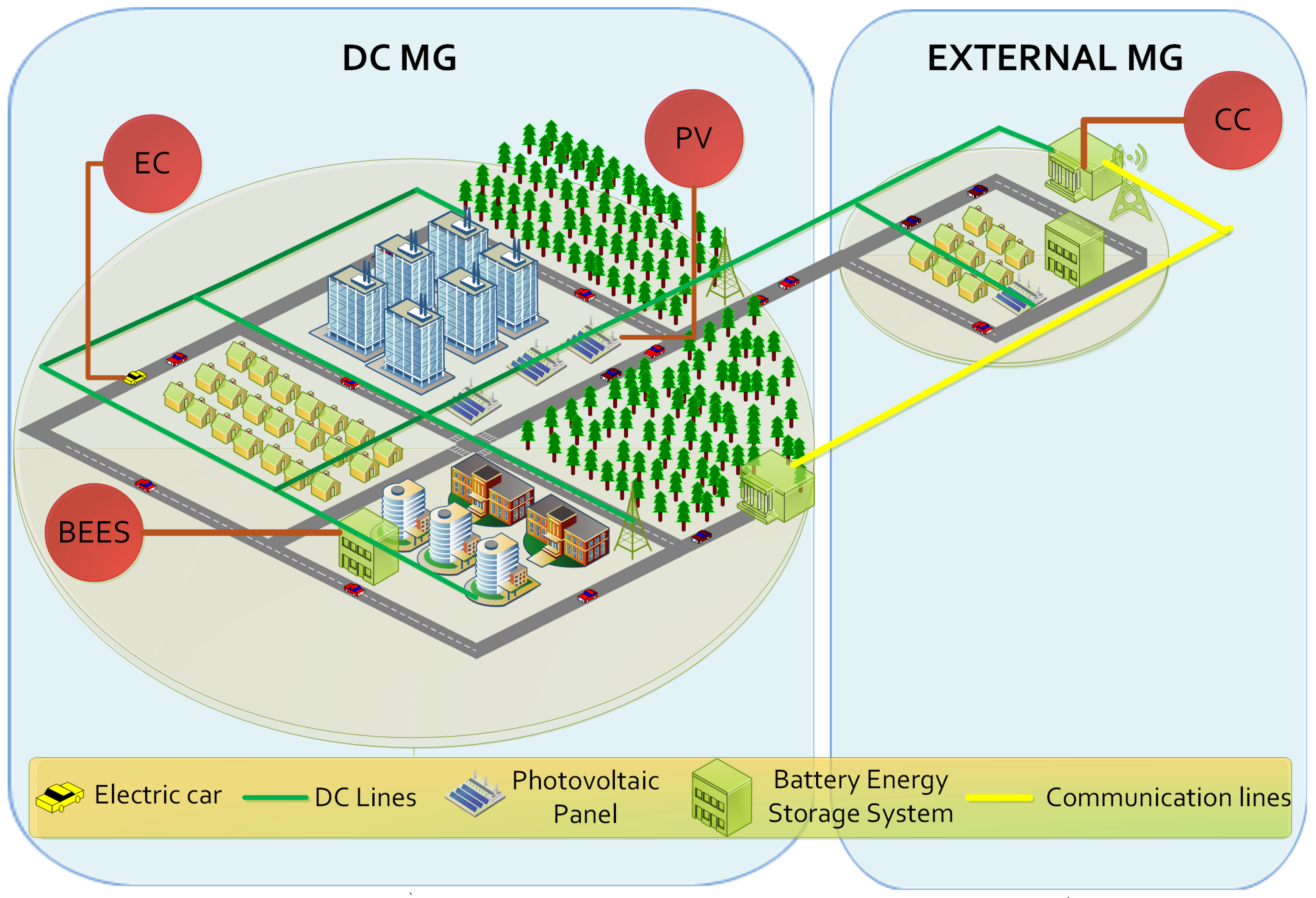
Electrical service in rural areas is limited, and it is necessary to such electrical systems [10]. The RES provides safe and clean electricity that is cheap and more accessible for people who are living with no access to electricity [11,12,13]. Several MG configurations have different features, each presenting advantages and drawbacks depending on the application [14]. Figure 1 shows a DC MG structure, where there are elements such as electric cars, photovoltaic (PV) generators, ESS, DC electrical connections and communication lines. In the same figure, the DC MG connects to an external MG, and their actions are coordinated through shared electrical variables [15].

Recent research proposes new control techniques that implement more robust strategies and use forecast capacities to mitigate errors or disturbances [16,17,18,19]. In addition, MG also has RES, which is purely dynamic, and has some uncertainties and non-linear behavior for certain operating conditions [20,21]. Thus, new control methods are proposed, for example, a distributed predictive control, which improves the power grid robustness, and increases system reliability and predicts possible failures in the system [22,23].

Stochastic models have been considered in [24,25]. These papers proposed to incorporate of typical environment uncertainties, and they integrated an optimal scheduling tool, which had a positive impact in the reduction of carbon emissions and in the increasing of energy efficiency.

The study [26] proposed two different strategies for predictive control. The first was a model predictive control (MPC) based on proportional integral (PI) control. MPC controllers have the advantage of reflecting the intermittent nature of RES [27]. The paper [28] explores an MG optimization procedure with mixed-integer linear programming reducing the computational cost in the classical approach, while [29] details the procedure to satisfy a demand power with maximum utilization of renewable resources using an energy management system.

The paper has feasible results, because there is a significant improvement in the MG response when compared with traditional control techniques. The main contributions of this research are the implementation of a control, which is highly robust and is not susceptible to disturbances typical of an MG. The proposed strategy implements MPC, which improves the point of common coupling (PCC) voltage. As result, the system has better parameters for maximum peak (MP) overshoot and settling time (ts). If the MP obtained in [30] is analyzed, it can be seen that it is around 18% while in our research it is less than 5%, although different methodologies were used for the control, the effect of having a predictive control is better. In the research developed in [31], when injecting a disturbance in the MG, the general control takes around 0.05 s to stabilize the voltage, while in our research the time is around 0.01 s; although they are not exactly similar scenarios, the proposed methodology is superior in terms of robustness.

The document is organized as follows: Section 2 shows the applied methodology. Section 3 describes the discussion and analysis. Finally, conclusions and future works are in Section 4.

2. Methodology

This research proposes a control strategy for DC MG using MPC, which is highly robust and is not susceptible to disturbances typical of this kind of system. In this section, the general control methodology used in the coordination of controllers for the improvement of voltage stabilization is described. Figure 2 shows the proposed strategy. In this, the MPC performs system identification in the block G, which is done using the inputs and output measurement data.

Many methods have been implemented to identify the converters, such as modeling by data acquisition [32,33] or by means of averaged differential equations [34]. The research work developed by [35] allows us to obtain a fairly approximate modeling of the different converters. This research began by analyzing the state space of the switches converter, in active—Equations (1) to (2)—and inactive states—Equations (3) to (4). Then, the state space average model is shown in Equations (5)–(7). Finally, average model of the final state space is in Equations (8) and (9).

$$\dot{x}=A_1\ast x+b_1\ast V_g$$

(1)

$${\mathit{y}}_1=C_1^T\ast x$$

(2)

$$\dot{x}=A_2\ast x+b_2\ast V_g$$

(3)

$${\mathit{y}}_2=C_2^T\ast x$$

(4)

$$\mathit{A}=d\ast A_1+d^{\prime }\ast A_2$$

(5)

$$\mathit{b}=d\ast b_1+d^{\prime }\ast b_2$$

(6)

$${\mathit{c}}^T=d\ast c_1^T+d^{\prime }\ast c_2^T$$

(7)

$$\dot{\widehat{x}}=A\ast x+b\ast \widehat{V_g}+[(A_1-A_2)\ast x+(b_1-b_2)\ast V_g]\ast \widehat{d}$$

(8)

$$\widehat{y}=C^T\ast x+(C_1^T-C_2^T)\ast x\ast \widehat{d}$$

(9)

As reviewed in [36], a transfer function can be taken into state space and vice versa. For the bidirectional converter, the transfer function $G_A$ has the buck converter behavior in Equation (10) and $G_B$ has the boost converter behavior in Equation (11). The converter will only act as a boost or buck converter, but not both at the same time.

$${\mathit{G}}_A=\frac{V_s}{L\ast C\ast (s^2+\frac{s}{R\ast C}+\frac{1}{L\ast C})}$$

(10)

$${\mathit{G}}_B=-\frac{V_o}{R\ast C\ast (1-D)}\ast \frac{\frac{s\ast L-R\ast {(1-D)}^2}{L}}{s^2+\frac{s}{R\ast C}+\frac{{(1-D)}^2}{L\ast C}}$$

(11)

In [37], the pole assignment method is described. For the application of this method, the controller poles are located in a specific location, in order for the output system response to act as the intended response. The controllers are proportional (P), proportional integral (PI) and proportional integral derivative (PID), which will assign 1, 2 and 3 poles, respectively. For the description of the method, the Equation (12) is second-order plant system, while the PID controller is in Equation (13) and the characteristic equation for the closed-loop system 1 + $G_p$*$G_c$= 0, which is algebraically expressed in Equation (14). Therefore, considering the response of the system with a PID control, the characteristic equation will be Equation (15). Finally, equating coefficients of the polynomials expressions (14) and (15) produces Equations (16)–(18).

$${\mathit{G}}_p\left(s\right)=\frac{K_p}{(1+s\ast T_1)(1+s\ast T_2)}$$

(12)

$${\mathit{G}}_c\left(s\right)=\frac{K(1+s\ast T_i+s^2\ast T_i\ast T_d)}{s\ast T_i}$$

(13)

$${\mathit{s}}^3+s^2\left(\frac{1}{T_i}+\frac{1}{T_2}+\frac{K_p\ast K\ast T_d}{T_1\ast T_2}\right)+s\left(\frac{1}{T_1\ast T_2}+\frac{K_p\ast K}{T_1\ast T_2}\right)+\frac{K_p\ast K}{T_1\ast T_2}=0$$

(14)

$$(s+\alpha )(s^2+2\ast ϵ\ast {\omega }_n\ast s+{\omega }_n^2)=0$$

(15)

$$\mathit{K}=\frac{T_1\ast T_2\ast (2\ast ϵ\ast {\omega }_n+\alpha )+1}{K_p}$$

(16)

$${\mathit{T}}_i=\frac{K_p\ast K}{T_1\ast T_2\ast {\omega }_n^2\ast \alpha }$$

(17)

$${\mathit{T}}_d=\frac{T_1\ast T_2\ast {\omega }_n^3\ast \alpha \ast ({\omega }_n+2\ast ϵ\ast \alpha )}{T_1\ast T_2\ast (2\ast ϵ\ast {\omega }_n+\alpha )-1+T_1\ast {\omega }_n^2\ast \alpha \ast ({\omega }_n^2\ast \alpha +1)}$$

(18)

The new processes implemented in the different fields of industry require new optimal control strategies. The Ziegler and Nichols method (Z&N) is a classical method for optimal controller tuning. It is quite efficient for driving DC converters by obtaining an efficient response, which is in the transient state and high performance in its fstability [38]. According to [39], the method of Z&N and force oscillation methods consist of exciting a system in closed loop with a gain in series, and then altering it from a null value to a critical gain ($K_{cr}$). The critical gain is reached when the system output presents sustained oscillations. At this point, the signal is obtained a signal similar to a sinusoidal, and its period will be known as critical period ($P_{cr}$). It is important to take into account the fact that if the $K_{cr}$ cannot obtained because the system does not present sustained oscillations, the method manifest would be not be applicable.

Table 1. Ziegler and Nichols (Z&N) values for different controllers.

Controller	$K_p$	$T_i$	$T_d$
P	0.5 * $K_{cr}$	∞	0
PI	0.45 * $K_{cr}$	$\frac{1}{1.2}$ * $P_{cr}$	0
PID	0.6 * $K_{cr}$	0.5 * $P_{cr}$	0.125 * $P_{cr}$

contains the rules for different controllers as proposed in the literature.

There is some research in the MPC field, for instance [40,41,42]. The MPC methodology predicts the future system behavior, and it has a wide range of applications, because it solves an optimization problem within a moving time horizon in order to generate future actions for optimal operation of a plant. This research focuses on estimating or predicting the outputs of the system using a mathematical model of the plant. Moreover, this optimization approach develops in a period of time, which is known as prediction horizon. This mathematical methodology requires powerful hardware, because of its computational cost.

An MPC generally determines the control action to optimize the cost function. The cost function describes the desired behavior of the system by comparing the system states model within the MPC with the desired trajectories. The optimization problem is solved in each instantaneous sampling time. It is made for a given horizon to determine the correct control sequence action, taking into account the actual system constraints. At each instantaneous sampling time, only the first control action for the given horizon time is applied to the plant and the rest is ignored. At the next sampling time, the new state measurements for the plant act as the initial condition for the system model and the optimization problem is solved to determine the next control input [43].

Pole assignment is the methodology chose the controller, and the procedure is quite clear and it is described in [44]. The controller changes the behavior of the buck converter transfer function, and the PID controller characteristic Equation (19). Meanwhile, the pole assignment method implements the characteristic Equation (20). The controller’s gains $K_p$, $T_d$ and $T_i$ are in the Equations (21)–(23), respectively, which are the result of operating the Equations (19) and (20).

$${\mathit{s}}^3+s^2\left(\frac{1}{R\ast C}+K_P\ast T_d\frac{V_s}{L\ast C}\right)+s\left(\frac{1}{L\ast C}+K_p\frac{V_s}{L\ast C}\right)+\frac{K_p\ast V_S}{L\ast C\ast T_i}=0$$

(19)

$${\mathit{s}}^3+s^2(2\ast ϵ\ast {\omega }_n+\alpha )+s({\omega }_n^2+2\ast \alpha \ast ϵ\ast {\omega }_n)+\alpha \ast {\omega }_n^2=0$$

(20)

$${\mathit{K}}_p=({\omega }_n^2+2\ast \alpha \ast ϵ\ast {\omega }_n)\frac{L\ast C}{V_s}-\frac{1}{V_s}$$

(21)

$${\mathit{T}}_d=\left(2\ast ϵ\ast {\omega }_n+\alpha -\frac{1}{R\ast C}\right)\frac{L\ast C}{K_p\ast V_s}$$

(22)

$${\mathit{T}}_i=\frac{K_p\ast V_s}{L\ast C\ast \alpha \ast {\omega }_n^2}$$

(23)

The iterative algorithm to find the PID controller coefficients for the buck converter is Algorithm 1. The $ϵ$ calculation is based on MP, and ${\omega }_n$ on ts. Next, the pole location $\alpha$ is calculated based on the while loop, which ends when the minimum error is reached. The natural frequency and damping coefficient will be calculated through the equations already known for second-order systems. Additionally, the error refers to the subtraction between the required overshoot and the obtained by the algorithm.

Algorithm 1 Algorithm PID buck converter.

Require:   Input L, C, R, D, $V_s$, setpoint, MP, $t_s$, p(TF buck). 1: $ϵ\leftarrow \frac{-log\left(\frac{MP}{100}\right)}{\sqrt{{\pi }^2+log{\left(\frac{MP}{100}\right)}^2}}$ 2: $\omega n\leftarrow \frac{4}{ϵ\ast tss}$ 3: while$error>0.1$do 4:     $ϵ\leftarrow \frac{-log\left(\frac{MP}{100}\right)}{\sqrt{{\pi }^2+log{\left(\frac{MP}{100}\right)}^2}}$ 5:     ${\mathit{K}}_p\leftarrow ({\omega }_n^2+2\ast \alpha \ast ϵ\ast {\omega }_n)\frac{L\ast C}{V_s}-\frac{1}{V_s}$ 6:     ${\mathit{T}}_d\leftarrow (2\ast ϵ\ast {\omega }_n+\alpha )\frac{L\ast C}{K_p\ast V_s}$ 7:     ${\mathit{T}}_i\leftarrow \frac{K_p\ast V_s}{L\ast C\ast \alpha \ast {\omega }_n^2}$ 8:     $\mathit{c}\leftarrow ftcontroller$ 9:     $\mathit{cl}\leftarrow feedback(c,p)$ 10:     $\mathit{y}\leftarrow response(cl,t)$ 11:     for x=1:length(t) do 12:         $\mathit{matriz}(\mathit{m},:)\leftarrow \left[y\right(x)$$t\left(x\right)]$ 13:     $\mathit{mayor}\leftarrow firstelementmatrix$ 14:     for x=1:lenght(t) do 15:         if matriz(x,1)≥ max then 16:            $\mathit{max}\leftarrow findmax$ 17:     $\mathit{error}\leftarrow abs(SP-MP)$ 18:     $\mathit{alpha}\leftarrow alpha+100$ 19: $\mathit{step}(\mathit{setpoint}\ast \mathit{lc},\mathit{t})$

If sustained oscillations with a period $P_{cr}$ are reached, the $K_{cr}$ is the critical controller gain. In addition, the ZN method can be determined, but sometimes it is not feasible. In the work done by [44], an analytical procedure is developed to determine these constants, which have been simplified in this article. The TF and gain margin in closed-loop are in the Equation (24), which has 1 zero and 2 poles.

$${\mathit{G}}_{LC}\left(s\right)=\frac{K_p\ast G_p}{1+K_p\ast G_p}$$

(24)

The use of the Routh–Hurthwitz (RH) criterion allows us to find the critical gain, which the system oscillates. This methodology uses the parameter D in Equation (25), and a summary of RH criterion, depending on the controller type as presented in

Table 2. Routh–Hutwitz analysis.

$s^2$	1	$\frac{{(1-D)}^2}{L\ast C}-K_p\frac{-V_o\ast R{(1-D)}^2}{R\ast C(1-D)L}$
s	$\frac{1}{R\ast C}+K_p\frac{-V_o}{R\ast C(1-D)}$
$s^0$	$\frac{{(1-D)}^2}{L\ast C}-K_p\frac{-V_o}{R\ast C(1-D)}\frac{R\ast {(1-D)}^2}{L}$

. Thus, the critical gain is obtained from Equation (26). Nevertheless, this gain formula is a standard for the converter designing processes for determining the consisted oscillations. if the identification and control techniques proposed are used, an even more similar analysis could be made to determine the controller in any plant that has similar characteristics to the TF [45].

$${\mathit{s}}^2+s\left(\frac{1}{R\ast C}+K_p\frac{-V_o}{R\ast C(1-D)}\right)+\left(\frac{{(1-D)}^2}{L\ast C}-K_p\frac{-V_o}{R\ast C(1-D)}\frac{R{(1-D)}^2}{L}\right)=0$$

(25)

$${\mathit{K}}_{cri}=\frac{1-D}{V_o}$$

(26)

In the same way, the oscillation period can be found from the analysis of Equation (27), taking it to the j$\omega$, while the critical frequency and period can be obtained by equating the real terms of Equations (28)–(30).

$${\left(jw\right)}^2+\left(jw\right)(\frac{1}{RC}+K_p\frac{-V_o}{RC(1-D)})+(\frac{{(1-D)}^2}{LC}-K_p\frac{-V_o}{RC(1-D)}\frac{R{(1-D)}^2}{L})=0$$

(27)

$$-w^2+jw(\frac{1}{RC}+\frac{1-D}{V_o}\frac{-V_o}{RC(1-D)})+(\frac{{(1-D)}^2}{LC}-\frac{1-D}{V_o}\frac{-V_o}{RC(1-D)}\frac{R{(1-D)}^2}{L})=0$$

(28)

$${\mathit{w}}_{cri}=\sqrt{2\frac{{(1-D)}^2}{LC}}$$

(29)

$${\mathit{P}}_{cri}=\frac{2\pi }{w_{cri}}=\frac{2\pi }{\sqrt{2\frac{{(1-D)}^2}{LC}}}$$

(30)

The pseudo-code in Algorithm 2 determines the Z&N method, which calculates the critical factors for each type of controller. Thus, the equations calculate the critical factors and they corroborate the behavior of sustained oscillations in the output system. Thereby, the critical controller gains are obtained by means of the Z&N tuning technique. The plant output response fulfills the design conditions, with the Z&N calculated gains. The proposed method specifies that these gains can be minimally deviated to achieve a better response; thus, an increase in the PID gains is incorporated in the pseudo-code. As a result, when using the adjusted Z&N controller the plant has less overshoot and higher damping coefficient.

Algorithm 2 PID boost parameters assigment using critical gain and period

Require:  Input L, C, R, D, $V_s$, setpoint, p(TF boost). 1: $\mathit{K}cri\leftarrow \frac{1-D}{V_o}$ 2: $\mathit{P}cri\leftarrow \frac{2\pi }{\sqrt{\frac{2{(1-D)}^2}{L\ast C}}}$ 3: $\mathit{K}p\leftarrow 0.6\ast Kcri$ 4: $\mathit{T}i\leftarrow 0.5\ast Pcri$ 5: $\mathit{T}d\leftarrow 0.125\ast Pcri$ 6: $\mathit{K}p\leftarrow Kp+0.003$ 7: $\mathit{T}i\leftarrow Ti+0.0001$ 8: $\mathit{T}d\leftarrow Td+0.0005$ 9: $\mathit{c}\leftarrow ftcontrolador$               ▹ Calculate it 10: $\mathit{cl}\leftarrow feedback(c\ast p,1)$ 11: $\mathit{y}\leftarrow step(setpoint\ast lc,t)$ 12: $\mathit{step}(\mathit{setpoint}\ast \mathit{lc},\mathit{t})$

3. Analysis and Discussion

The MG controllers coordination strategy governs locally through a continuous supervision of generated power, and to control the PCC voltage. Thus, the power feeders integration to the electrical network allows us to maintain a stable voltage within the design limits, and it provides the activation signals of the electronic circuit breakers. Meanwhile, the controller is based on model predictive control (MPC) and its training parameters are summarized in

Table 3. MPC training parameters.

Parameter	Value
Sample time	0.05 $\mathsf{\mu }$s
Prediction horizon	10
Control horizon	2

. The inputs to the MPC block are the voltage reference, the feedback output signal (mo) and the system disturbances, D and E. The system output (YMPC) is compared with the PCC voltage, which is the deviation signal (e). The signal e and the real-time measurement of the Power (P) are the inputs for the overall system.

The evaluation parameter for the settling time (ts) is 0.2 s, and maximum overshoot (MP) percentage is 10%. Furthermore,

Table 4. DC microgrid design criteria.

Parameters	Symbols	Value	Units
Sample time	T	0.5 $\times {10}^{-6}$	s
Switching frequency	$fc$	25	KHz
PCC Voltage	$V_o$	300	v
Voltage ripple	$\Delta V_o/V_o$	1	%
Settling time	$t_s$	0.2	s
Maximum overshoot	MP	10	%

shows the design criteria for the DC microgrid [1,46]. Meanwhile, the sampling time measurement is 0.5 $\mathsf{\mu }$s, which is less than the switching period. However, the switching frequency is 25 KHz, because it is above the human audible frequency range. The output voltage ripple depends on the chosen filter and the PCC voltage, which is 300 volts, has been chosen according to [3].

For the control validation, a set of dynamic loads are connected to the system, which is gradually incorporated throughout the simulation time, whether these disturbances are characteristic of the plant dynamics or depend on external factors. There are two modes of operation. The first is the minimum demand scenario, where five loads are gradually fed, at the beginning of the study, when power is supplied to a 3.6 kW load and to two buck converters.

Table 5. Power supplied.

N	Power (Kw)	Time (s)
1	7.44	0.0
2	11.04	0.05
3	14.64	0.07
4	18.24	0.09
5	21.84	0.11
6	36.24	0.13

shows the experiment parameters. The second is the maximum demand scenario, where all loads are incorporated to the MG, and in the last switching there is an increase of 14.4 kW in the power demanded by the subscribers.

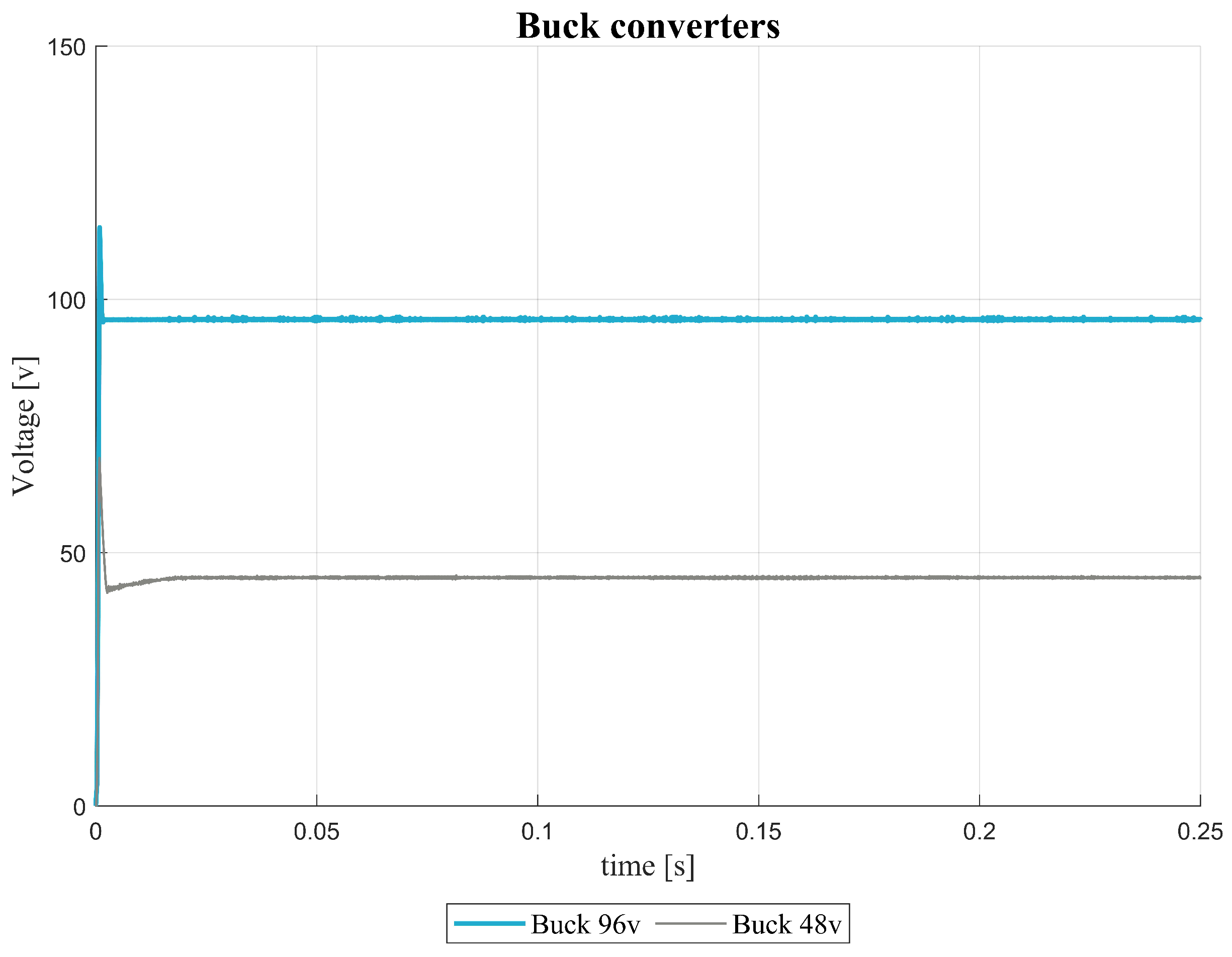
The network configuration has two different voltage outputs regulated by each buck converter at 96 and 48 volts, respectively. Here, the input is PCC voltage, while the output responses are under-damped as can be reviewed in Figure 3, and the main design parameters, such as MP and $t_s$, are reached by the controller.

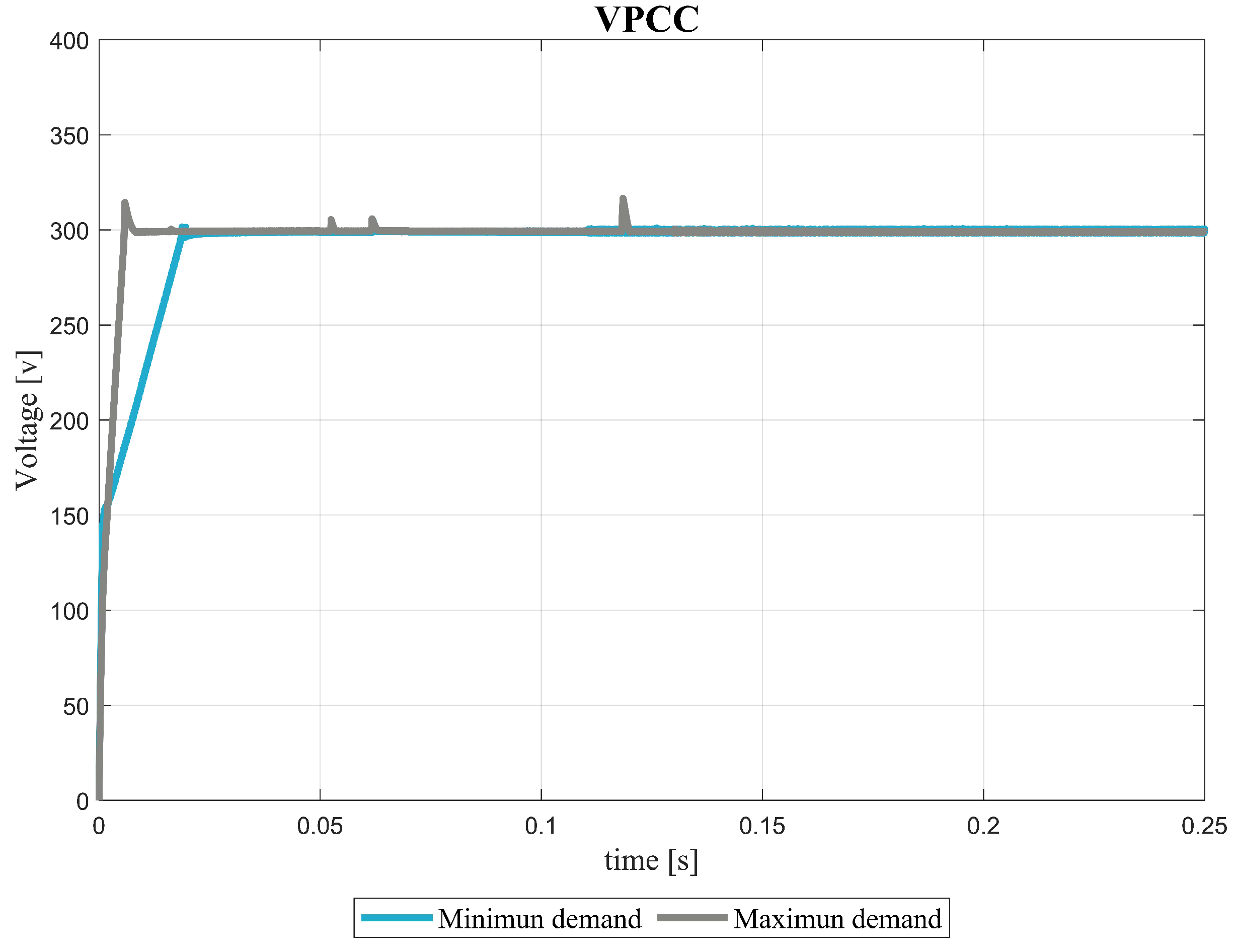
Figure 4 shows the PCC voltage response in minimum and maximum demand cases, and the MG control is especially focused on this parameter since it will allow validation of the design criteria. Moreover, the PCC voltage is responsible for supplying the voltage to the subscribers. It can be seen that the voltage has a similar response to an under-damped system. However, it will reach a minimum MP percentage, but at the cost of having a slower system response. Nevertheless, the control design was made so that there is a balance between the MP and $t_s$.

The parameters are summarized in

Table 6. Resulting system parameters in the output system.

Parameter	Symbol	Value	Units
Voltage ripple	$\Delta V_o/V_o$	0.1	%
PCC voltage	$V_o$	300	v
Settling time	$t_s$	0.012	s
maximum overshoot	MP	4.8	%

, which are obtained in the PCC voltage response. The voltage is around the desired values, and the voltage ripple is 0.1%, the settling time is 0.012 s and the MP is 4.8%. As a result, those resulting parameters are lower than those proposed in Table 4. However, the obtained result from the disturbance injection experimentation shows peaks from the effect of variations in the load and the selective load connection in the system. Those peaks do not exceed the proposed MP, and the system is rapidly restored to 300 voltage.

Table 7. Connection and disconnection for power supplies in minimum demand.

Interval [s]	S1	S2	S3	S4	ES
0–0.5	1	1	0	1	0
0.5–0.8	1	1	1	1	0
0.8–0.11	1	1	1	1	0
0.11–0.13	1	1	1	1	0
0.13–0.25	1	1	1	1	0

and

Table 8. Connection and disconnection for power supplies in maximum demand.

Interval [s]	S1	S2	S3	S4	ES
0–0.5	1	0	0	1	0
0.5–0.8	1	1	0	1	0
0.8–0.11	1	1	1	1	0
0.11–0.13	1	1	1	1	1
0.13–0.25	1	1	1	1	1

summarize the connection of each of the power supplies (S) and the external supply (ES) in the two possible scenarios, i.e., in minimum and maximum demand, while the time intervals is similar to those of the dynamic loads switching. When the supply is represented by the number 1, it means that the supply is connected, and the number 0 indicates when it is disconnected. It is worth knowing that for a bidirectional power supply, it may or may not deliver power depending on the control strategy. On the one hand, in minimum demand scenario, the S1 and S2 deliver energy, while S3 and ES are not activated, because the power delivered to load is sufficient, and S4 is activated for all time because in this scenario it receives energy. On the other hand, in maximum demand scenario, S1 and S4 deliver power, and they are activated for the whole simulation period, since power must always be available at the PCC. Meanwhile, S2 and S3 are incorporated to the MG according to the demanded power. In addition, finally, the ES, which is an external MG source, would be incorporated if the local supply is not sufficient.

Figure 5 describes the instantaneous power for minimum demand scenario. First, there is a power supplied balance in each converter when there are no load additions. Second, due to the proposed control strategy, the S4 power is negative, because it receives energy. It should be noted that the power suppliers have this behavior because it depends on the demanded power fluctuations and the converters’ incorporation, which occurs in different lapses of the period. Figure 6 describes the instantaneous power generated by each energy source in the maximum demand scenario. It provides meaningful information: the supply loads activate in the period from 0.05 to 0.13 seconds.

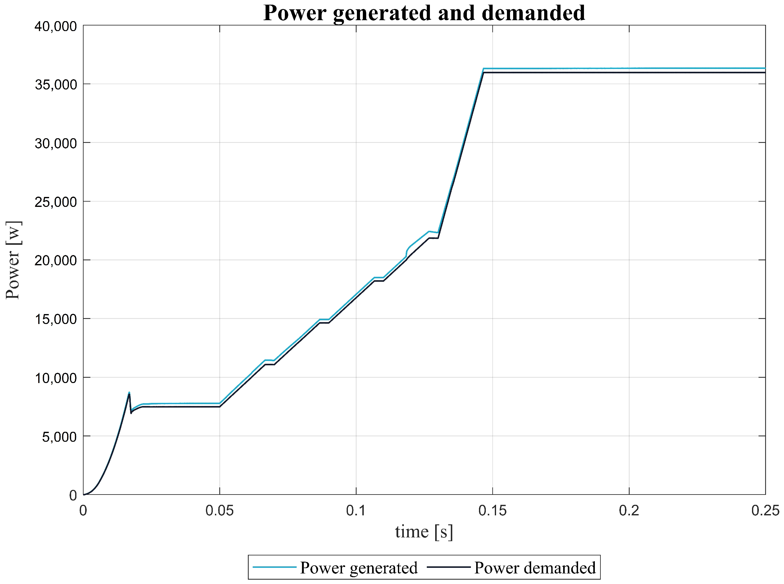
Figure 7 describes the average generated and demanded power. Initially, the power generation presents a peak in 0.02 s, which results from the connection of whole subscribers, but then the power flow stabilizes. It is remarkable to see the existing ramps in the simulation period, which are product of the loads incorporation in the MG.

In this context, there are certain circumstances in which power generation is compromised and, as a consequence, there is a significant power reduction. Environment conditions are one the most important factors, either due to changes in climatic conditions, such as radiation, temperature, and due to the subscribers growing. If there is a reduction in power, the general control behavior would be affected. As long as the predictive control has an internally predefined model it could have serious failures in the voltage stabilization in the electrical system [47].

Figure 8 describes a brief comparison of two types of controls implemented in MG. On the one hand, the system response with MPC controller response is highly robust, where the MP is initially less than 10%, and the ts is less than 0.2 s. The observed peaks voltages, in certain time intervals, are due to the subscribers integration. As a result, the MPC controller copes the system disturbances, and even allows us to obtain a voltage ripple of around 0.5%. On the other hand, the classical PI control MG response presents a ts similar to the MPC approach. However, the controller tries to establish the voltage around 300 v, but there are certain fluctuations around the reference until it settles down after 0.05 s. Finally, the system tends to become unstable and even maintains a voltage ripple around 17%, when the last load is incorporated.

4. Conclusions and Future Works

In this research paper, a direct current microgrid was implemented, which was focused on the rapid stabilization of the point of common coupling voltage and on the rejection of the disturbances. The simulation results obtained satisfy the proposed design guidelines by obtaining a maximum overshoot of 4.8%, settling time of 0.012 s and a voltage ripple of 0.1%.

Individual controllers were implemented for each power supply through the iterative algorithms development, emphasizing local and then general control, although the response for minimum demand is relatively slow compared to maximum demand. In both scenarios the design criteria are met.

A control strategy combining classical, model predictive control and logic control was implemented, focusing as inputs the instantaneous parameters of the point of common coupling voltage and the system active power for coupling and decoupling to the microgrid. This strategy reached the system energy balance without affecting the voltage stabilization, however, in the case of bidirectional converters, positive power graphs are obtained when energy is incorporated to the grid and negative power when the battery banks are in the charging state.

Although the model predictive control is used as a general control, the response of the system to other types of predictive control could be considered in future works. The implementation of a generalized predictive control could be the next step, and it would even allow the evaluation of which type of control is more efficient from the robustness point of view.