Experimental and Co-Simulation Performance Evaluation of an Earth-to-Air Heat Exchanger System Integrated into a Smart Building

Abstract

Building models and their connected subsystems are often simulated as standalone entities. However, in order to monitor a system′s reactions to changing parameters and to assess its energy efficiency, it must be exposed to the actual dynamic context of the building under study. Hence, frameworks assessing co-operative simulation of buildings and their subsystems should be used. In this study, the Building Control Virtual Test Bed (BCVTB) framework was used for co-simulation of a small-scale building (EEBLab) connected to an Earth-to-air heat exchanger (EAHE). The EnergyPlus tool was used to simulate the indoor air temperature variations within the EEBLab, and MATLAB was used to model the EAHE system and to calculate its performance based on various parameters. The HOLSYS internet of things platform was deployed to monitor and collect the experimental data from the sensors to validate the simulations. A favorable agreement between the experimental and simulation results was obtained, showing the contribution of the small-scale EAHE system in maintaining a comfortable indoor temperature range inside EEBLab. Moreover, it demonstrated the effectiveness and accuracy of the proposed approach for integrated building co-simulation and performance evaluation.

1. Introduction

Attaining clean energy transition demands colossal efforts. Hence, when talking about energy efficient buildings, it is important to highlight the perplex structures made from different yet connected entities that interact together in the most unpredictable ways. These entities are mainly represented in our holistic approach as a pyramid (see Figure 1), made of three main stratified layers: the envelope, the integrated passive/active systems, and the integrated renewable energy sources and storage devices, as well as control strategies depicted by an external fourth layer to communicate all the layers together. In other words, multiple coexisting aspects of a building have to be controlled in a holistic way to ensure occupant comfort while decreasing energy consumption. This integrated approach requires supporting tools. Recently, cooperative simulations were proposed in order to allow submodels of different systems to communicate by exchanging data in response to a certain defined time step. For this, multiple frameworks were developed and are in use (e.g., BCVTB).

In this paper, we main focusing on the exploitation of geothermal energy by integrating an Earth-to-air heat exchanger (EAHE) prototype into a small prefabricated building. This technology is known to be promising for preheating the air in winter and for precooling it in summer to ensure inside-zone thermal comfort. Fresh air circulates through the buried pipes and exchanges air with the ground/soil temperature. During summer, the air is cooled while passing inside the pipes (following the first law of thermodynamics), minimizing the cooling demand. In winter, the process is reversed as the ground maintains its temperature throughout the year [1]. The main objective is to evaluate its performance as well as its effectiveness in reducing energy consumption and maintaining occupant thermal comfort in response to real dynamics of the considered building, while deploying the BCVTB platform

The work presented in this paper is an extension of the work communicated in [2] and is part of an ongoing project named HOLSYS, funded by the Moroccan Research Institute for Solar Energy and New Energies (IRESEN). The HOLSYS project’s main objective is to study the impact of the use of information and communication technologies (ICT) and their solutions on occupants’ comfort, bills and energy savings in smart buildings, including extracting relevant information from streaming data (e.g., electricity consumption) in order to increase occupant awareness. The aim is to control, either manually or automatically, the usage of high energy-consuming appliances according to the produced energy. We are mainly investigating the effectiveness of automatic systems and RES integration for energy saving and occupant satisfaction. In summary, the contribution of this work is two-fold: (i) performance evaluation of the EAHE system as a renewable energy source and (ii) showing the importance of the cooperative approach in evaluating the building performances as a complex system, including its linked equipment.

2. Related Work

Energy-efficient buildings are made from various entities that constantly interact with each other. These entities are mainly represented as the envelope of the building, the connected systems to it (active, passive, renewable energy sources), occupant behavior, and means of control. The envelope, it represents the pillar of every sufficient and efficient building. Hence, we usually tend to perform simulations in order to examine the construction materials and the geometry of the building in general before moving to the actual building-up phase. For this, various simulation methods, models and tools are introduced and then widely used. For instance, Bhamare et al. [3] presented, using ANSYS fluent in combination of a user-defined function using C++, a full-scale 3D numerical model of a building in order to evaluate the effect of integrating phase change materials on heat transfer and thermal comfort. Berrabah et al. [4] generated a thermal and mechanical model of a small-scale laboratory using the finite element method under the Cast3m tool. The developed model was validated against experimentation using numerical sensors and thermography analysis.

It was also shown by diverse studies that buildings usually consume the most while they are operating, due to the heavy usage of HVAC and other electric equipment [5]. Consequently, reducing this consumption requires the adoption of passive and active system strategy integration [6].

Integrating passive devices as alternatives to active ones and/or using information and communication technologies (ICT) control approaches may lead to a decrease in energy consumption. However, at times, incorporating these systems to further enhance occupant comfort may lead to an increase in energy consumption. For this, it is strongly recommended to use renewable energy sources (RESs) as alternatives, in parallel with adequate storage devices. When discussing RESs, we can mention solar, thermal, wind, hydroelectric as well as geothermal energy. For instance, the latter has been widely used for reducing ventilation heat losses while enhancing thermal comfort in buildings [7]. It mainly works on exploiting the ground’s internal temperature to heat or cool with heat circulating through the installation pipes. Researchers have given it much attention during the last decades in terms of modeling, sizing and deploying similar systems, since it is an approximately cheap and efficient alternative to conventional energy. For instance, Sodha et al. [8] found the ground temperature distribution using Fourier’s coefficient calculation including that this temperature fluctuates randomly in response to the atmospheric temperature variation. However, this variation decreases with depth to become a small constant at about 4 mf. Bisonya et al. [9] gave an extensive literature review on the experimental and analytical studies of EAHE systems, covering their characteristics and models as well as their designs. Tiwari et al. presented in [10] a model of an EAHE that they designed in response to ground characteristics and external weather conditions as well as room dimensions. Bowen et al. [11] presented the concept of indirect coupling to heat and cool the air inside a building using an Earth–air tunnel system. Touzani et al. [12] presented an experimental study on a Canadian well, which was installed under a villa in Rabat. Performances of the system were evaluated through the seasons. Moummi et al. [13] proposed an analytical model of air temperature evolution. This model is beneficial for sizing an EAHE when experimental data are not available.

Integrating all these active, passive systems and renewable energy sources to enhance energy efficiency in buildings is becoming primordial. However, before moving on to the execution phase, it is important to evaluate them through the usage of simulation tools. These tools are usually conceived to model each subsystem on its own, not capturing all the dynamic of a building and its integrated components. For this, cooperative simulation has received much attention in the last few years. Co-simulation allows each of the submodels of the systems to be realized in its own particular simulation environment, using a specified model description. Meanwhile, subsystems implicitly exchange data as a means of communication. Schloegl et al. suggested in [14] a classification scheme for co-simulation approaches in energy systems. The main objective is to facilitate communication between the users and developers and to help define the most suitable tool for any simulation purposes. Bleicher et al. [15] presented in their work a co-simulation environment for optimizing energy efficiency in production processes in order to assure economic competitiveness in the early planning phases. Welsch et al. [16] developed a TCP/IP interface allowing for the coupling of the MATLAB-SIMULINK software to the FEFLOW finite element program. It was shown that small communication time steps are able to reduce data exchange errors between simulators and make the coupling more robust and reliable. Cellura et al. [17] proposed a co-simulation approach integrating the building simulation and life cycle assessment. This was achieved by programming a TRNSYS component performing cradle-to-cradle life cycle assessment studies. Cucca et al. [18] developed a co-simulation tool coupling both Dymola–Modelica for energy systems and EnergyPlus building simulations. Communication between simulators had been processed using a FMU block providing, to Dymola, weather data, building heat demand and photovoltaic power production. Three scenarios were studied, and they proved that the developed tool is able to implement and evaluate various control strategies in buildings. Yao presented in [19] a co-simulation model linking the EnergyPlus building model to manually controlled solar shade models made under the BCVTB framework. The main purpose is to define the impact of control behavior of solar shading devices on the energy performance of buildings.

The work presented in this paper focuses on the development of an integrated approach toward efficient and holistic buildings simulations. The BCVTB co-simulation framework was used to simulate a small-scale building linked to an Earth-to-air heat exchanger system. Each subsystem was modeled and validated experimentally before integrating them for co-simulation and integrated performance evaluation.

3. Mathematical Modeling

3.1. Building Description and Modeling

The considered specimen is a set of two small-scaled prefabricated buildings based at the International University of Rabat (see Figure 2). It is mostly used to conduct research activities (materials of construction and insulation, integration of renewable energy sources, ICT for smart control and data collection, etc.) and is sometimes used as an office. A single prefabricated building accounts for 12 m² of surface and 30 m³ of volume. It is mainly made of galvanized steel and an integrated foam polyurethane insulation in its lateral walls. As for the roof, it is made of galvanized steel, an air gap, and plaster. Finally, the flooring is made from galvanized steel and internal chipboard. The building is southeast oriented and contains one single-glazed window and a door on its south facade. More details about the characteristics of construction materials are presented in

Table 1. Thermal properties of the EEBLab construction materials.

Material	Heat Capacity (J/kg. K)	Density (kg/m3)	Conductivity (W/m. K)
Galvanized steel	470	7800	52
Wood	2100	170	0.042
Plasterboard	1300	25	0.022
Glass	800	2530	0.93
Aluminum	900	2690	210
Polyurethane	1000	40	0.024

.

Real registered data of Sala Al Jadida (latitude: 34.05°, longitude: −6.75°, elevation: 119 m) were taken into account for the simulated period. Figure 3, Figure 4 and Figure 5 represent the external temperature, external solar radiation and internal solar distribution transmitted through the window, respectively. The shapes of the curves demonstrate that external temperature varies between a minimum of 6.48 °C and a maximum of 31.32 °C. This evolution is quite logical given the considered simulated period. As for external solar radiation, its varies following the alternations between day and night and might exceed 829 w/m² at the level of the south facade. Regarding internal solar distribution, the maximum value is in the order of 2.5 w/m² and is distributed almost equally on all facades, except from the west facade, which does not exceed 1.5. As for the ground temperature, it varies from 17.63 °C in December to 16.11 °C in January.

In this section, we aim to evaluate the thermal comfort inside the zone without any ventilation or air conditioning system activated. For this, the simulation was run using the EnergyPlus simulation tool. This tool is a commonly used building simulation program among researchers, engineers and designers. It is considered to be one of the most robust available simulation tools at both the commercial and academic levels. It combines all the entities of a building, starting with the envelope modeling, HVAC systems, passive systems and integrated renewable energy sources. The EnergyPlus program is based on the best capabilities of both DOE-2 and I-Blast simulation programs [20]. Below are the assumptions that we considered during the simulations phase:

• Version: 8.5;
• Load convergence tolerance value: 0.04;
• Temperature convergence tolerance value: 0.4;
• Solar distribution: “Full interior and exterior”;
• Maximum number of warmup days: 25;
• Minimum number of warmup days: 6;
• Surface Convective Algo: Inside: TARP

TARP, or the Thermal Analysis Research Program, blends correlations from AHRAE and flat plate experiments by sparrow et al. [21].

• Surface Convective Algo: Outside: DOE-2.

Combination of MoWitt (measurement taken at the mobile window thermal test facility [22] and BLAST detailed convection models:

• Time step: 6 (calculation each 10 min);
• Site ground temperatures: (values are being set according to experimental data);
• December: 17.63; January: 16.11; February: 16.83;
• Heat balance algorithm: Conduction Transfer Function (CTF);

Heat balance on the zone air is given as follows:

$$C_Z\frac{d{T}_Z}{dt}={\displaystyle \sum }_{i=1}^{Nsl}{\dot{\varphi }}_i+{\displaystyle \sum }_{i=1}^{Nsurf}{h}_i{A}_i\left(T_{s_i}-T_Z\right)+{\displaystyle \sum }_{i=1}^{Nzones}{\dot{m}}_i{C}_p\left(T_{Z_i}-T_Z\right)+{\dot{m}}_{inf}{C}_p\left(T_{\infty }-T_Z\right)+{\dot{\varphi }}_{sys}$$

(1)

$$⟺$$

$${\rho }_{air}{C}_p{C}_T\frac{d{T}_Z}{dt}={\displaystyle \sum }_{i=1}^{Nsl}{\dot{\varphi }}_i+{\displaystyle \sum }_{i=1}^{Nsurf}{h}_i{A}_i\left(T_{s_i}-T_Z\right)+{\displaystyle \sum }_{i=1}^{Nzones}{\dot{m}}_i{C}_p\left(T_{Z_i}-T_Z\right)+{\dot{m}}_{inf}{C}_p\left(T_{\infty }-T_Z\right)+{\dot{m}}_{sys}{C}_p\left(T_{sup}-T_Z\right)$$

(2)

where $C_Z\frac{d{T}_Z}{dt}$ is the energy stored in zone air, ${\displaystyle \sum }_{i=1}^{Nsl}{\dot{\varphi }}_i$ is the convective internal loads, ${\displaystyle \sum }_{i=1}^{Nsurf}{h}_i{A}_i\left(T_{s_i}-T_Z\right)$ is the convective heat transfer from zone surfaces, ${\displaystyle \sum }_{i=1}^{Nzones}{\dot{m}}_i{C}_p\left(T_{Z_i}-T_Z\right)$ is the heat transfer due to interzone air mixing, ${\dot{m}}_{inf}{C}_p\left(T_{\infty }-T_Z\right)$ is the heat transfer due to the infiltration of outside air, ${\dot{m}}_{sys}{C}_p\left(T_{sup}-T_Z\right)$ is the air system output, $h_i$ is the internal heat transfer coefficient, $A_i$ is the surface area, $T_{s_i}$ is the surface temperature, $T_Z$ is the zone temperature, ${\dot{m}}_i$ is the mass flow, ${\dot{m}}_{inf}$ is the infiltration mass flow, ${\dot{m}}_{sys}$ is the system mass flow, $T_{\infty }$ is the ambient infinite temperature, and $C_Z$ is the zone heat capacity, which can include thermal masses assumed to be in equilibrium with the zone air.

In order to solve the heat balance equation, EnergyPlus provides three main algorithms: the 3rdOrderBackwardDifference, the Euler Method, and the analytical solution. The first two methods use the finite difference method, in which the temperature difference is expressed as follows:

$$\frac{dT}{dt}={\left(\delta t\right)}^{-1}\left(T_z^t-T_Z^{t-\delta t}\right)+O\left(\delta t\right)$$

(3)

The Euler formula is mainly used to replace the derivative term of temperature:

$$\begin{array}{cc}\hfill C_Z\frac{T_Z^t-T_Z^{t-\delta t}}{dt}+T_Z^t& \left({\displaystyle \sum }_{i=1}^{Nsurf}{h}_i{A}_i+{\displaystyle \sum }_{i=1}^{Nzones}{\dot{m}}_i{C}_p+{\dot{m}}_{inf}{C}_p+{\dot{m}}_{sys}{C}_p\right)\hfill \\ & ={\displaystyle \sum }_{i=1}^{Nsl}\dot{{\varphi }_i^t}+{\dot{m}}_{sys}{C}_p{T}_{supply}^t\hfill \\ & +{\left({\displaystyle \sum }_{i=1}^{Nsurf}{h}_i{A}_i{T}_{si}+{\displaystyle \sum }_{i=1}^{Nzones}{\dot{m}}_i{C}_p{T}_{Z_i}+{\dot{m}}_{inf}{C}_p{T}_{\infty }\right)}^{t-\delta t}\hfill \end{array}$$

(4)

$$\begin{array}{c}{T}_z^t=\frac{{{\displaystyle \sum }}_{i=1}^{Nsl}\dot{{\varphi }_i^t}+{\dot{m}}_{sys}{C}_p{T}_{supply}^t+}{\frac{C_Z}{\delta t}+\left({{\displaystyle \sum }}_{i=1}^{Nsurf}{h}_i{A}_i+{{\displaystyle \sum }}_{i=1}^{Nzones}{\dot{m}}_i{C}_p+{\dot{m}}_{inf}{C}_p+{\dot{m}}_{sys}{C}_p\right)}\\ +\frac{\left(C_Z\frac{T_Z}{\delta t}+{{\displaystyle \sum }}_{i=1}^{Nsurf}{h}_i{A}_i{T}_{si}+{{\displaystyle \sum }}_{i=1}^{Nzones}{\dot{m}}_i{C}_p{T}_{Z_i}+{\dot{m}}_{inf}{C}_p{T}_{\infty }\right)}{\frac{C_Z}{\delta t}+\left({{\displaystyle \sum }}_{i=1}^{Nsurf}{h}_i{A}_i+{{\displaystyle \sum }}_{i=1}^{Nzones}{\dot{m}}_i{C}_p+{\dot{m}}_{inf}{C}_p+{\dot{m}}_{sys}{C}_p\right)}\end{array}$$

(5)

In order to avoid instabilities, higher-order expressions with corresponding higher-order truncation errors were developed.

$${\frac{d{T}_Z}{dt}|}_t\cong {\left(\delta t\right)}^{-1}\left(\frac{11}{6}{T}_Z^t-3T_Z^{t-\delta t}+\frac{3}{2}{T}_Z^{t-2\delta t}-\frac{1}{2}{T}_Z^{t-3\delta t}\right)+O\left(\delta t\right)$$

(6)

$$\begin{array}{cc}\hfill T_z^t& =\frac{{{\displaystyle \sum }}_{i=1}^{Nsl}\dot{{\varphi }_i^t}+{{\displaystyle \sum }}_{i=1}^{Nsurf}{h}_i{A}_i{T}_{si}}{\left(\frac{11}{6}\right)\frac{C_Z}{\delta t}+\left({{\displaystyle \sum }}_{i=1}^{Nsurf}{h}_i{A}_i+{{\displaystyle \sum }}_{i=1}^{Nzones}{\dot{m}}_i{C}_p+{\dot{m}}_{inf}{C}_p+{\dot{m}}_{sys}{C}_p\right)}\hfill \\ & +\frac{+{{\displaystyle \sum }}_{i=1}^{Nzones}{\dot{m}}_i{C}_p{T}_{Z_i}+{\dot{m}}_{inf}{C}_p{T}_{\infty }+{\dot{m}}_{sys}{C}_p{T}_{supply}^t}{\left(\frac{11}{6}\right)\frac{C_Z}{\delta t}+\left({{\displaystyle \sum }}_{i=1}^{Nsurf}{h}_i{A}_i+{{\displaystyle \sum }}_{i=1}^{Nzones}{\dot{m}}_i{C}_p+{\dot{m}}_{inf}{C}_p+{\dot{m}}_{sys}{C}_p\right)}\hfill \\ & -\frac{-\left(\frac{C_Z}{\delta t}\right)\left(\frac{11}{6}{T}_Z^t-3T_Z^{t-\delta t}+\frac{3}{2}{T}_Z^{t-2\delta t}-\frac{1}{2}{T}_Z^{t-3\delta t}\right)}{\left(\frac{11}{6}\right)\frac{C_Z}{\delta t}+\left({{\displaystyle \sum }}_{i=1}^{Nsurf}{h}_i{A}_i+{{\displaystyle \sum }}_{i=1}^{Nzones}{\dot{m}}_i{C}_p+{\dot{m}}_{inf}{C}_p+{\dot{m}}_{sys}{C}_p\right)}\hfill \end{array}$$

(7)

The major problem with this 3rdOrderBackwardDifference resolution method is that it has truncation errors and requires a fixed time step length for the first three time steps. For this, an analytical resolution was developed to obtain solutions without truncation errors and is independent of time step length. The temperature of the considered zone is then expressed as follows:

$$\begin{array}{cc}\hfill T_Z^t& =(T_Z^{t-\delta t}-\frac{{{\displaystyle \sum }}_{i=1}^{Nsl}\dot{{\varphi }_i^t}+{{\displaystyle \sum }}_{i=1}^{Nsurf}{h}_i{A}_i{T}_{si}+{{\displaystyle \sum }}_{i=1}^{Nzones}{\dot{m}}_i{C}_p{T}_{Z_i}}{{{\displaystyle \sum }}_{i=1}^{Nsurf}{h}_i{A}_i+{{\displaystyle \sum }}_{i=1}^{Nzones}{\dot{m}}_i{C}_p+{\dot{m}}_{inf}{C}_p+{\dot{m}}_{sys}{C}_p}\hfill \\ & +\frac{+{\dot{m}}_{inf}{C}_p{T}_{\infty }+{\dot{m}}_{sys}{C}_p{T}_{supply}^t}{{{\displaystyle \sum }}_{i=1}^{Nsurf}{h}_i{A}_i+{{\displaystyle \sum }}_{i=1}^{Nzones}{\dot{m}}_i{C}_p+{\dot{m}}_{inf}{C}_p+{\dot{m}}_{sys}{C}_p})\hfill \\ & *exp\left(-\frac{{{\displaystyle \sum }}_{i=1}^{Nsurf}{h}_i{A}_i+{{\displaystyle \sum }}_{i=1}^{Nzones}{\dot{m}}_i{C}_p+{\dot{m}}_{inf}{C}_p+{\dot{m}}_{sys}{C}_p}{C_Z}\right)\hfill \\ & +\frac{{{\displaystyle \sum }}_{i=1}^{Nsl}\dot{{\varphi }_i^t}+{{\displaystyle \sum }}_{i=1}^{Nsurf}{h}_i{A}_i{T}_{si}+{{\displaystyle \sum }}_{i=1}^{Nzones}{\dot{m}}_i{C}_p{T}_{Z_i}+{\dot{m}}_{inf}{C}_p{T}_{\infty }+{\dot{m}}_{sys}{C}_p{T}_{supply}^t}{{{\displaystyle \sum }}_{i=1}^{Nsurf}{h}_i{A}_i+{{\displaystyle \sum }}_{i=1}^{Nzones}{\dot{m}}_i{C}_p+{\dot{m}}_{inf}{C}_p+{\dot{m}}_{sys}{C}_p}\hfill \end{array}$$

(8)

• Zone heat balance algorithm: analytic solution.

3.2. Earth-to-Air Heat Exchanger Modeling and Sizing

In this section, we refer to our previous work [2] in which we have modeled and sized the Earth-to-air heat exchanger (EAHE) prototype. However, we present the main equations and the model characteristics and constraints.

In general, the dimensioning and sizing of an Earth-to-air heat exchanger primarily depends on five main parameters, namely: the burial depth of pipes, the air flow, the soil thermal properties, the exchanger geometry, and the pipes’ physical characteristics [9]. Figure 6 depicts the heat balance of a buried pipe. It is characterized by its length and internal and external diameters. The soil thermal resistance was modeled as a cylindrical layer of soil around a tube with a thickness p = 0.17 m [10], also called the penetration depth or thermal boundary layer thickness.

Heat exchange between the soil and the air inside the pipe is reached through the combination between two major thermal phenomena: convection through the inside air and pipe wall and conduction through the pipe wall and surrounding soil.

In the following section, for simplification purposes, it is assumed that the contact between the pipe walls and the surrounding soil is perfect. Furthermore, the soil conductivity is supposed to be high enough compared to the surface resistance. In addition, the following assumptions are taken into account: the surrounding soil is a homogeneous medium with consistent physical properties and a constant temperature at 1.5 m [10,23], and the pipes are homogeneous.

The total heat transferred to the air when flowing through a buried pipe is given by [23]:

$$Q=\dot{m }{C}_{p}T$$

(9)

where $\dot{m }$ is the mass flow rate of air (kg/s), $C_p$ is the specific heat of air (J/kg-K), and $T$ is the temperature difference (°C) between the inlet and outlet air temperatures through the EAHE.

The transferred heat, considering the thermal convection between the soil and the air, can also be given by:

$$Q=UA T_{ln}$$

(10)

where $U$ is the overall heat transfer coefficient (W/m²-K), and $A$ is the internal surface area of the pipe (m²). The logarithmic average temperature difference $T_{ln}$ is given by:

$$T_{ln}=\frac{T_{out}-T_{in}}{ln\left(\frac{T_{out}-T_{soil}}{T_{in}-T_{soil}}\right)}$$

(11)

where $T_{out}$ is the outlet temperature of the air, $T_{in}$ is the inlet temperature of the air and $T_{soil}$ is the constant temperature of the soil.

$UA$ in (10) can be expressed as follows:

$$\frac{1}{UA}=R_{total}=R_{air}+R_{pipe}+R_{soil}$$

(12)

where $R_{air}$ is the convection resistance inside the pipe, $R_{pipe}$ is the conduction resistance of the pipe’s wall, and $R_{soil}$ is the conduction resistance of the soil around the pipe. Thus, each resistance can respectively be presented by (13)–(15) [23,24].

$$R_{air}= \frac{1}{h_{conv }\pi D_{inside} L}$$

(13)

$$R_{pipe}=\frac{ln\left(\frac{D_{outside}}{D_{inside}}\right)}{2 \pi {\lambda }_{pipe} L}$$

(14)

$$R_{soil}= \frac{ln\left(\frac{D_{outside }+2p}{D_{outside}}\right)}{2 \pi {\lambda }_{soil} L}$$

(15)

where $h_{conv }$ is the convective heat transfer coefficient of the air (W/m² K), L is the total length of the pipe, p is the thickness of the thermal boundary layer (m), ${\lambda }_{pipe}$ and ${\lambda }_{soil}$ are respectively the thermal conductivity of the pipe and the soil expressed in W/m. K. The convective heat transfer coefficient of the air inside the pipe is defined by:

$$\overline{h}= \frac{\overline{N{u}_D}{K}_{air}}{D_{inside}}$$

(16)

where $K_{air}$ is the thermal conductivity (W/m. K), and $\overline{N{u}_D}$ is the Nusselt number. This latter number is calculated using appropriate correlations depending on the flow regime as detailed in [25]. Thus, (16) depends on the Reynolds number and the shape and roughness of the pipe for turbulent flow. The Reynolds $Re$ number and Prandtl number $Pr$ are expressed as follows:

$$Re= \frac{4 \dot{m}}{\pi D_{inside} \mu }$$

(17)

$$Pr= \frac{C_p \mu }{K}$$

(18)

where $\mu$ is the dynamic viscosity of the air (kg/m. s) and $C_p$ is the specific heat of the air (J/kg. K). The outlet air temperature is obtained by solving Equation (9) as a function of soil and inlet air temperature.

Calculating the pressure loss is required to size the ventilation system and to select the proper length and diameter of the pipe. Mainly, there are two types of pressure losses: the linear pressure loss $\Delta P_{lin}$ (Pa) and the singular pressure loss $\Delta P_{sin}$ (Pa). Linear pressure losses, or friction losses, comprise a complex function of the system geometry, the fluid properties and the flow rate in the system [26]. They can be defined as follows:

$$\Delta P_{lin}=f\frac{L}{D_{inside}} \frac{\rho V^2}{2}$$

(19)

where $f$ is the friction losses coefficient (dimensionless), $V$ is the volumetric flow rate of the air, and $\rho$ is the density of the air (m³/s).

As for singular pressure losses, they are also referred to as minor losses and are mainly due to entries and exits, fittings and valves. Furthermore, they represent additional energy dissipation in the flow, usually caused by secondary flows induced by curvature or recirculation. They can be defined as follows:

$$\Delta P_{sin}=\xi \rho \frac{V^2}{2}$$

(20)

where $\xi$ is the particular resistance losses of the pipe line (Pa).

The modeling and sizing of the system was calculated and simulated using MATLAB. Based on the above equations, we were able to compute the expected outlet air temperature using different pipe lengths and diameters. In what follows, we have conducted a parametric study for different pipe lengths and diameters to determine the best fit to our use, where the length and depth should not exceed 16 and 1.5 m, respectively.

It can be seen in Figure 7 that the total pressure drops, also referred as the charge losses, are greater for long lengths and small diameters. This can be explained according to Bernoulli’s equations, which were modified to include head losses and pump work [27].

$$\frac{P_1}{\rho g}+\frac{v_1^2}{2g}+h_1+H_{pump}=\frac{P_2}{\rho g}+\frac{v_2^2}{2g}+h_2+H_{fr}$$

(21)

where $P$ is the pressure (Pa), $\rho$ is the density (kg/m³), $g$ is the constant of gravity (m/s²), $h$ is the height above the reference (m), $H_{pump}$ loss is added by the pump (m), and $H_{fr}$ is the loss added by friction (m). The pressure loss due to friction translates the energy used in overcoming friction that is caused by the pipe walls. This parameter mainly depends on flow velocity, pipe diameter, length, roughness of the pipe and the Reynolds number.

Pressure loss presents the loss due to friction and is not related to the loss of total energy. This latter is conserved by the law of conservation. To see how diameter variation or length influences head loss, we analyze the equation of Darcy–Weisbach:

$$\mathsf{\Delta }h=L\times \left(f_d\times \frac{v^2}{2gD}\right)$$

(22)

If the pipe length is doubled, the pressure losses will be doubled. Conversely, if a low rate and length are maintained as constant, the pressure loss is inversely proportional to diameter. In other words, if the pipe diameter is small, then the pressure drop will be high.

For diameters between 0.5 and 0.1 m, charge losses vary between a minimum of 0.01 Pa and a maximum of 500 Pa. These losses increase with length as well. To be more precise, for a diameter of 0.5 m, the charge losses increase from 0.01 to 0.07 Pa. As for a diameter of 0.1 m, the losses vary from 15 to 500 Pa. From this, it can be concluded that the diameter largely impacts the variation of the losses: the smaller it is, the greater the losses are.

Figure 8 shows the exchanged heat power through an EAHE system for different pipe lengths and diameters. The heat exchanged in the small pipe diameter is much greater than the larger pipes, and it converges to a certain constant value for longer lengths.

In Figure 9, different airflows are presented, varying from 40 to 140 m³/h with different pipe lengths. We decided to work on using two pipe diameters, varying from a minimum of 0.1 m and a maximum of 0.5 m. More airflow ensures more exchanged heat power. Moreover, a longer pipe gives greater heat exchange. However, it converges to a constant value when it exceeds 100 m for a pipe diameter of 0.5 m and a ground temperature of 20 °C. The same behavior is observed for a pipe diameter of 0.1 m, but this time with a shorter length of approximately 60 m. From this, we can conclude that by combining a small diameter and high airflow, we can gain more heat exchange with medium-length pipes.

Figure 10 presents the total thermal resistance response to different pipe diameters and lengths. The global behavior shows that the thermal resistance decreases when the pipe’s length increases. As for the diameter, the smaller it is, the weaker the resistance. In other words, heat exchange is greater when choosing a small diameter. This is especially true when the pipe’s length does not reach 30 m. Because once it does, the thermal resistance converges toward a small value, if not null.

Figure 11 shows the power needed to satisfy the heat transfer and the airflow required at the outlet. It is clear that for tighter pipes, more power is needed, and more is required for longer pipes. However, it converges to a nearly constant value when reaching more than 60 m of length and 20 °C of ground temperature.

The results of the system sizing and modeling simulations were calculated by taking into account certain parameters such as the space limitation of the test site as well as the specifications from the American Society of Heating, Refrigerating and Air-Conditioning Engineers (ASHRAE) regarding air quality inside buildings. The simulations were run for an average ground temperature of 20 °C and a pipe length of 17 m, a building volume of 26 m³ with a minimum of three air changes per hour. This air change rate is in line with the recommendations of (ASHRAE), which states a minimum of 7.5 L/s per person in a building [28]. Based on the ASHRAE Equations (23) and (24):

$$ACPH=\frac{3.6\times Q}{Vol}$$

(23)

where $Q$ is the volumetric flow rate of air in L/s for a given number of air changes per hour $ACPH$ and a certain space volume $Vol$.

$$R_p=\frac{ACPH\times D\times h}{3.6}$$

(24)

where $R_p$ is the ventilation rate per person in L/s, $ACPH$ is the air changes per hour, D is the occupant density in m²/occupant, and $h$ is the ceiling height in meters.

The volumetric air flow $Q$ that was used as a constraint in our model was calculated using the above-mentioned formulas with an $ACPH=3$ air changes per hour, $D=6m^2/occupant$ (two occupants in 12 m²) and $h$ = 2.20 m for ceiling height. The resulting ventilation rate per person was 11 L/s, which is greater than the minimum ventilation rate per person (7.5 L/s) required by ASHRAE. Using Equation (23), the volumetric air flow rate was about 80 m³/h, which is the minimum that complies with the ASHRAE requirements. From Figure 12, more air flow requires more ventilation power and subsequently produces more charge losses while affecting the desired outlet temperature of the system.

Given the concluded volumetric air flow rate, the resulting heat power that was exchanged for a 17 m length and 0.1 m diameter pipe was 530 W (Figure 8). The ventilation power required for such length, diameter and volumetric air flow was about 4 W (Figure 11), considering a charge loss of approximately 175 Pa (Figure 7). Figure 13 shows the EAHE model outlet air temperature for both use cases of summer and winter. We have considered, in this phase of simulation, a severe condition for the zone area of Sala El Jadida city in Morocco where the temperature of the inlet air hypothetically reaches 45 °C in summer and 5 °C in winter. As can be seen, during the summer period, the system can bring down the inlet temperature from 45 to nearly 25 °C with a difference of 20 °C from inlet to outlet for a pipe diameter of 0.1 m.

The difference in temperature between the pipe diameters varied between 1.5 and 2 °C for a 17 m pipe length. For the winter period, where the EAHE works as a heater, it is shown that the system helps to increase the inlet temperature from 5 to 20 °C with a difference of 15 °C for a pipe diameter of 0.1 m. The temperatures outlets for the different pipe diameters remain in the same interval as the summer period.

The results of this study highlight the required parameters, such as the appropriate diameter of PVC pipe as well as the required length, air flow and ventilation power. We have also placed more emphasize on the materials constituting the system pipes, namely, their microstructures and their properties. After several studies and calculations taking into consideration the actual context of our test site, we have deduced that the thermal resistance of the pipe’s material does not significantly influence the desired outlet air temperature as shown in Figure 12 (right).

Meanwhile, an analysis of the material and installation costs was realized to maximize quality while maintaining a minimal budget. We decided to use PVC pipes for their low cost and thermal characteristics. PVC pipes are easy to maintain in case of damage and due to their affordable cost. Moreover, they have an acceptable thermal conductivity, also called the “K value”, of 0.26 W/mK. Simply, this type of pipe is capable of transferring heat at a rate of 0.26 watt for every degree of temperature difference between opposite faces. One face is in contact with the underground soil and the other with the air inside the pipe. PVC pipes are insensitive to atmospheric pollution, salty air and climate aggression.

The Earth-to-air hear exchange prototype was deployed based on the above-mentioned constraint but also by depending on the test site where it was implemented. Several limitations affected our final prototype sizing, mainly the available space and depth. Figure 14 shows the surface measurements as well as the sensors placement. The surface is 5 m long, 1 m wide and approximately 1.2 m deep. The pipe is about 17 m long and is a serpentine structure with a 0.5 m curved intake. The surface of the test site is covered with a layer of grass and is frequently irrigated.

3.3. Economic Modeling

The main reason behind the increasing energy consumption in buildings, whether residential or tertiary, is the excessive usage of heating, ventilation and air conditioning (HVAC) devices. This is mainly due to the continuous search for thermal comfort, hence an increase in energy bills. The levelized cost of energy/electricity (LCOE) [29,30], is a measure of the average net present cost of electricity generation for an engendering plant over its lifetime. LCOE is calculated as follows [30]:

$$LCOE=\frac{\mathit{\text{sum of costs over lifetime}}}{\mathit{\text{sum of electrical energy produced over lifetime}}}$$

(25)

$$LCOE=\frac{{{\displaystyle \sum }}_{t=1}^n\frac{I_{exp,t}+O/M_{exp,t}+F_{exp,t}}{{\left(1+D_r\right)}^t}}{{{\displaystyle \sum }}_{t=1}^n\frac{E{E}_t}{{\left(1+D_r\right)}^t}}$$

(26)

where $I_{exp,t}$ is the investment expenditures in the year t, $O/M_{exp,t}$ translates operations and maintenance expenditures in the year t, $F_{exp,t}$ is the fuel expenditures in the year t, $E{E}_t$ is the electrical energy generated in the year t, $D_r$ is the discount rate, and $n$ is the expected lifetime of the system or power station. Inputs to LCOE are selected by the estimator. They can consider the cost of capital, discharging, fuel, fixed and variable operations, maintenance, and financing as well as an assumed utilization rate.

For our case, the investment expenditures in one year are about MAD 20,000 (USD 2000). As for the operations and maintenance cost (fan, filter, sensors, irrigation), the cost was about MAD 1000 (USD 100). Concerning fuel expenditure, the amount of expenditure required to maintain adequate temperatures in the home and to meet other energy needs was taken as the price of the power needed for the fan to work over the year.

If we consider a maximum functioning case of the fan, we can assume that the fan uses a power of 4 to 6 watts. It also uses power for monitoring and data logging (Nvidia with Raspberry pi and microcontrollers with access points and switches), which totals a power of 50 watts. Hence, for an overall consumption of 438 kWh per continuous scenario per year with a price of 1.62 MAD/kWh (0.16 USD), the result is about 710 MAD/year (71 USD).

The power gained by using the EAHE system is about 1.4 kWh daily, resulting in 511 kWh per year and a savings of 827 MAD/year (82 USD).

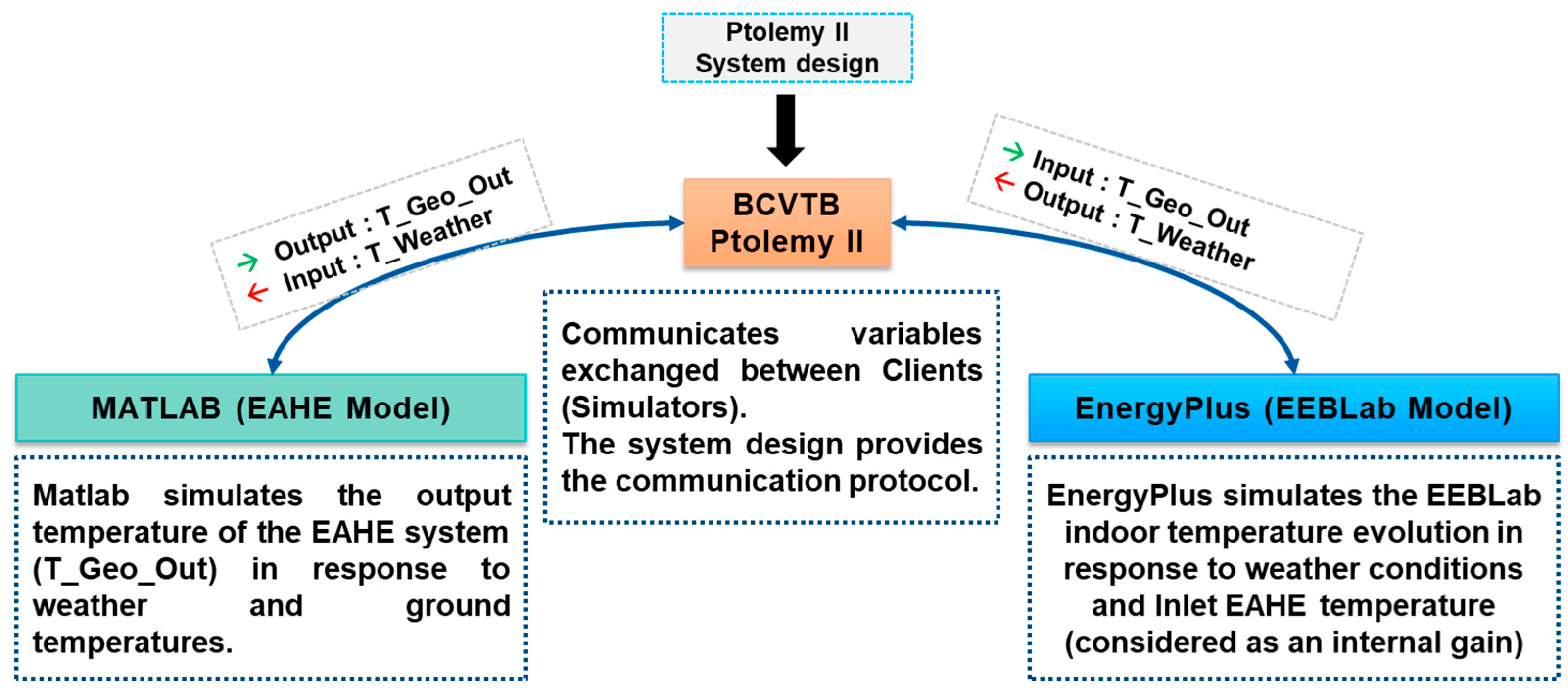
4. Co-Simulation Platform: Problem Formulation

In this work, the Buildings Controls Virtual Test Bed (BCVTB) was used as the main platform for co-simulation. The BCVTB framework links a diversity of simulation tools to serve our holistic approach. It is based on the Ptolemy II software environment and couples various simulation programs for distributed simulations. In our case, the main purpose is to simulate a small-scale building named EEBLab and an Earth-to-air heat exchanger in both the EnergyPlus and Matlab simulation tools. The main idea behind integrating the EAHE system into the EEBLab is to come up with an effective solution to cool and heat the building while reducing energy consumption. Hence, the BCVTB platform was used to evaluate the building performances with their different linked equipment and systems as a holistic complex system for more accurate simulations and results. The choice of BCVTB can be justified by many reasons. For instance, it has BACnet modules that directly read from and write to BACnet compatible controllers. Furthermore, BCVTB provides built linkages to connect simulation software tools, such as EnergyPlus, TRNSYS, Dymola and MATLAB. Ultimately, if we consider creating a hardware-in-the-loop platform, the co-simulation capability of the BCVTB makes it straightforward to realize time synchronization between the control hardware and simulation programs.

Figure 15 presents the communication flow between EnergyPlus and MATLAB through BCVTB. First, EnergyPlus communicates the weather data, extracted from the TMY/EPW weather file, to MATLAB which uses the external ambient air temperature as an input to run the simulation, resulting in a simulated outlet temperature of the EAHE system. It is then sent back as a geothermal heat gain to the EnergyPlus model to be considered among the heat balance algorithm and to compute the new zone temperature. Ptolemy II communicates the variables between the simulators since it is considered as an external interface. Once it is activated, all external interface objects will receive their value from the BCVTB framework or from the FMUs (functional mockup units) at each zone time step.

In our case, in order to take into account the EHAE system effect, an infiltration rate was defined (0.013 m³/s) to allow the zone inside air to be renewed three times per hour (as reported by ASHRAE standards). Furthermore, the energy management system (EMS) was also exploited. The first step was to define a fictive sensor inside the building to detect the zone internal temperature. The EMS-defined sensor reuses the normal output variables of EnergyPlus to provide a general way of obtaining a variety of input data with minimal complications. Once the sensor was defined and activated, the EMS program calling manager was activated to call a defined program developed by the user. Finally, EMS output variables were defined to obtain the required output data of the simulation. The EMS program was set to calculate indoor temperature, using mainly the same formula of the analytical solution.

The main purpose behind investigating the BCVTB platform is to allow the evaluation of energy systems linked to the considered building. This takes into account the real dynamics of the building in response to weather conditions as well as other indoor stimuli (occupants, internal loads, infiltrations, lighting, etc.).

A system evaluated in a standalone manner may not show its real performances and drawbacks. However, co-simulating the exchange of data occurs in real time and mimics the real responses of the system as if it was installed in a real case.

5. Results and Discussion

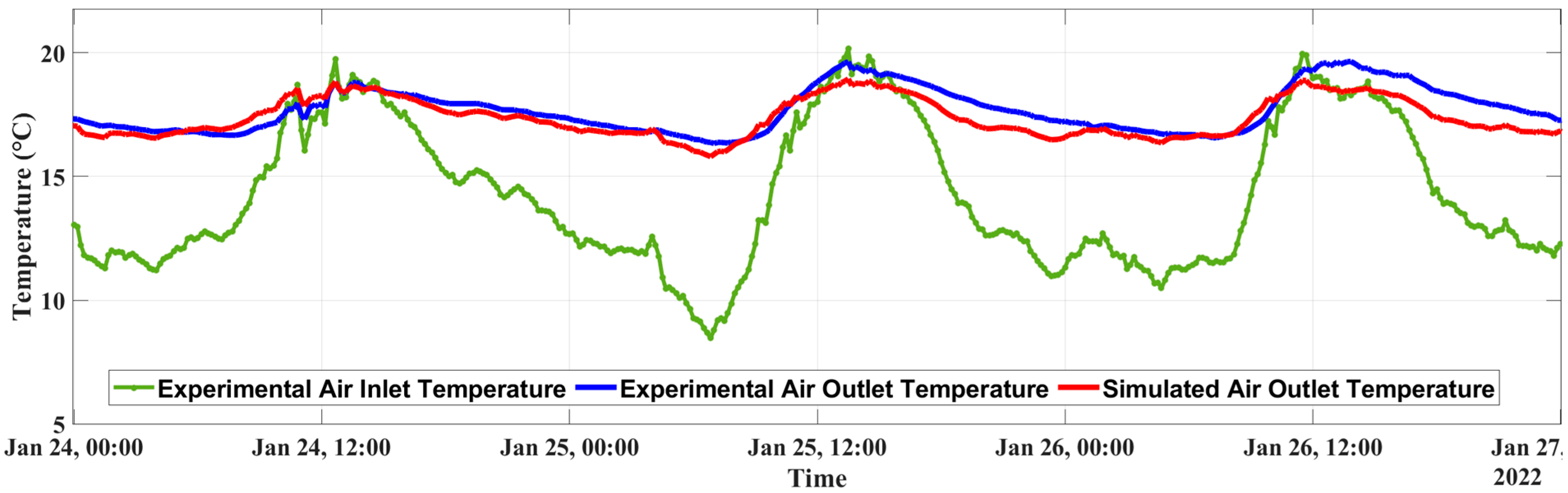
5.1. Earth-to-Air Heat Exchanger Standalone Simulation and Experimental Results

In what follows, we present the simulation and experimental results of the deployed EAHE system.

Figure 16 presents the simulation and experimental results for the period from 7 December 2021 to 2 February 2022. The preliminary observation shows that the EAHE system significantly decreases the fluctuation of the outdoor inlet temperature and maintains it at a more comfortable range from 15 to 20 °C.

Figure 17 is an example of two days of experimental and simulation results from 24 to 26 January 2022. As shown, the EAHE system brought the inlet air temperature from 8 °C to approximately 16 °C on 25 January at 06:50 and acted as a heater. The data collected from the experimental setup in this period as well as the simulation results revealed a significant correlation with a slight maximum deviation of 2 °C. Moreover, in Figure 18, the EAHE system acts as a cooler and decrease the inlet air temperature on 29 January at 13:50 from 23.45 to 20 °C in the outlet. The ground temperature for all the monitoring periods was about 19 °C.

The mean and maximum deviations for this model compared to the experimental setup were calculated, the mean deviation was about 3.82%, and the maximum reached 12.70%. Furthermore, the results of the Pearson correlation indicated that there was a significantly large positive relationship between the experimental and simulation outlet temperatures, (r(5559) = 0.849, p < 0.001).

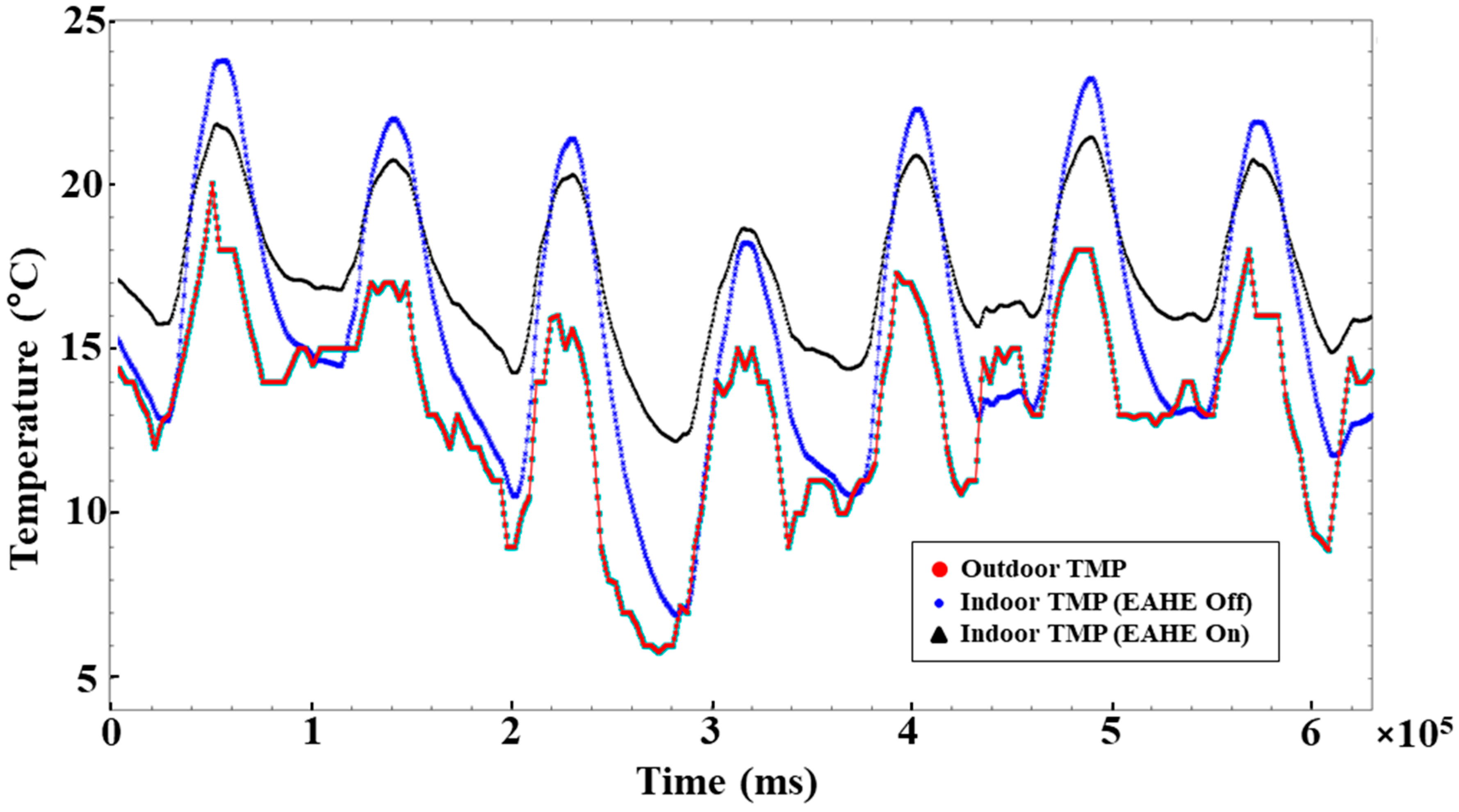
5.2. EAHE and EEBLab Experimental and Co-Simulation Results

In order to track the indoor temperature evolution of the EEBLab building, in response to external weather condition variations, a simulation using the EnergyPlus tool was performed for a period of 37 days. The simulation was run from 27 December 2021 to 2 February 2022, which is in line with the experimentation that is presented. An internal gain of 30 W was taken into account (wood table, equipment cabinet) in addition to 0.013 m³/s infiltrations.

Figure 19 presents the temperature evolution inside the EEBLab in response to external temperature variation. Both curves evolve, qualitatively, the same way. The temperature inside the zone reaches a maximum of 29.54 °C, while it reaches 31.32 °C outside. There is not much of a difference between both ambiances, which is mainly due to the fact that: (i) no heating or cooling devices are active; (ii) a window is placed on the south facade of the EEBLab; (iii) the envelope’s thermal inertia is weak since the walls are thick, although they are insulated.

In order to evaluate the accuracy of the obtained simulation results, we have conducted experiments by means of our deployed IoT and big data platform [31,32,33].

We used digital temperature sensors (DS18B20 and DHT22) connected to microcontrollers as sensing nodes. The sensors were connected to one wire (Parasite mode), and the I2C communication protocol was used to transfer data to the microcontrollers. The data was then transferred and visualized on our server. In our case, we created a custom weather station to monitor the outdoor environmental data (e.g., wind speed and direction, air pressure, ambient temperature and relative humidity, solar radiation) and placed it on the roof of the EEBLab, as previously shown in Figure 2. As for the indoor environmental data, we placed an embedded node with CO₂, ambient temperature and relative humidity sensors. Data sampling frequency was set to 10 s. This allows for an accurate temperature profile as well as for the application of different average periods for simulation or visualization.

Figure 20 presents the experimental temperature evolution inside the building in response to the external temperature variation. The internal and external temperatures almost had the same evolution tendency. The indoor temperature reached a maximum value of 31.10 °C, and the outdoor temperature reached a maximum of 31.32 °C.

Figure 21 is a presentation of the temperature deviation between the simulation and experimental results of the indoor temperature evolution. Concerning the indoor temperature, the difference between simulation and the experiment reached a maximum of 0.35 °C. This negligeable offset can be justified due to the sensor’s precision range as well as the input weather data average.

In this subsection, we present the results of the cooperative simulation by combining EnergyPlus and MATLAB to model the building and the EAHE system, using the BCVTB framework. The main objective is to be able to simulate the building as a complex system while taking into consideration its linked equipment. Furthermore, these results will allow for visualizing the influence of the EAHE system on the thermal comfort inside the EEBLab. In in order to study the correlation between the simulation and the experiments, real experimental outdoor temperatures were collected and used as input in the simulation. Using the collected outdoor environmental data of our test site, we updated an original EPW file and created a customized one with the collected temperatures using the Elements software. However, other ambient parameters (e.g., pressure, relative humidity, solar radiation) were not changed, since the variation was not influential.

The co-simulation was run for a period of 37 days from 27 December 2021 to 2 February 2022. Figure 22 presents the temperature evolution inside the building without the EAHE system activated (blue x-marked curve), with the EAHE activated (black triangle-marked curve) versus external temperature (red-dotted curve). For a better visualization of the results, the first 7 days are magnified (see Figure 23).

Without an EAHE device, the indoor temperature varied between a minimum of 5 °C and maximum of 25 °C. Once the EAHE was activated, the temperature evolved following the same pattern. However, it varied between a minimum of 12 °C and a maximum of 21 °C and remained at a comfortable temperature range. The EAHE reduced the indoor temperature of the EEBLab during the day by 2 °C and increased it during the night by 6 °C, which implies the crucial role that it plays in ensuring a comfortable range of temperature.

6. Conclusions

The main contributions of this paper are two-fold: The first is the evaluation of the performances of an Earth-to-Air heat exchanger in maintaining indoor thermal comfort in buildings. For this, a parametric study was run, and the most adequate parameter values were chosen to help us size the system and locally construct it. The second concerns shedding light on the importance of co-simulation approaches in evaluating system performances linked to buildings, in response to the actual real dynamic outdoor and indoor contexts. For this, the BCVTB framework was investigated to evaluate the EAHE performances while integrating it into the EEBLab. This platform allows for real-time data exchange between subsystems, namely, the EnergyPlus tool, which was used to simulate the indoor air temperature variations within the EEBLab and MATLAB to model the EAHE system and to calculate its performance based on various parameters. For validation purposes, a locally developed internet of things platform named HOLSYS was deployed to collect and monitor data from the sensors. The results proved to be a good agreement between both the experimentation and the simulation, in terms of the ability of the EAHE to maintain a comfortable indoor temperature range inside the EEBLab. Moreover, an economical modeling was created to evaluate the ability of such integrated systems in decreasing energy bills. It was shown that the power gained by using the EAHE system is about 1.4 kWh daily, resulting in 511 kWh per year, which mainly leads to a billing savings of MAD 827/year (USD 82).

Our future work will focus on the integration of the developed EAHE system with the heating ventilation and air conditioning (HVAC) system. The main aim will be to optimize the use of the HVAC system when the EAHE system is capable of satisfying the cooling and heating needs. Furthermore, using machine learning, we will be able to forecast the indoor environmental quality to control the systems according to the required comfort.

References

- Koenigsberger, J. The Temperature of the Earth’s Interior, Scientific American. Available online: https://www.scientificamerican.com/article/the-temperature-of-the-earths-inter/ (accessed on 4 April 2022).
- Kharbouch, A.; El Maakoul, A.; Bakhouya, M.; El Ouadghiri, D. Modeling and Performance Evaluation of an Air-Soil Exchange System in Energy Efficient Buildings. In Proceedings of the 2018 6th International Renewable and Sustainable Energy Conference (IRSEC), Rabat, Morocco, 5–8 December 2018; pp. 1–6. [Google Scholar] [CrossRef]
- Bhamare, D.K.; Rathod, M.K.; Banerjee, J. Numerical model for evaluating thermal performance of residential building roof integrated with inclined phase change material (PCM) layer. J. Build. Eng. 2019, 28, 101018. [Google Scholar] [CrossRef]
- Berrabah, S.; Moussa, M.O.; Bakhouya, M. Towards a thermo-mechanical characterization approach of buildings’ envelope. Energy Rep. 2020, 6, 240–245. [Google Scholar] [CrossRef]
- Pérez-Lombard, L.; Ortiz, J.; Pout, C. A review on buildings energy consumption information. Energy Build. 2008, 40, 394–398. [Google Scholar] [CrossRef]
- Sadineni, S.B.; Madala, S.; Boehm, R.F. Passive building energy savings: A review of building envelope components. Renew. Sustain. Energy Rev. 2011, 15, 3617–3631. [Google Scholar] [CrossRef]
- Peretti, C.; Zarrella, A.; De Carli, M.; Zecchin, R. The design and environmental evaluation of earth-to-air heat exchangers (EAHE). A literature review. Renew. Sustain. Energy Rev. 2013, 28, 107–116. [Google Scholar] [CrossRef]
- Sodha, M.; Bansal, N.; Seth, A. Variance of the ground temperature distribution. Appl. Energy 1981, 8, 245–254. [Google Scholar] [CrossRef]
- Bisoniya, T.S.; Kumar, A.; Baredar, P. Experimental and analytical studies of earth–air heat exchanger (EAHE) systems in India: A review. Renew. Sustain. Energy Rev. 2013, 19, 238–246. [Google Scholar] [CrossRef]
- Tiwari, G.N.; Singh, V.; Joshi, P.; Deo, A.; Gupta, A. Design of an Earth Air Heat Exchanger (EAHE) for Climatic Condition of Chennai, India. Open Environ. Sci. 2014, 8, 24–34. Available online: https://benthamopen.com/ABSTRACT/TOENVIRJ-8-24 (accessed on 19 January 2021). [CrossRef][Green Version]
- Antinucci, M.; Asiaín, D.; Fleury, B.; Lopez, J.; Maldonado, E.; Santamouris, M.; Tombazis, A.; Yannas, S. Passive and hybrid cooling of buildings–state of the art. Int. J. Sol. Energy 1992, 11, 251–271. [Google Scholar] [CrossRef]
- Touzani, N.; Jellal, J.E. Heating and cooling by geothermal energy: Canadian well-Case of Rabat. J. Mater. Environ. Sci. 2015, 6, 3268–3280. [Google Scholar]
- Moummi, N.; Benfatah, H.; Hatraf, N.; Moummi, A. Le rafraîchissement par la géothermie: Étude théorique et expérimentale dans le site de Biskra. J. Renew. Energ. 2010, 13, 399–406. [Google Scholar]
- Schloegl, F.; Rohjans, S.; Lehnhoff, S.; Velasquez, J.; Steinbrink, C.; Palensky, P. Towards a classification scheme for co-simulation approaches in energy systems. In Proceedings of the 2015 International Symposium on Smart Electric Distribution Systems and Technologies (EDST), Vienna, Austria, 8–11 September 2015; pp. 516–521. [Google Scholar] [CrossRef]
- Bleicher, F.; Duer, F.; Leobner, I.; Kovacic, I.; Heinzl, B.; Kastner, W. Co-simulation environment for optimizing energy efficiency in production systems. CIRP Ann. 2014, 63, 441–444. [Google Scholar] [CrossRef]
- Welsch, B.; Rühaak, W.; Schulte, D.O.; Formhals, J.; Bär, K.; Sass, I. Co-Simulation of Geothermal Applications and HVAC Systems. Energy Procedia 2017, 125, 345–352. [Google Scholar] [CrossRef]
- Cellura, M.; Guarino, F.; Longo, S.; Mistretta, M. Modeling the energy and environmental life cycle of buildings: A co-simulation approach. Renew. Sustain. Energy Rev. 2017, 80, 733–742. [Google Scholar] [CrossRef]
- Cucca, G.; Ianakiev, A. Assessment and optimisation of energy consumption in building communities using an innovative co-simulation tool. J. Build. Eng. 2020, 32, 101681. [Google Scholar] [CrossRef]
- Yao, J. Determining the energy performance of manually controlled solar shades: A stochastic model based co-simulation analysis. Appl. Energy 2014, 127, 64–80. [Google Scholar] [CrossRef]
- Corrado, V.; Fabrizio, E. Steady-State and Dynamic Codes, Critical Review, Advantages and Disadvantages, Accuracy, and Reliability. In Handbook of Energy Efficiency in Buildings; Butterworth-Heinemann: Oxford, UK, 2019; pp. 263–294. [Google Scholar] [CrossRef]
- Walton, G.N. Thermal Analysis Research Program Reference Manual; US Department of Commerce, National Bureau of Standards: Washington, DC, USA, 1983; p. 21. [Google Scholar]
- Yazdanian, M.; Klems, J. Measurement of the Exterior Convective Film Coefficient for Windows in Low-Rise Buildings. ASHRAE Trans. 1993, 100, 2. [Google Scholar]
- Bisoniya, T.S. Design of earth–air heat exchanger system. Geotherm. Energy 2015, 3, 1266. [Google Scholar] [CrossRef]
- Hollmuller, P.; Lachal, B. Air–soil heat exchangers for heating and cooling of buildings: Design guidelines, potentials and constraints, system integration and global energy balance. Appl. Energy 2014, 119, 476–487. [Google Scholar] [CrossRef]
- T’Joen, C.; Liu, L.; Paepe, M. Comparison of Earth-Air and Earth-Water Ground Tube Heat Exchangers for Residentialal Application. In Proceedings of the International Refrigeration and Air Conditioning Conference, Purdue, IN, USA, 16–19 July 2012; Available online: https://docs.lib.purdue.edu/iracc/1209 (accessed on 1 May 2022).
- Losses in Pipes. Available online: https://me.queensu.ca/People/Sellens/LossesinPipes.html (accessed on 2 June 2022).
- Head Loss-Pressure Loss|Definition & Calculation|nuclear-power.com. Nuclear Power. Available online: https://www.nuclear-power.com/nuclear-engineering/fluid-dynamics/bernoullis-equation-bernoullis-principle/head-loss/ (accessed on 6 July 2022).
- Addendum n to ANSI/ASHRAE Standard 62-2001; Ventilation for Acceptable Indoor Air Quality. ASHRAE: Atlanta, GA, USA, 2001; p. 13.
- Lai, C.S.; Jia, Y.; Xu, Z.; Lai, L.L.; Li, X.; Cao, J.; McCulloch, M.D. Levelized cost of electricity for photovoltaic/biogas power plant hybrid system with electrical energy storage degradation costs. Energy Convers. Manag. 2017, 153, 34–47. [Google Scholar] [CrossRef]
- Lai, C.S.; Locatelli, G.; Pimm, A.; Tao, Y.; Li, X.; Lai, L.L. A financial model for lithium-ion storage in a photovoltaic and biogas energy system. Appl. Energy 2019, 251, 113179. [Google Scholar] [CrossRef]
- Malek, Y.N.; Kharbouch, A.; El Khoukhi, H.; Bakhouya, M.; De Florio, V.; El Ouadghiri, D.; Latre, S.; Blondia, C. On the use of IoT and Big Data Technologies for Real-time Monitoring and Data Processing. Procedia Comput. Sci. 2017, 113, 429–434. [Google Scholar] [CrossRef]
- Kharbouch, A.; El Khoukhi, H.; Nait Malek, Y.; Bakhouya, M.; De Florio, V.; El Ouadghiri, D.; Latré, S.; Blondia, C. Towards an IoT and Big Data Analytics Platform for the Definition of Diabetes Telecare Services. In Proceedings of the Smart Application and Data Analysis for Smart Cities, Casablanca, Morocco, 28 May 2018. [Google Scholar] [CrossRef]
- Kharbouch, A.; Bakhouya, M.; El Maakoul, A.; El Ouadghiri, D. A Holistic Approach for Heating and Ventilation Control in EEBs. In Proceedings of the 17th International Conference on Advances in Mobile Computing & Multimedia, Munich, Germany, 2–4 December 2019. [Google Scholar] [CrossRef]