Energy-Based Prognostics for Gradual Loss of Conveyor Belt Tension in Discrete Manufacturing Systems

Abstract

This paper presents a data-driven approach for the prognosis of the gradual behavioural deterioration of conveyor belts used for the transportation of pallets between processing workstations of discrete manufacturing systems. The approach relies on the knowledge of the power consumption of a conveyor belt motor driver. Data are collected for two separate cases: the static case and dynamic case. In the static case, power consumption data are collected under different loads and belt tension. These data are used by a prognostic model (artificial neural network (ANN)) to learn the conveyor belt motor driver’s power consumption pattern under different belt tensions and load conditions. The data collected during the dynamic case are used to investigate how the belt tension affects the movement of pallets between conveyor zones. During the run time, the trained prognostic model takes real-time power consumption measurements and load information from a testbench (a discrete multirobot mobile assembling line) and predicts a belt tension class. A consecutive mismatch between the predicted belt tension class and optimal belt tension class is an indication of failure, i.e., a gradual loss of belt tension. Hence, maintenance steps must be taken to avoid further catastrophic situations such as belt slippages on head pulleys, material slippages and belt wear and tear.

1. Introduction

Modern discrete manufacturing systems are composed of different industrial machines and equipment, which are prone to different faults. The consequences of these faults range from a soft inconvenience to life-threating situations. Furthermore, for production systems, there is a certain cost associated with every occurrence of a fault, which includes a production line shutdown, the possible repair or collateral damage of parts and labour for replacing the failed component or machinery [1]. In addition to this, the gradual deterioration of devices or equipment of a production system significantly contributes to the downtime of production machines or other heavy-duty equipment [2]. Gradual equipment deterioration remains unnoticed until the effects become enormous enough to disrupt normal working operations. The maintenance cost associated with equipment faults has a significant impact on an organization’s revenue. According to study [3], the gradual wear of equipment is responsible for a 3% to 8% decrease in oil production, causing up to USD 20 billion losses in the US economy.

As a result of the associated risks and costs of failures, early-stage equipment failure detection and prognostic maintenance is crucial to avert serious disruptions to production systems. To detect incipient equipment wear, data from plant sensors are utilized, for example, data from vibration, temperature, pressure and humidity sensors used in online maintenance [4]. In addition to the above-mentioned sensor data, energy consumption patterns associated with equipment or pieces of equipment are also a promising criterion for determining gradual equipment failure [5,6], an example of such a fault is the gradual loss of belt tension in conveyor-belt-operated transportation systems in discrete manufacturing systems.

The main objective of this research is building an AI-based system that allows for the monitoring of production equipment wear and tear. More precisely, in this work, the power consumption of the conveyor belt motor driver is repeatedly observed for a range of belt tensions and workloads. The obtained information is used along with real-time power consumption and workload information coming from the testbench to detect a gradual loss of belt tension. This tension can then be used for estimating the working life span of the belts. The envisioned advantage of such a system is the ability to continually monitor the state of the production, which, in return, permits a rapid and efficient maintenance with minimum equipment downtime.

This paper is organized as follows: Section 2 briefly presents the theoretical background of this work and related research. Section 3 describes the testbed used. Section 4 provides the details on the method used for detecting the gradual loss of belt tension in a conveyor belt within a defined factory automation setting. Section 5 presents the data analysis and results. Section 6 concludes and outlines future work.

2. Background

2.1. Maintenance Strategies

The performance of a production system is significantly influenced by the maintenance strategies adopted by the site managers. On the one hand, a good and effective maintenance policy increases the equipment/machine life, thereby ensuring it is readily available for use. On the other hand, an ineffective or poor maintenance strategy decreases the equipment life as well as its time of availability, and this leads to unexpected and sudden breakdowns. There are two types of maintenance policies used in the industry, namely, reactive and proactive maintenance. The reactive maintenance policy includes the Run-2-Failure strategy and proactive maintenance includes both preventive and predictive maintenance strategies [7].

Run-2-Failure and preventive maintenance are the two major maintenance strategies used for production systems. The Run-2-Failure maintenance strategy (also known as the reactive, fault-driven or fire-fighting maintenance strategy) is a maintenance strategy where maintenance activity starts when either an obvious equipment functional failure, malfunction or equipment breakdown occurs. As it is a reactive maintenance strategy, the corrective measurements are governed by random failure events and sometimes these failures lead to very large equipment or machine downtimes, an extensive equipment repair time as well as high repair cost, which decrease production in the manufacturing system [7,8,9,10].

Preventive maintenance, also known as time-based maintenance, helps to slow down the equipment deterioration through planned periodic plant inspections and repairs, for example, periodic lubrication and calibration, etc. [8]. In the preventive maintenance strategy, the part for maintenance is replaced on a specific date and this ensures that there is a low possibility of sudden failure. In comparison to Run-2-Failure, preventive maintenance provides more safety, since a part failure is not likely prior to maintenance. However, the preventive maintenance strategy is not cost-efficient, because some parts would be functional after removal, thus, making the replacement unnecessary [11,12].

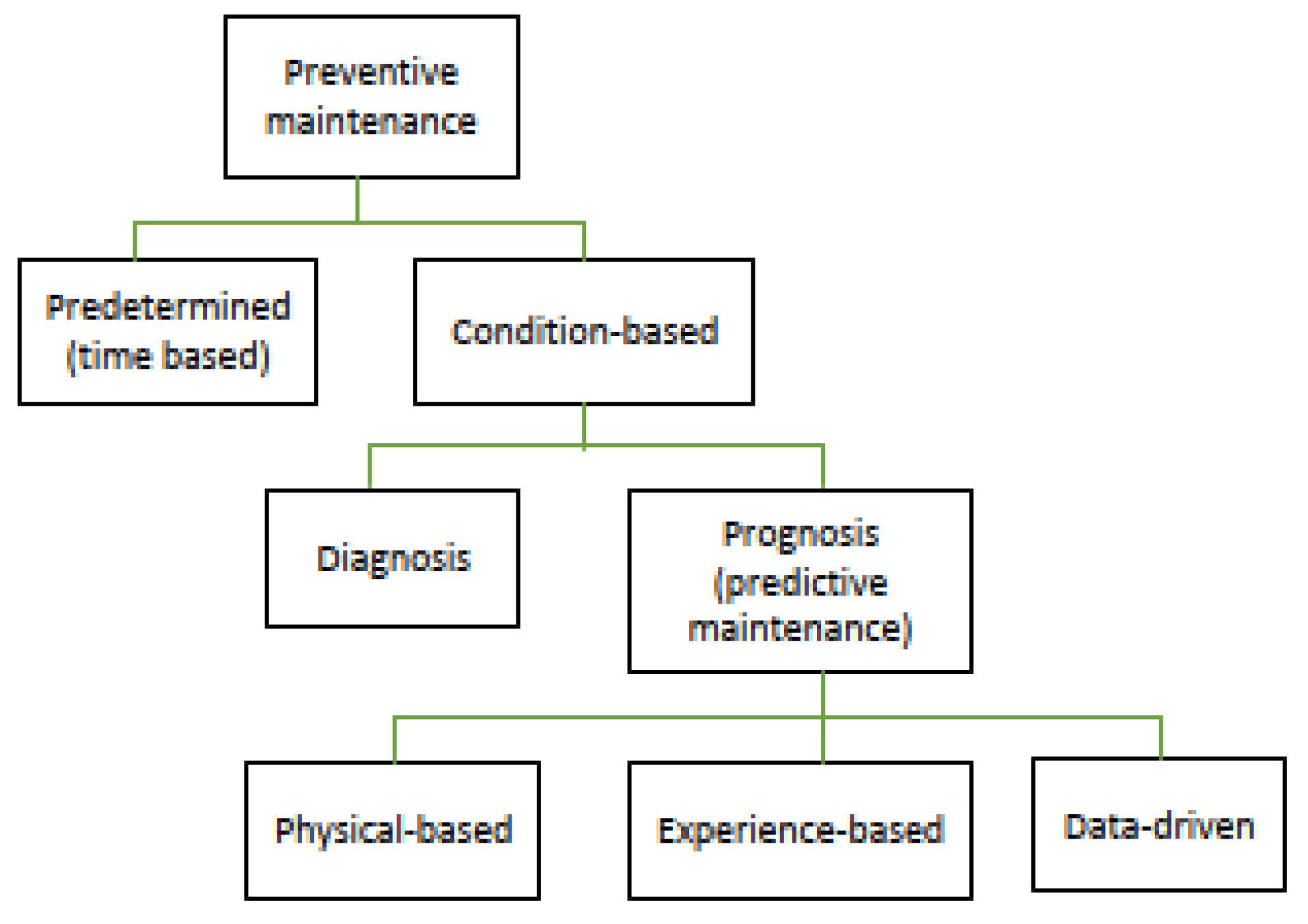
Predictive maintenance, which is a type of condition-based maintenance, uses prognostic models to foretell the equipment, component, or machine condition. These prognostic models continuously monitor the under-test equipment’s or component’s parameters using sensors such as energy analyser modules, temperature, vibration, corrosion, humidity, etc., for the purpose of building a training model so that the model can foretell/predict the failure in the equipment before it occurs [8,11,12,13]. Figure 1 shows the taxonomy of predictive maintenance.

At the state-of-the-art, fault detection methods are either data-driven or model-driven. Model-driven fault prognosis uses a mathematical model of a system as a reference for analysing the new incoming data from equipment. However, these models do not need any historical data for learning the system’s parameters. The main challenge of this approach is ensuring the accuracy of the developed model as the system complexity increases with technological enhancements [14].

Data-driven models are based on historical observations of data coming from a process or equipment. For a data-driven fault prognosis system, a mathematical model is not required [15,16]. Data-driven models learn the system’s behaviour through machine learning (ML) techniques and statistical algorithms, for example, an artificial neural network (ANN) or support vector machine (SVM). Data-driven models are applied for foretelling faults when the basic operating principle of a system is hard to model, or if a system is very complex. Data-driven models are data-dependent, and this poses a big challenge as they require huge amounts of good-quality data for training [17]. Depending on the application, data-driven models may require good-quality data of up to two years.

State-of-the-art predictive maintenance techniques are either passive or active [18]. Passive maintenance techniques either use output signals from already existing on-site sensors and verify performance themselves or use on-site installed test sensors to monitor the desired parameters (pressure, energy analysers, vibration, etc.). The installed sensor’s output signals are then used to judge the performance by comparing the results with the expected results [4]. On the other hand, active maintenance techniques allow users to inject test signals into the equipment in real-time to observe the equipment’s response to the injected input as well as its modifications.

For predictive maintenance, data-driven prognostic models are mostly used to predict equipment anomalies or the gradual deterioration of a component. Therefore, for a good quantification of machine/equipment faults, data-driven models need a huge amount of good-quality data for training a machine learning (ML) or deep learning (DL) regression or classifier model. For example, in [19], real-time vibration data were collected until the point of failure to create a vibration-based database of suitable amplitudes associated with the bearing defective frequency and its first five harmonics.

2.2. Artificial Neural Network

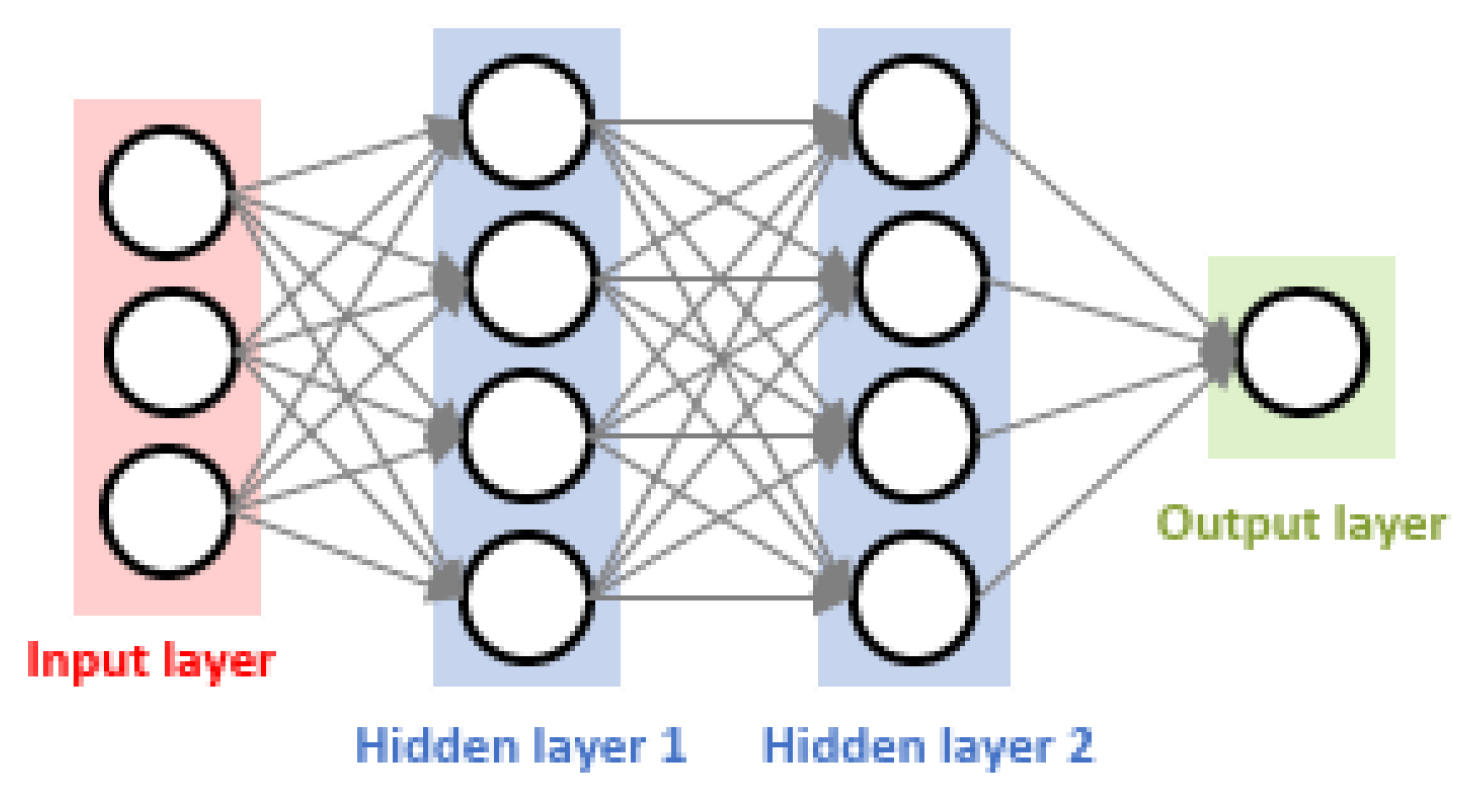
Machine learning (ML) and deep learning (DL) algorithms can be used for predicting anomalies in industrial equipment or in a machine part. ML algorithms learn the system’s behaviour and patterns from training data. The trained model is then used to determine prediction on new incoming sample data. Deep learning (DL) is a subset of ML algorithms that uses one or more hidden layers with several processing neurons known as nodes (Figure 2) [20]. Figure 2 shows a simple artificial neural network (ANN) with one input layer accompanied by three nodes representing the data coming from sensors or desired equipment parameters, two hidden layers with four processing nodes and one output layer with one node. ANNs are good at function approximation and system parameter learning with feed-forward and back-propagation, respectively. This learning process is extensively discussed in [21,22,23].

Different deep learning variants, such as artificial neural networks (ANNs), convolutional neural networks (CNNs), long short-term memory (LSTM) and recurrent neural networks (RNNs), are widely used in predictive maintenance due to their inherent ability to capture, learn and retain nonlinear failure patterns [24]. In [21,25], the authors extensively reviewed the DL algorithms, architectures and methodologies (supervised, unsupervised or hybrid) used for predictive maintenance and presented a case study of engine failure predictions. According to [26], ANNs differ from traditional statistical techniques in their ability to successfully learn nonlinear features of a time series. ANNs have been widely used in forecasting equipment health and failures. DL is also making its way into predictive maintenance day by day. Besides their positive aspects, deep learning models have a negative aspect. DL models require very large amounts of data in order to perform better than other techniques. They are extremely expensive to train due to the complex data models.

3. Testbench

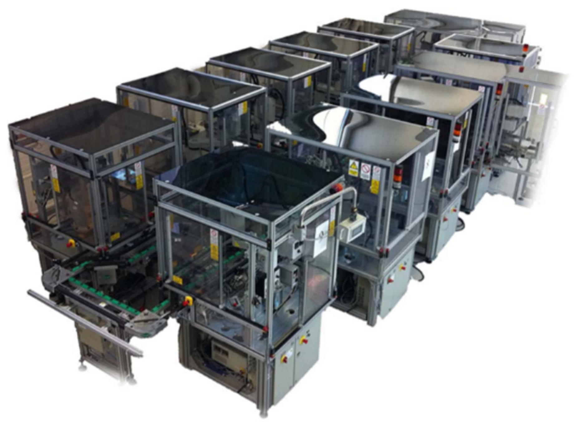
The FASTory production assembly line (Figure 3) [27] was used as a testbench in this research work. In the past, the FASTory line was used in a factory to assemble cell phone parts such as frames, keypads and screens. After retrofitting the FASTory line, it now simulated its original cell phone assembling operations by drawing main cell phone parts (frames, keypads and screens) in different shapes and colours onto paper carried by a pallet. 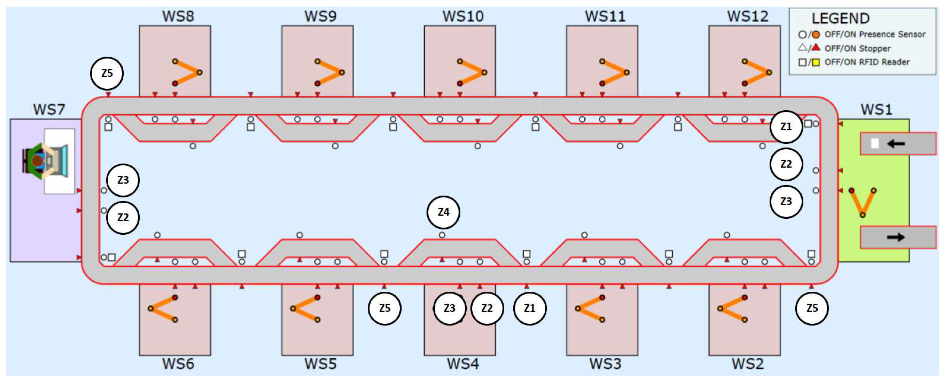Figure 4 [27] shows the layout of the FASTory line.

The FASTory production assembly line comprised ten identical workstations, one buffer station and one paper loading and unloading station. WS7 was the pallet buffer station, which was used for loading and unloading empty pallets, and WS1 loaded paper onto pallets for drawing and then unloading the paper containing the complete drawing of a selected cell phone model. The remaining ten processing workstations were labelled WS2–WS6 and WS8–WS12. Each of these workstations had one main and bypass conveyor. Of these workstations, workstations 3, 4, 5 and 8 had six six-axis robots from KUKA, ABB and Omron, while workstations 2, 6 and 9–12 had one SONY SCARA robot. WS1 had a dual-arm YASKAWA robot.

On each production workstation, the main conveyor transferred a pallet to the robot, and a bypass conveyor transferred the pallet to the next available station when the workstation was busy. The FASTory line followed the closed loop topology which provided an uninterrupted path for pallets, thereby increasing the productivity/space ratio. The two conveyors split into different zones, which are marked in Figure 4 and referred to as Z# in this paper. The entry and exit points of the workstations were located at Z1 and Z5, respectively. The main conveyor had four zones (Z1, Z2, Z3 and Z5), and for each zone there was a stopper and presence sensor for stopping a pallet and checking the presence of a pallet. Z3 was the production zone of each workstation. The Z1 of each workstation had a RFID tag reader, which was used to read the pallet ID. The Z1 of the current workstation and Z5 of the next workstation were the same. The bypass conveyor had one zone (Z4) and one stopper.

The FASTory line was equipped with anS1000 logical controller and an E10 energy analyser module. The S1000 is a smart, web-service-enabled controller, which is used for invoking operations and managing shop floor equipment and devices. Besides providing the functionalities of a genetic controller, the S1000 is capable of exposing equipment data and methods from the production line as RESTful services [28]. Among such services is the event subscription mechanism, which enables event-driven behaviour in the system. The exposed event notifications (

Table 1. Event notification from testbench.

S/N	Event Notification	Description
1	EnergyMeter	Robot/conveyor/controller energy consumption of each working cell published at a time interval of one second
2	DrawStart/DrawEnd	Cell ID, recipe number, pen colour and time stamp
3	EquipmentState	Cell ID, state of conveyor zones, pallet ID and time stamp

) include information about energy consumption (via the S1000 energy meters) and CAMX state events (e.g., pallet input to a conveyor piece, etc.).

4. Prognosis of Gradual Loss of Belt Tension in Conveyor-Belt-Operated Transportation System

Conveyor belts are used to transport different materials over long distances in different industrial environments, such as mining, metallurgy, etc. In discrete production systems, conveyor belts are used to transport equipment, pallets and other tools between workstations. Belt conveyors are ideal for the efficient transfer of goods and materials over long distances. To achieve efficient material transport, conveyor belts need a certain traction force and belt tension to overcome the path friction. The traction force is provided by the conveyor motor driver engine. The belt motor driver power and belt tension are calculated by following the procedures defined in DIN and CEMA standards [29,30]. Once the parameters such as the horsepower (hp) required at the drive of a belt conveyor, effective belt tension, ambient temperature factor, idler friction factor, etc., are calculated, the belt conveyor system is installed and the nominal belt tension is adjusted for efficient material transportation.

The loss in belt tension is a gradual process and remains undetected until some serious faults occur in the transportation system, or significant belt wear is observed. Excessive and insufficient belt tensions are harmful for conveyor belts. Insufficient belt tension leads to belt slippage at the head pulley, excessive heat generation, belt wear and tear (damaged rubber belts) and unexpectable delays in material transportation. Conversely, excessive belt tension leads to excessive stress on the motor shaft, bearings and belts, and this can damage the driver motor. It could also lead to belt mistracing issues and uneven belt wears.

Traditionally, operators perform weekly, bi-weekly or monthly inspections of conveyor belts to keep the system healthy and in good working condition, i.e., by following a scheduled preventive maintenance strategy; however, to carry this out, they need to stop the whole production plant or a section of the production plant, and this decreases the plant production efficiency. This preventive maintenance strategy can be replaced with a predictive maintenance strategy by carefully selecting and monitoring the parameters which describe the behaviour of the conveyor belt and are able to show parameter variations as soon as the belt tension starts deviating from the nominal value. These parameters could be the data coming from vibration sensors, driver motor temperature, power consumed by driver motor, etc.

In this paper, the power consumed by the motor driver and the load on the conveyor belt were the parameters of interest used for investigating the relationships between the driver motor power consumption, belt tension and load and for predicting the belt tension. Insufficient belt tension was determined with the developed prognostic model based on the real-time power consumption of the motor driver of the conveyor and the load on the conveyor belt. The prognostic model learned the conveyor belt’s power consumption patterns under different belt tensions and load configurations and then predicted a belt tension class. A consecutive mismatch between the predicted belt tension class and optimal belt tension class was an indication of failure, i.e., a gradual loss of belt tension.

4.1. Monitoring Relevant Testbench-Generated Data

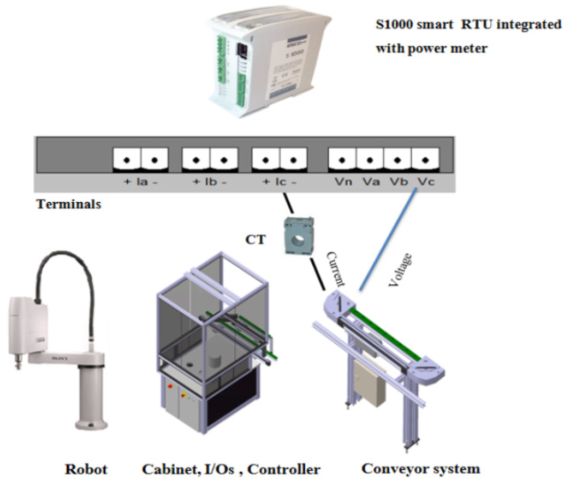
In this paper, the relevant data generated from the testbench were related to the power consumed by the conveyor belt motor driver. As mentioned in Section 3, all the workstations of the FASTory line were equipped with an E10 energy analyser module, which is an expansion module to the S1000 controllers and provides three-phase electrical power consumption monitoring (See Figure 5) [2]. Phase A was assigned to the robot, Phase B was allocated to the cabinet, I/Os and the controller, while Phase C was assigned to the conveyor system (including main and bypass conveyors). Power was measured with sampling current and voltage. The current sampled with a current transformer (CT) (which measured the high voltage current) was connected to the +Ia−, +Ib− and +Ic− terminals. The voltage was measured through a direct connection of the three phases (Va, Vb and Vc) and the neutral (Vn) terminals of the E10 expansion module. The Phase C energy values were of interest in this paper.

4.2. Data Collection, Preparation and Feature Extraction

In the course of this work, data were collected separately for the “static case and dynamic case”. In the static case, stoppers at the zones of the main conveyor were active all the time, and the main conveyor was kept running continuously irrespective of whether the pallets residing on the conveyor were stopped via stoppers or not. When the stoppers were in use, there was an increase in friction between the conveyor belt and the pallet, which resulted in an increase in power consumption in the conveyor belt motor driver. While collecting data for the static case, the load on the conveyor and the belt tension was varied according to

Table 2. Pallet position on main conveyor’s zones with respect to load combinations.

Load Combination	Active Zones	Description
0	0000	No load
1	1000	1 pallet at Z1
2	0100	1 pallet at Z2
3	1100	2 pallets; 1 pallet at each zone (Z1, Z2)
4	0010	1 pallet at Z3
5	1010	2 pallets; 1 pallet at each zone (Z1, Z3)
6	0110	2 pallets; 1 pallet at each zone (Z1, Z3)
7	1110	3 pallets; 1 pallet at each zone (Z1, Z2, Z3)
8	0001	1 pallet at Z5
9	1001	2 pallets; 1 pallet at each zone (Z1, Z5)
10	0101	2 pallets; 1 pallet at each zone (Z1, Z5)
11	1101	3 pallets; 1 pallet at each zone (Z1, Z2, Z5)
12	0011	2 pallets; 1 pallet at each zone (Z3, Z5)
13	1011	3 pallets; 1 pallet at each zone (Z1, Z3, Z5)
14	0111	3 pallets; 1 pallet at each zone (Z2, Z3, Z5)
15	1111	4 pallets; 1 pallet at each zone (Z1, Z2, Z3, Z5)

and

Table 3. Head pulley position and % belt tension.

Head Pulley Position (cm) from Initial Point	% Belt Tension
0	0
0.4	15
0.81	30
1.22	45
1.62	60
1.89	70
2.02	75
2.29	85
2.43	90
2.57	95
2.7	100

, respectively. As mentioned in Section 3, the main conveyor had four zones (Z1, Z2, Z3 and Z5), which were the active zones, so there were 16 possible combinations to place a pallet (load) on a conveyor. In Table 2, the active zone column lists all the possible combinations for the active zones. Here, “1” means the presence of a pallet on a zone and “0” the absence of a pallet on a zone. Each of these combinations was assigned a decimal number from 0 to 15, which was listed in the first column (load combinations).

The data collected in the static case helped to investigate the lower threshold (minimum belt tension that induced motion in the belt under a “no-load” condition) and the upper threshold values of the belt tension. Furthermore, they provided information about how the active zone on the conveyor belt affected belt slippage and power consumption of the belt motor driver for different belt tensions. In addition, the data from the static case were used for training the ANN model. On the other hand, for the dynamic case, only the conveyor belt was kept running all the time, and stoppers were not active all the time but controlled by web services provided by the FASTory line. The topic of interest was to investigate how the belt tension affected the movement of pallets between conveyor zones, as well as the transportation of material/tool/equipment between workstations. The movement of a pallet between zones was further divided into two cases; in case one, a pallet could move from the source to the destination zone on the main conveyor, and no pallet resided on the remaining zones. In case two, one or more pallets resided on the zone when a pallet moved from the source to the destination, and these zones were listed in the “active zone” column.

The power consumed by the motor driver had a direct relationship with the tension in the conveyor belt and the load on the conveyor, i.e., the number of pallets occupying the conveyor at a time. As mentioned in Section 3, the conveyor paths of the FASTory line were divided into zones, and for the same belt tension, the presence of a pallet in different zones had different effects on the power consumption of the driver motor. The power consumption data were collected for all zones according to the zone combinations shown in Table 2. The belt tension of the main conveyor could be varied by moving the head pulley upward or downward, as shown in Figure 6. The green arrow points towards a decrease in belt tension, while the red arrow points towards an increase in belt tension. The belt tension was varied from 0% to 100% by adjusting the head pulley position between a 0 and 2.7 cm adjustable distance. This became necessary as it was important to determine the optimal belt tension range of the head pulley. The belt tension was increased gradually to determine the lowest belt tension required to set the conveyor belt in motion. The belt tension was first increased from 0% to 60% at 15% intervals until the belt started touching the head pulley of the motor driver. Following this, the belt tension was increased by 10%. At 70% belt tension, the conveyor belt started moving without any load, but as soon as a pallet was placed on the conveyor, a jerky motion was observed. The belt tension was then increased by 5% to check how it affected the power consumption, the pallet transportation and how it differed from the previously collected data. Following this, the belt tension was increased at 10% intervals until reaching 95% belt tension. The head pulley was then moved all the way down to the maximum belt tension of 100%, thereby corresponding to 11 different positions of the head pulley. The data collection process lasted for one week. Table 3 lists the head pulley positions and corresponding percentages of belt tension.

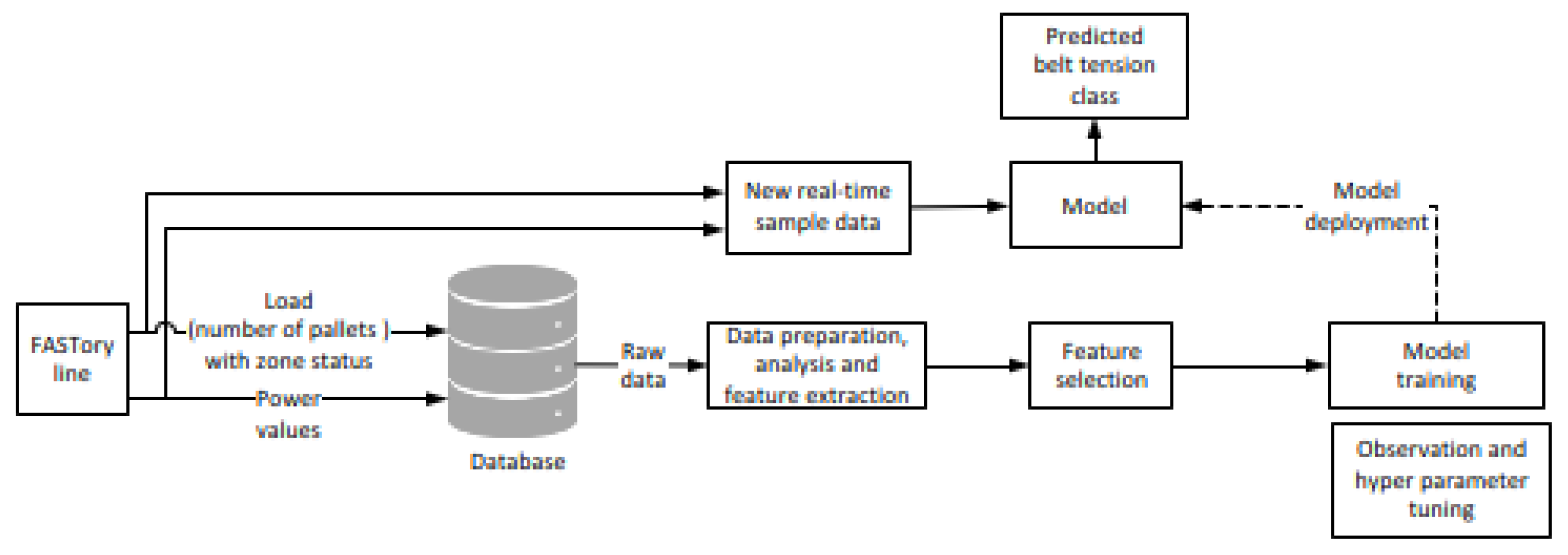
In Figure 7, the main steps for the development of the data-driven prognostic model for predicting the belt tension class is illustrated. The data were collected from the FASTory line during the static case and stored in a database for processing, analysis and feature extraction at a later stage. During the collection of data, the load on the conveyor belt and belt tension was varied according to Table 2 and Table 3 to monitor the effect of the active zone (i.e., the zone on which the pallet resided) and investigate the lower threshold value (smallest belt tension required to set the belt in motion) for belt tension, respectively. After storing the raw data in the database, the next step was to retrieve, process and prepare the data for analysis and feature extraction. Following that, the features were modified according to the ANN model requirements. Afterwards, the data were exposed to the ANN model for training and hyperparameter tunning. During this phase, activation functions for layers, the number of hidden layers and nodes in layers were changed until a good value was obtained for both loss and accuracy. This was important for the training and validation phases. The final version of the ANN model contained one input layer and two inputs (power and load values), and a “relu” activation function was used. There was one output layer with a “softmax” activation function and there were two hidden layers with a “relu” activation, with each hidden layer having 10 nodes. This model used “L2 regularisation” to avoid overfitting, and for optimization, the “adam” optimizer was used. The ANN model was trained on 80% of data, 10% of data was used for validation and the remaining 10% was used for model testing. After finishing all the steps, the model was deployed for consuming real-time data coming from the FASTory line and predicting the belt tension class.

5. Data Analysis and Results

In this section, the data collected for both static and dynamic cases were analysed thoroughly for each belt tension against all load combinations. As mentioned earlier in Section 4, both “too high” and “too low” belt tensions are harmful to a conveyor belt. Therefore, an analysis of the static case data helped to investigate the lower threshold and upper threshold values of belt tension. Furthermore, it also provided information about how active conveyor belt zones affected the belt slippage and power consumption of the belt motor driver. The analysis of data collected under the dynamic case was used to investigate how the belt tension affected the pallet movement between the conveyor zones and workstations of the FASTory line.

5.1. Results and Analysis for 0% to 70% Belt Tension

During the static phase of the experiment, the belt tension was gradually increased from 0% to 95% according to Table 3, and the load was varied on the conveyor belt according to Table 2. For belt tension between 0% and 60%, it was concluded that the belt tension values were not useful for any operation, because for these belt tensions, a sufficient frictional driving force was not generated between the head pulley (driving wheel) and the conveyor belt, which led to belt slippage. After a 10% increase in belt tension (i.e., 70% belt tension), the conveyor motor driver was able to provide enough traction force to overcome path resistances and set the conveyor belt into motion without any load on the conveyor belt and at a very low speed. For 70% belt tension, only load combinations 0 and 1 were used to collect the power consumption data, because in the static case, stoppers on each zone were active, and this increased the resistance between the conveyor belt and the conveyance path.

Therefore, as soon as there was a pallet on Z1 (zone one), the belt speed significantly reduced, the belt started slipping from the head pulley and a jerky motion was observed. This was because the provided traction force from the motor driver was not enough to overcome the conveyance path resistance. This jerky motion is harmful to conveyor belt health and can cause belt wear and tear, which reduces belt life. Figure 8 shows the box plots for the belt tension ranging from 0% to 70%, where the circles on boxes represent the data mean. It can be seen from the boxplots that as soon as the conveyor belt started moving at 70% belt tension with no load, the power consumption of the motor driver increased due to the generation of tractional driving force between the belt and head pulley. In contrast, a decrease in the motor driver power consumption was observed as soon as there was a pallet on Z1 of the conveyor. The reason was because the traction force generated with this belt tension was not enough to overcome the conveyance path friction, leading to a jerky movement due to the slipping of the conveyor belt from the head pulley.

Table 4. Dynamic case results for 70% belt tension.

Belt Tension (%)	Act. Zone	Src. Zone	Dst. Zone	Distance (m)	Time (s)	Speed (m/s)
70	No	1	5	1.61	120	0.013
70	No	1	2	0.61	80	0.008
70	No	1	3	0.835	86	0.01
70	No	3	5	0.773	inf	0

presents the results for the dynamic case data, which show how 70% belt tension affected the pallet movement between different zones of the conveyor belt, while also indicating the status of the active zone (Act. Zone). The pallet was moved between the source zone (Src. Zone) and the destination zone (Dst. Zone) of the conveyor. The distance between zones on the conveyor was fixed (i.e., Z1 to Z5 at 1.61 m, Z1 to Z2 at 0.61 m, Z1 to Z3 at 0.835 m and Z3 to Z5 at 0.773 m) and the time taken by a pallet was noted to obtain the speed of the conveyor belt. For this belt tension, it took 120 s for a pallet to move from Z1 to Z5. In addition, belt mistracking was observed when the pallet moved between Z3 and Z5, as the pallet was stuck at the junction where the bypass conveyor met the main conveyor, thereby preventing the pallet from reaching Z5 and, as such, the transportation time was infinite (inf), as presented in Table 4.

From the analysis of results obtained from the static and dynamic cases, it was concluded that 70% belt tension was the lower threshold value, i.e., minimum belt tension, which set the belt into motion without any load on the conveyor belt. However, this belt tension was not suitable for material transportation, because the generated traction force was not enough to overcome the conveyance path friction as the belts started slipping from the head pulley.

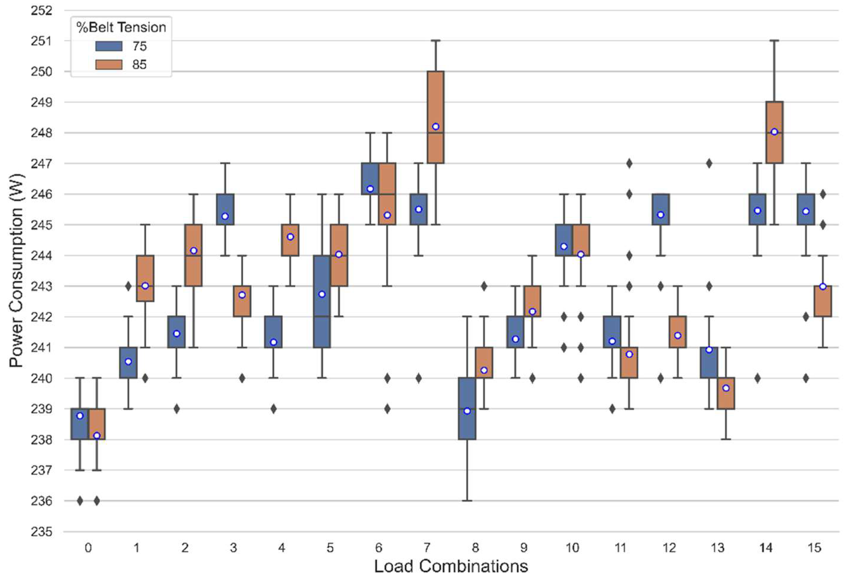
5.2. Results and Analysis for 75% to 85% Belt Tension

The results obtained for 75% belt tension with the load combinations 6, 7 and 14 (i.e., Z2 and Z3 were active for each combination) and 15 (all zones were active) were prominent. For these combinations, a reduction in the belt traction force and an increase in belt slippage was observed. For 85% belt tension, either no reduction in the belt traction force or an increase in belt slippage was observed. For these belt tensions, the experiment was conducted for all load configurations, i.e., the experiment was repeated for every load combination listed in Table 2. 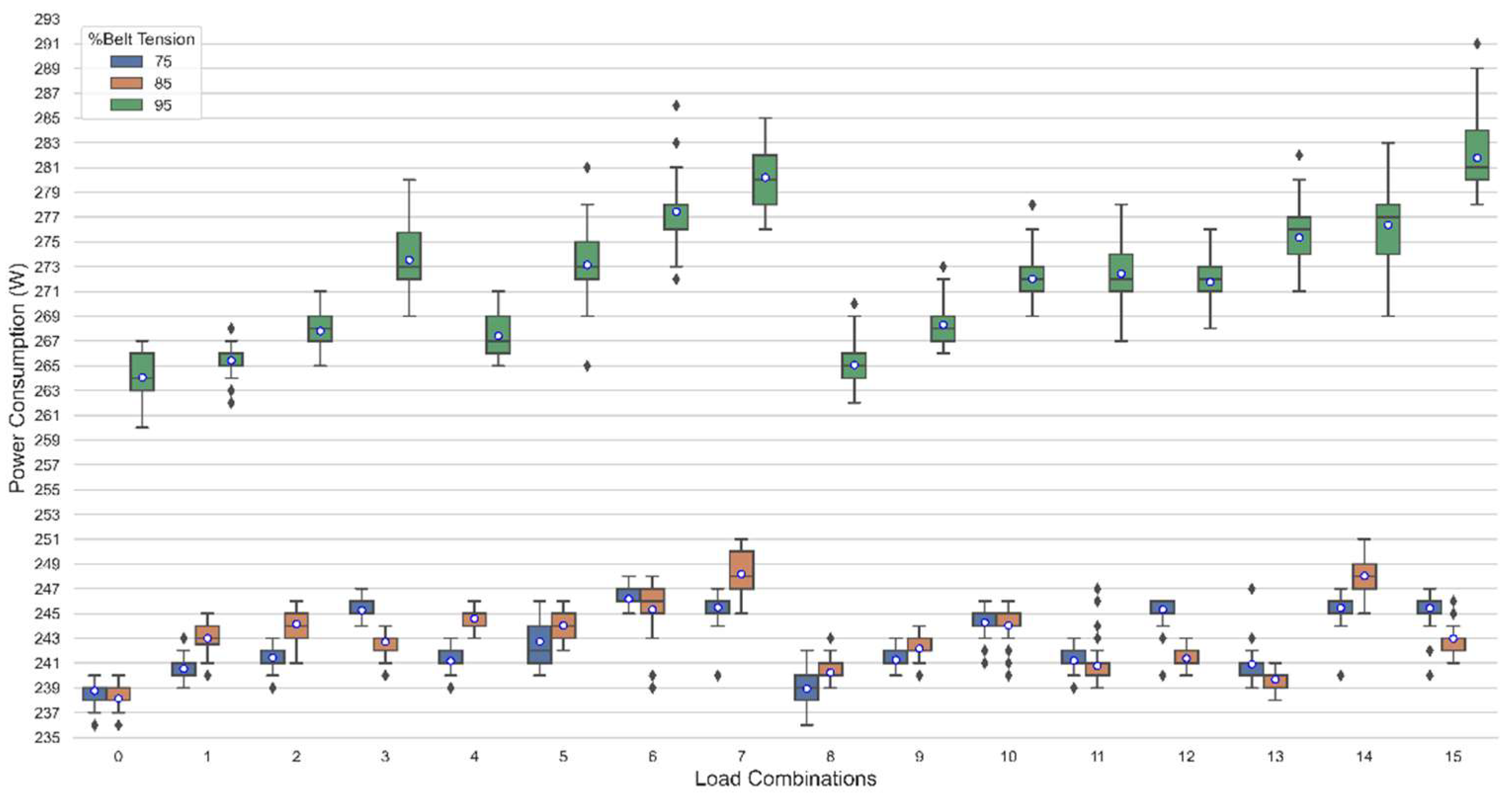Figure 9 shows the boxplot for 75% and 85% belt tensions, depicting the effect of the pallet positions and belt tensions on the conveyor belt motor driver’s power consumption.

Table 5. Dynamic case results for 75–85% belt tension with no active zones.

Belt Tension (%)	Act. Zone	Src. Zone	Dst. Zone	Distance (m)	Time (s)	Speed (m/s)
75	No	1	5	1.61	5.36	0.3
75	No	1	2	0.61	2.23	0.274
75	No	1	3	0.835	2.95	0.283
75	No	3	5	0.773	2.97	0.26
85	No	1	5	1.61	5	0.322
85	No	1	2	0.61	2.18	0.28
85	No	1	3	0.835	2.84	0.294
85	No	3	5	0.773	2.78	0.278

and

Table 6. Dynamic case results for 75–85% belt tension with active zones.

Belt Tension (%)	Act. Zone	Src. Zone	Dst. Zone	Distance (m)	Time (s)	Speed (m/s)
75	Z5	1	3	0.835	2.91	0.287
75	Z5, Z3	1	2	0.61	2.29	0.266
75	Z1, Z2	3	5	0.773	4.24	0.182
75	Z1	2	3	0.223	1.2	0.186
85	Z5	1	3	0.835	2.85	0.293
85	Z5, Z3	1	2	0.61	2.07	0.295
85	Z1, Z2	3	5	0.773	2.89	0.267
85	Z1	2	3	0.223	1.02	0.219

show the dynamic case results for these belt tensions with and without active zones. It was observed that with 85% belt tension, it took 5 s for a pallet to move from Z1 to Z5. On the other hand, it took 5.36 s for a pallet to move from Z1 to Z5 with 75% belt tension. One significant observation noticed for the 75% belt tension was that it took 4.24 s for a pallet to move from Z3 to Z5 when two zones were active (i.e., Z1 and Z2). This was due to the increase in friction along the conveyance path and belt slippage at the head pulley. This meant a reduction in the required necessary frictional driving force between the motor driver head pulley (driving wheel) and the conveyor belt, and this led to a situation where the load movement was not as smooth as in other combinations. Besides that, there was no significant difference between the dynamic case results of these belt tensions and no belt slippage, and mistracking was observed for these belt tensions as observed for the 70% belt tension.

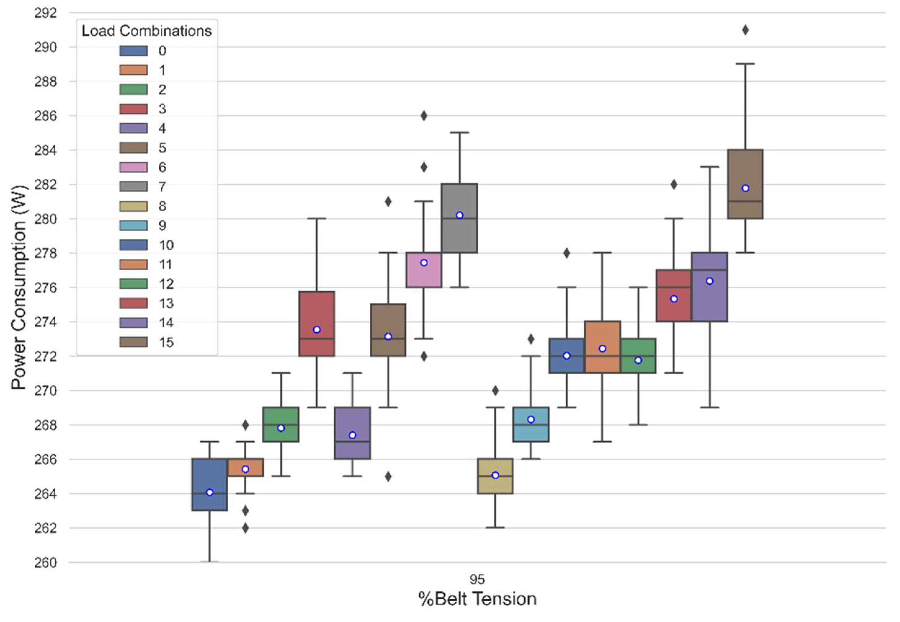
5.3. Results and Analysis for 95% Belt Tension

For this belt tension, a better, smoother belt motion was observed and there was no slip at the head pulley. Figure 10 shows how the conveyor motor driver power consumption was affected by the belt tension, as well as the presence of load on different zones of the conveyor at a time. For this belt tension, a significant increase in power consumption was observed for all combinations. This was the maximum achievable belt tension. This belt tension induced excessive stress on the belt, motor bearings and shafts, and so the motor drew more current to produce enough torque to maintain a smooth belt motion. This is an unhealthy operation, which is harmful to the belt, motor shaft and bearings. This extra stress can also cause the pulleys to break and wear down prematurely. Tracking problems can also arise, leading to uneven belt wear. Similar to belt tensions 75% and 85%, the experiment was conducted for all load combinations.

Table 7. Dynamic case results for 95% belt tension without active zones.

Belt Tension (%)	Act. Zone	Src. Zone	Dst. Zone	Distance (m)	Time (s)	Speed (m/s)
95	No	1	5	1.61	4.6	0.35
95	No	1	2	0.61	1.98	0.308
95	No	1	3	0.835	2.86	0.292
95	No	3	5	0.773	2.77	0.279

and

Table 8. Dynamic case results for 95% belt tension with active zones.

Belt Tension (%)	Act. Zone	Src. Zone	Dst. Zone	Distance (m)	Time (s)	Speed (m/s)
95	Z5	1	3	0.835	2.85	0.293
95	Z5, Z3	1	2	0.61	1.99	0.307
95	Z1, Z2	3	5	0.773	2.8	0.276
95	Z1	2	3	0.223	1.02	0.219

show the dynamic case results for 95% belt tension with and without active zones. The dynamic case results for this belt tension were better than the dynamic case results obtained for 75% and 85% belt tensions. For 95% belt tension, it took 4.6 s for a pallet to move from Z1 to Z5.

5.4. Comparison Plots for Belt Tensions

For 95% belt tension, a minimum power consumption of 259.5 W was recorded for load combination 0 (no load) as compared to previous belt tensions (0% to 85%), which was greater than the maximum power consumption of 251 W recorded at 85% belt tension for load combinations 3, 7, 14 and 15. Figure 11 shows the comparison boxplots for 75% to 95% belt tensions. For 75% to 95% belt tensions, the conveyor belt motor driver power consumption varied between 235 W and 289 W, and for the 75% and 85% belt tensions, the power consumption varied from 235 W to 251 W. As mentioned earlier, 95% was the maximum belt tension that could be achieved in the conveyor belt, and any operation with this belt tension is harmful for both the motor and the belt and must be avoided.

Similarly, Figure 12 shows comparison boxplots for 0% to 85% belt tensions. From the analysis presented in the previous section, for the 0% to 70% belt tensions, the conveyor belt parameters remained the same irrespective of the fact that for the 70% belt tension there was motion in the conveyor belt under the no load condition, but as soon as there was a pallet at Z1, the belt slip at the head pulley increased and the power consumption dropped to 232.2 W (data mean), hence, leaving no separation boundary between the 60% and 70% belt tensions. Therefore, all belt tension values which were less than or equal to 70% were treated as not useful belt tension values.

Based on the data analysis and the results described in the previous sections, the data collected could be classified into three distinct belt tension classes, namely, “low”, “optimal” and “over-tensed” (Figure 13). Each box plot in Figure 13 represents the power consumed by the conveyor belt motor driver for all load combinations corresponding to the belt tension. From the analysis of static and dynamic data, it was observed that the conveyor belt started moving without any load at 70% belt tension and showed a jerky motion when the pallet moved from Z1 to Z5 (marked as dark yellow in the figure). In contrast, at 95% belt tension, no jerks or belt slippage were observed, but the belt stretch and stress on the motor bearing were much higher than other belt tensions, and even a belt tension squeal sound was audible (marked as red in the figure). The belt tension values which were in between these two extremes showed moderate results, hence; 70% belt tension was the lower threshold, and 95% belt tension was the upper threshold (marked as green in the figure). The belt tension had to be set between these two thresholds for optimal transportation operations.

5.5. Model Training and Prediction Results

The prognostic model, which was an artificial neural network, was trained using the static case data with the aim of predicting an early-stage behavioural deterioration of conveyor belts. The developed model was used for multiclass classification to predict a belt tension class Cm, where m was 1, 2 or 3, which represented low, optimal and over-tensed belt tension classes (

Table 9. Belt tension classes correlating to % belt tension values.

Class	Belt Tension Values in %	Description
1	0% to 70%	Not useful (low)
2	75% to 85%	Useful (optimal)
3	Belt tension > 90%	Not useful (over-tensed)

).

The static case data included more than 4500 data samples collected from the FASTory line at a sampling rate of 1 s, and out of these samples, 80% was used for model training, 10% of samples was used for validation and the remaining 10% of data samples was used for testing the model. The computed loss/error, i.e., the average percentage of the number of unsuccessful predicted classes, was 3.2%. This misclassification error was observed for only those data samples that corresponded to the “no-load” situation, i.e., load combination 0 for belt tensions 70%, 75% and 85% due to data overlapping and a low separation boundary. Another reason for this error was that the conveyor power consumption did not change instantly once the conveyor load was modified, but only after a short time delay. This delay was responsible for the few outliers, and such occurrences may have influenced the value of the calculated error. Figure 14 illustrates the data overlapping with box plots for load combinations 0 and 1 with a belt tension range from 0% to 85%.

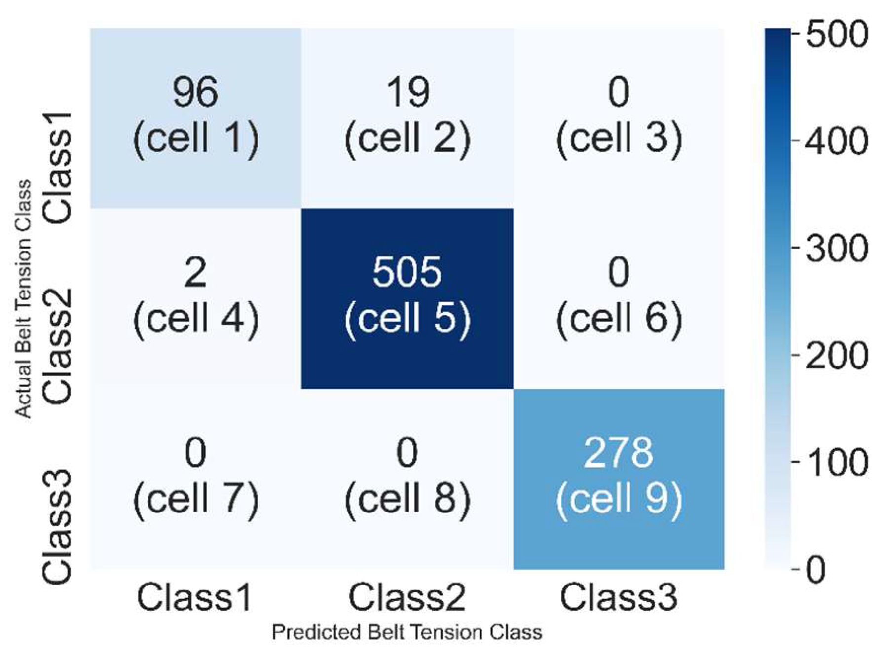
After testing, the model was used for the prediction of real-time data coming from the FASTory line, and prediction results went according to expectations. During the real-time prediction, both belt tensions and loads were varied by the line operator according to Table 2 and Table 3, respectively. Similar to the test data, the same misprediction was observed for the real-time data. To assess the performance of the developed model, a confusion matrix providing a comparison between the actual and predicted belt tension class was used. The confusion matrix was N × N matrix, where N is the number of outputs of classes. In our case, there were three classes and, therefore, a 3 × 3 matrix. Figure 15 shows the confusion matrix of the developed prognostic model. The true positive, false positive, true negative and false negative values could be calculated from the model’s confusion matrix.

The true positive (TP), false positive (FP), true negative (TN) and false negative (FN) values were calculated as follows, and as presented in

Table 10. TP, FP, TN and FN values of ANN model.

Belt Tension Class	True Positive	False Positive	True Negative	False Negative
Class 1	96 (cell 1)	2 (cell 4 + 7)	783 (cell 5 + 6 + 8 + 9)	19 (cell 2 + 3)
Class 2	505 (cell 5)	19 (cell 2 + 8)	374 (cell 1 + 3 + 7 + 9)	2 (cell 4 + 6)
Class 3	278 (cell 9)	0 (cell 3 + 6)	622 (cell 1 + 2 + 4 + 5)	0 (cell 7 + 8)

:

• TP: The true positive value was where the actual belt tension class and predicted belt tension class were the same;
• FP: The false positive value for a belt tension class was the sum of values of the corresponding column, except for the TP value;
• TN: The true negative value for a belt tension class was the sum of values of all columns and rows, except for the values of that class being calculated;
• FN: The false negative value for a belt tension class was the sum of values of corresponding rows, except for the TP values.

6. Conclusions and Future Work

This paper presented an approach that used the power signature from the conveyor belt driver to describe the expected system behaviour. In summary, the power consumption values of a conveyor belt-based transportation system in a discrete production system were monitored and classified for a real factory automation testbed. During the training phase, the power signature of the system components and workload of the conveyor belts was associated with semantics concerning the conveyor belt tension, and in the validation phase, real-time data coming from the line served as the input to the predictor model, which predicted the belt tension class. Consecutive mismatches between the latest and the last 10 predicted belt tension classes implied a gradual deterioration of belt tension from the optimal belt tension range, which pointed to an incipient gradual deterioration of expected behaviour of the equipment. In the presented scenario, such a deterioration would translate to a gradual loss of conveyor belt tension, and maintenance steps would have to be taken for the equipment to avoid causing catastrophic hazards. Future research should focus on introducing more parameters for the analysis and increasing the number of dimensions of the available datasets, for instance, by installing vibration and temperature sensors for the conveyor belt motor driver.

References

- Mohammed, W.M.; Ferrer, B.R.; Iarovyi, S.; Negri, E.; Fumagalli, L.; Lobov, A.; Lastra, J.L.M. Generic platform for manufacturing execution system functions in knowledge-driven manufacturing systems. Int. J. Comput. Integr. Manuf. 2018, 31, 262–274. [Google Scholar] [CrossRef]
- Khajehzadeh, N.; Postelnicu, C.; Lastra, J.L.M. Detection of abnormal energy patterns pointing to gradual conveyor misalignment in a factory automation testbed. In Proceedings of the IEEE International Conference on Systems, Man, and Cybernetics (SMC), Seoul, Korea, 14–17 October 2012. [Google Scholar] [CrossRef]
- Wang, H.; Chai, T.-Y.; Ding, J.-L.; Brown, M. Data driven fault diagnosis and fault tolerant control: Some advances and possible new directions. Acta Autom. Sin. 2009, 35, 739–747. [Google Scholar] [CrossRef] [Green Version]
- Mobley, R.K. An Introduction to Predictive Maintenance, 2nd ed.; Elsevier: Amsterdam, The Netherlands, 2002. [Google Scholar]
- Kawalec, W.; Suchorab, N.; Konieczna-Fuławka, M.; Król, R. Specific energy consumption of a belt conveyor system in a continuous surface mine. Energies 2020, 13, 5214. [Google Scholar] [CrossRef]
- Faltinski, S.; Flatt, H.; Pethig, F.; Kroll, B.; Vodencarevic, A.; Maier, A.; Niggemann, O. Detecting anomalous energy consumptions in distributed manufacturing systems. In Proceedings of the 10th International Conference on Industrial Informatics, Beijing, China, 25–27 July 2012. [Google Scholar] [CrossRef]
- Niebel, B.W. Engineering Maintenance Management, 2nd ed.; Marcel Dekker: New York, NY, USA, 1994. [Google Scholar]
- Gutschi, C.; Furian, N.; Suschnigg, J.; Neubacher, D.; Voessner, S. Log-based predictive maintenance in discrete parts manufacturing. Procedia CIRP 2019, 79, 528–533. [Google Scholar] [CrossRef]
- Tsang, A.H.C. Condition-based maintenance: Tools and decision making. J. Qual. Maint. Eng. 1995, 1, 3–17. [Google Scholar] [CrossRef]
- Samatas, G.G.; Moumgiakmas, S.S.; Papakostas, G.A. Predictive maintenance—Bridging artificial intelligence and IoT. In Proceedings of the IEEE World AI IoT Congress (AIIoT), Seattle, WA, USA, 10–13 May 2021. [Google Scholar] [CrossRef]
- Swanson, L. Linking maintenance strategies to performance. Int. J. Prod. Econ. 2001, 70, 237–244. [Google Scholar] [CrossRef]
- Gits, C.W. Design of maintenance concepts. Int. J. Prod. Econ. 1992, 24, 217–226. [Google Scholar] [CrossRef] [Green Version]
- Zhang, J.; Tu, Y.; Yeung, E.H.H. Intelligent decision support system for equipment diagnosis and maintenance management. In Proceedings of the Innovation in Technology Management. The Key to Global Leadership, PICMET ’97, Portland, OR, USA, 31 July 1997. [Google Scholar] [CrossRef]
- Rødseth, H.; Schjølberg, P. Data-driven predictive maintenance for green manufacturing. In Proceedings of the 6th International Workshop of Advanced Manufacturing and Automation, Manchester, UK, 10–11 November 2016. [Google Scholar] [CrossRef] [Green Version]
- Venkatasubramanian, V.; Rengaswamy, R.; Kavuri, S.N.; Yin, K. A review of process fault detection and diagnosis: Part III: Process history based methods. Comput. Chem. Eng. 2003, 27, 327–346. [Google Scholar] [CrossRef]
- Frank, P.M. Analytical and qualitative model-based fault diagnosis—A survey and some new results. Eur. J. Control 1996, 2, 6–28. [Google Scholar] [CrossRef]
- Yam, R.C.M.; Tse, P.; Li, L.; Tu, P. Intelligent predictive decision support system for condition-based maintenance. Int. J. Adv. Manuf. Technol. 2001, 17, 383–391. [Google Scholar] [CrossRef]
- Hashemian, H.M. State-of-the-art predictive maintenance techniques. IEEE Trans. Instrum. Meas. 2011, 60, 226–236. [Google Scholar] [CrossRef]
- Wu, S.-J.; Gebraeel, N.; Lawley, M.A.; Yih, Y. A neural network integrated decision support system for condition-based optimal predictive maintenance policy. IEEE Trans. Syst. Man Cybern. Part A Syst. Hum. 2007, 37, 226–236. [Google Scholar] [CrossRef]
- Rosebrock, A. A simple neural network with Python and Keras. Deep Learning, Machine Learning. 2016. Available online: pyimagesearch.com/2016/09/26/a-simple-neural-network-with-python-and-keras/ (accessed on 30 March 2022).
- Namuduri, S.; Narayanan, B.N.; Davuluru, V.S.P.; Burton, L.; Bhansali, S. Review—Deep learning methods for sensor based predictive maintenance and future perspectives for electrochemical sensors. J. Electrochem. Soc. 2020, 167, 37552. [Google Scholar] [CrossRef]
- Goodfellow, I.; Bengio, Y.; Courville, A. Deep Learning; MIT Press: Cambridge, MA, USA, 2016. [Google Scholar]
- LeCun, Y.; Bengio, Y.; Hinton, G. Deep learning. Nature 2015, 521, 436–444. [Google Scholar] [CrossRef] [PubMed]
- Hopfield, J.J. Neural networks and physical systems with emergent collective computational abilities. Proc. Natl. Acad. Sci. USA 1982, 79, 2554. [Google Scholar] [CrossRef] [PubMed] [Green Version]
- Luxhøj, J. An artificial neural network for nonlinear estimation of the turbine flow-meter coefficient. Eng. Appl. Artif. Intell. 1998, 11, 723–734. [Google Scholar] [CrossRef]
- Shao, J. Application of an artificial neural network to improve short-term road ice forecasts. Expert Syst. Appl. 1998, 14, 471–482. [Google Scholar] [CrossRef]
- Iarovyi, S.; Mohammed, W.M.; Lobov, A.; Ferrer, B.R.; Lastra, J.L.M. Cyber–physical systems for open-knowledge-driven manufacturing execution systems. Proc. IEEE 2016, 104, 1142–1154. [Google Scholar] [CrossRef]
- INICO Tech. Available online: https://www.inicotech.com/s1000_overview.html (accessed on 30 March 2022).
- DIN 22101—2011—Belt Conveyors. Available online: https://www.scribd.com/document/293857373/DIN-22101-2011-Belt-Conveyors (accessed on 30 March 2022).
- Cema. Belt tension, power, and drive engineering. In Cema Belt Book; CEMA, 6th ed.; CEMA: Naples, Italy, 2005. [Google Scholar]
Figure 1.
Taxonomy of predictive maintenance [
14].
Figure 2.
A simple ANN with two hidden layers [
20].
Figure 3.
FASTory production assembly line [
27].
Figure 4.
FASTory line layout [
Figure 5.
Power consumption monitoring in the testbench [
2].
Figure 6.
Motor driver with head pulley at main conveyor.
Figure 7.
Main steps for development of the data-driven prognostic model.
Figure 8.
Effect of belt tensions (0–70%) and load on conveyor motor driver power consumption.
Figure 9.
Effect of belt tension (75–85%) and load on conveyor motor driver power consumption.
Figure 10.
Effect of 95% belt tension and load on conveyor motor driver power consumption.
Figure 11.
Comparison of 75%, 85% and 95% belt tensions.
Figure 12.
Comparison of 0–85% belt tensions.
Figure 13.
Power consumption of the conveyor belt motor driver for all load combinations corresponding to the belt tension.
Figure 14.
Data overlapping (misprediction).
Figure 15.
Confusion matrix of FASTory belt tension class predictor ANN model.