Article

One-Day-Ahead Solar Irradiation and Windspeed Forecasting with Advanced Deep Learning Techniques

by
Konstantinos Blazakis
1,*,
Yiannis Katsigiannis
2 and
Georgios Stavrakakis
1
1
School of Electrical and Computer Engineering, Technical University of Crete, GR-73100 Chania, Greece
2
Department of Electrical and Computer Engineering, Hellenic Mediterranean University, GR-71004 Heraklion, Greece
*
Author to whom correspondence should be addressed.
Energies 2022, 15(12), 4361; https://doi.org/10.3390/en15124361
Submission received: 30 April 2022 / Revised: 6 June 2022 / Accepted: 9 June 2022 / Published: 15 June 2022

Abstract

:
In recent years, demand for electric energy has steadily increased; therefore, the integration of renewable energy sources (RES) at a large scale into power systems is a major concern. Wind and solar energy are among the most widely used alternative sources of energy. However, there is intense variability both in solar irradiation and even more in windspeed, which causes solar and wind power generation to fluctuate highly. As a result, the penetration of RES technologies into electricity networks is a difficult task. Therefore, more accurate solar irradiation and windspeed one-day-ahead forecasting is crucial for safe and reliable operation of electrical systems, the management of RES power plants, and the supply of high-quality electric power at the lowest possible cost. Clouds’ influence on solar irradiation forecasting, data categorization per month for successive years due to the similarity of patterns of solar irradiation per month during the year, and relative seasonal similarity of windspeed patterns have not been taken into consideration in previous work. In this study, three deep learning techniques, i.e., multi-head CNN, multi-channel CNN, and encoder–decoder LSTM, were adopted for medium-term windspeed and solar irradiance forecasting based on a real-time measurement dataset and were compared with two well-known conventional methods, i.e., RegARMA and NARX. Utilization of a walk-forward validation forecast strategy was combined, firstly with a recursive multistep forecast strategy and secondly with a multiple-output forecast strategy, using a specific cloud index introduced for the first time. Moreover, the similarity of patterns of solar irradiation per month during the year and the relative seasonal similarity of windspeed patterns in a timeseries measurements dataset for several successive years demonstrates that they contribute to very high one-day-ahead windspeed and solar irradiation forecasting performance.

Graphical Abstract

1. Introduction

A significant amount of global and domestic energy requirements are covered by fossil fuel consumption. It is widely accepted that consuming fossil fuels such as oil, coal, and natural gas releases a large amount of greenhouse gasses into the atmosphere, leading to extremely negative effects on the environment. The production of “cleaner”, carbon-free energy can be achieved by utilizing renewable energy sources such as the wind and sun, which have begun to be used to cover the globe’s increasing energy needs. Electric energy market liberalization in conjunction with the increasing need for sustainable energy has turned political and investing interests into further utilizing RES to cover electricity needs [1,2].
Energy produced from the wind and the sun depends largely on local weather conditions, such as temperature, windspeed, air pressure, humidity, sunlight, etc., and their fluctuations. Thus, wind and solar power generation is often difficult to control and predict, as weather conditions constantly change. This makes integration of wind and solar energy into power grids, especially isolated grids, a significant challenge [3,4].
To tackle the aforementioned challenge, it is essential to improve the performance of windspeed and solar irradiation one-day-ahead forecasting in order to minimize uncertainty about the amount of renewable power that can be generated in any electric grid operational situation. Given the inherent relationship between solar irradiation and the electric power produced from photovoltaics, and between windspeed and wind turbine power generation, it is necessary to create computational models that will accurately predict solar irradiation and windspeed in medium- and/or short-term time scales [5,6,7,8,9,10,11].
Windspeed forecasting can be separated into four temporal ranges: very short-term (from a few seconds to 30 min), short-term (from 30 min to 6 h ahead), medium-term (from 6 h to 1 day ahead), and long-term (more than 1 day ahead) [6]. Solar irradiation forecasting can also be divided into four temporal ranges: very short-term (a few minutes to 1 h), short-term (1–4 h), medium-term (1 day ahead), and long-term (more than 1 day ahead) [7].
Over the last few years, various tools have been established to predict windspeed and solar irradiation. These tools can be separated into three main groups: (1) data-driven models, such as statistical models and machine learning models, which are the most prevalent tools used for predicting such timeseries; (2) physical models that use meteorological and topographical data; and (3) hybrid algorithms, which have found great success in a number of research areas [3,6,8].
Regarding data-driven models, statistical methods consist of autoregressive integrated moving average (ARIMA) [9,10,11], auto-regressive moving average (ARMA) [12,13,14], Lasso [15], and Markov models [16,17,18]. The most common machine learning methods are support vector machines (SVM) [19,20,21], feed forward neural networks (FFNN) [22], recurrent neural networks (RNN) [23,24,25], convolutional neural networks (CNN) [26,27], long short-term memory networks (LSTM) [28,29,30,31], bidirectional long short-term memory neural networks (BiLSTM) [32], deep belief networks (DBN) [33], and artificial neural networks in general (ANN) [34,35,36].
Physical methods include numerical weather prediction (NWP) forecasting models [37,38], total sky imagery (TSI) [39], cloud-moving-based satellite imagery models [40], and weather research and forecasting (WRF) models [41].
Hybrid methods found in the literature include variational mode decomposition with Gram–Schmidt orthogonal and extreme learning machines, which are enhanced at the same time by a gravitational search algorithm [42], nonlinear neural network architectural models combined with a modified firefly algorithm and particle swarm optimization (PSO) [43], the hybrid model decomposition (HMD) method and online sequential outlier robust extreme learning machine (OSORELM) [44], empirical mode decomposition and Elman neural networks (EMD-ENN) [45], wavelet transform (WT-ARIMA) [46], empirical wavelet transform (EWT) and least-square support vector machines (LSSVM) improved by coupled simulated annealing [47], and variational mode decomposition (VMD) combined with several ML methods, including SVM and back propagation neural networks (BPNN). Moreover, ELMs and ENNs were implemented to perform advanced data preprocessing based on complementary ensemble empirical mode decomposition (CEEMD) [48], while sample entropy and VMD forecasting methods based on ENNs and on a multi-objective “satin bowerbird” optimization algorithm have been introduced [49]. Bidirectional long short-term memory neural networks with an effective hierarchical evolutionary decomposition technique and an improved generalized normal distribution optimization algorithm for hyperparameter tuning, a combined model system including an improved hybrid timeseries decomposition strategy (HTD), a novel multi-objective binary backtracking search algorithm (MOBBSA), and an advanced sequence-to-sequence (Seq2Seq) predictor for windspeed forecasting have been presented in [50,51], respectively. Further, recurrent neural network prediction algorithms combined with error decomposition correction methods have also been presented in [52].
The purpose of this paper is to develop models for high-performance, medium-term forecasting (i.e., for the next 24 h) of windspeed and solar irradiation, which will be based on hourly data recorded on Dia Island, which is located north of Heraklion city in Crete, Greece. In order to achieve this, the efficacies of three deep learning techniques, i.e., multi-channel CNN, multi-head CNN, and encoder–decoder LSTM, are investigated and compared with two conventional methods, i.e., RegARMA and NARX, in order, among other things, to demonstrate the improved forecasting performance of the deep learning techniques and to highlight the most effective among them. All the presented methodologies were tested on a benchmarked dataset of real measurements for the purpose of predicting with the highest possible statistical accuracy the windspeed and solar irradiation for a forecasting period of 24 h, i.e., of one day ahead.
The main contributions of this paper are:
  • A series of experiments applying advanced deep-learning-based forecasting techniques were conducted, achieving high statistical accuracy forecasts.
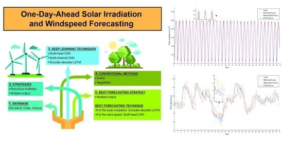
  • A thorough comparison is conducted successfully among advanced deep learning techniques and well-known conventional techniques for medium-term solar irradiance and windspeed forecasting to highlight the most effective among them.
  • A cloud index per hour (NDD(h,d)) was introduced and used for the first time in order to improve medium-term solar irradiance forecasting.
  • Data were categorized by each month for successive years, firstly due to the similarity of patterns of solar irradiation by month during the year, and secondly because of the relative seasonal similarity of the windspeed patterns, resulting in a monthly timeseries dataset, which is more significant for high-performance forecasting.
  • A walk-forward validation forecast strategy in combination first with a recursive multistep forecast strategy and secondly with a multiple-output forecast strategy was successfully implemented in order to significantly improve medium-term windspeed and solar irradiation forecasts.
  • The recursive multistep forecast strategy was compared to the multiple-output forecast strategy.
The paper is organized as follows: In Section 2, we present the theory behind the proposed deep learning forecasting methods and the real measurements categorized by each months’ dataset, model configurations, the methodology followed, and the algorithms for the medium-term windspeed and solar irradiation forecasting. In Section 3, the simulation results and the discussion of these results are presented, while in Section 4, the conclusions of the paper are summarized.

2. The Proposed Deep Learning Model Framework

2.1. Dataset Presentation

The dataset used in this research is derived from measurements carried out on Dia Island, Crete, Greece. Table 1 includes the required parameters given in hourly values for every day for years 2005–2016 at a height of 10 m from the ground. All these parameters were recorded except for the beam/direct irradiance on a plane always normal to the sun’s rays and the diffuse irradiance on the horizontal plane, which were estimated from the global irradiance on the horizontal plane using the anisotropic model described in [53]. The beam/direct irradiance on a plane always normal to the sun rays was considered for two main reasons: (1) it improves the forecasting performance of the examined models, and (2) it is an essential parameter for the estimation of a photovoltaic system’s performance in a specific location. Moreover, extraterrestrial irradiation is calculated using the typical solar geometry equations presented in [54]. Table 2 includes some statistical data for solar irradiation and windspeed, including maximum and minimum mean values and standard deviations (Std).
For solar irradiation forecasting, due to the lack of a cloud index, the normalized discrete index for each day (NDD(d)) and for each hour of the day (NDD(h,d)) were introduced and calculated by Equations (1) and (2) below, provided the extraterrestrial solar irradiation for Dia Island and the solar irradiation in the horizontal plane [36]. Due to the periodicity of solar irradiation, we constructed two columns: (1) the number of days in the month (31, 30 or 28); and (2) the hour of the day for every observation (1–24). For solar irradiation forecasting, the following parameters were used as inputs from the initial measurements’ dataset: air temperature, NDD(d), NDD(h,d), the number of days in the month, and the hour of the day. From the initial dataset of measurements, the nighttime values (zero solar irradiation) were removed due to the fact that night hours do not contribute to solar irradiation forecasting.
The parameters NDD(d) and NDD(h,d) are calculated as follows:
N D D ( d ) = 1 24 i = 1 24 ( G o n , d ( i ) G s n , d ( i ) ) 2
N D D ( h , d ) = G o n , h , d G s n , h , d
where “ d ” is the day of the year (1 to 365), “ i ” is the hour number of each day (1 to 24), “ h ” is the specific hour of the day for which the cloud index N D D ( h , d ) is calculated, G o n is the normalized extraterrestrial irradiance, and G s n is the normalized surface irradiance. Global irradiance data on the horizontal plane are presented in Table 1, where extraterrestrial irradiance data were calculated from well-known solar geometry equations, using as parameters the solar constant (1367 W/m2), day of the year, latitude and longitude of the location, solar hour angle, and declination angle of the Sun [54]. For normalization of G o n and G s n , their corresponding maximum values for each year of the dataset were used. Even if the value of extraterrestrial or surface irradiance exceeds its historical maximum (so the normalized maximum irradiance could slightly exceed 1), this does not affect the performance of the forecasting.
In addition, statistical parameters such as the maxima, minima, means, and standard deviations for windspeed and solar irradiation data are shown in Table 2.
For windspeed forecasting, the following parameters were used as inputs from the initial dataset: air temperature (°C), relative humidity (%), and global irradiance on the horizontal plane (W/m2) [5].

2.2. Presentation of the Proposed Deep Learning Models

2.2.1. Multi-Channel and Multi-Head CNNs

Convolutional neural networks (CNNs) are a category of artificial deep neural networks that are mainly used for image and video recognition, recommender systems, image and text classification, image analysis, facial recognition, document analysis, natural language processing, financial timeseries data, etc. [27,28,29].
A typical CNN consists of at least one convolutional layer, fully connected layers, flattened layers, pooling layers, and dropout layers. The purpose of the convolutional layer is to convolve the input image and generate the feature maps. Input image convolving is carried out by sliding a group of small-sized filters (kernels)—each of which contain a sufficient number of learnable weights—over the input image, implementing element-wise multiplication at each possible position. A completely new layer is generated from each kernel, which contains the application results of the particular kernel in the input image. The number of generated feature maps (convolutional layer depth) is defined by the number of kernels and constitutes the CNN hyperparameters, which must be chosen correctly based on available data. Then, this resulting group of layers undergoes a pooling process. Pooling involves a down-sampling operation in which sets of elements in the feature maps are integrated and restricted to a single value based on some criterion or calculation (e.g., maximum value or average of all values). As a result, noise data are eliminated, and better performance is achieved. Repeating the two aforementioned layers multiple times by applying different kernels of different sizes and depths, successive extraction of higher-level features improves, which constitutes one of the assets of CNNs. Dropout layers can be used after convolutional layers and pooling layers to protect neural networks from overfitting.
Finally, the last pooled layer can be converted into a single vector that includes all of its weights and which is connected to a fully connected layer, which is further connected to the output layer that contains a summation of every possible class, thus providing the classification success estimation for the given input [55,56,57,58].
The multi-channel approach applied in this paper is based on the aforementioned typical CNN architecture and extends it by adding a further embedding layer into the model in order to raise the number of channels matching the degree of semantic enrichment of the present paper’s data. Multi-channel CNNs use each of the solar irradiation inputs and the windspeed forecasting timeseries variables to predict the windspeed and solar irradiation of the next day. This is implemented by entering each one-dimensional timeseries into the model as a separate input channel. A distinct kernel is then used by the CNN, which will read each input sequence onto a separate set of filter maps, essentially learning features from each input timeseries variable. This is useful for situations where the output sequence is some function of the observations at prior timesteps derived from their multiple different features, and also when the output sequence does not contain only the feature to be forecasted [57,59].
Another extension of the CNN model is to obtain a separate sub-CNN model, or, in other words, a head for each input variable, whose structure can be referred to as a multi-headed CNN model. This extension requires transformation of the model preparation, and, in turn, modification of the preparation of the training and test datasets. Regarding the model, a separate CNN model must be defined for each of the input variables: solar irradiation and windspeed. Inserting each input into an independent CNN has a number of advantages, such as feature extraction that is improved by focusing only on one input, and each convolutional head can be controlled for the specific nature of each input. The configuration of the model, taking into consideration the number of layers and their hyperparameters, was also modified to better suit the new approach presented above [57].

2.2.2. Encoder–Decoder LSTM

Long short-term memory (LSTM) is a modified version of artificial recurrent neural network (RNN) architecture mainly used in deep learning algorithms. LSTMs use feedback connections, in contrast to standard feed forward neural networks, which enhances the memory recovery of a given network. LSTMs can process single data points (such as images) and entire sequences of data (such as speech or video); therefore, LSTMs are suitable for applications such as unsegmented, connected handwriting recognition, speech recognition, anomaly detection in network traffic or intrusion detection systems (IDSs), etc. [60].
A common LSTM unit consists of a cell, an input gate (to investigate which information should be used for memory modification), an output gate, and a forget gate (to decide the information to be dismissed). The cell remembers values over arbitrary time intervals, and the three gates adjust the information flow into and out of the cell.
LSTM networks are appropriate for forecasting, classifying, and processing based on timeseries data, since unknown duration lags may exist between important events when dealing with timeseries problems. LSTMs are able to cope with the vanishing gradient problem that can arise during training of traditional RNNs. Their relative insensitivity to gap lengths is an advantage of LSTMs over RNNs, hidden Markov models, and other sequence learning methods in numerous applications [61].
Encoder–decoder LSTM is a recurrent neural network designed to cope with sequence-to-sequence (seq2seq) problems (text translation, learning program execution, etc.). Due to variations in the number of items in the inputs and outputs, sequence-to-sequence prediction problems have been worth studying. One advantage of an encoder–decoder LSTM is its use of fixed-sized internal representation in the core of the model [59].
The encoder and the decoder are usually LSTM units or gated recurrent units. The purpose of the encoder is to read the input sequence and to summarize the information in the internal state vectors (the hidden state and cell state vectors in the case of LSTMs). The outputs of the encoder can be discarded; only the internal states need to be retained. The decoder is an LSTM whose initial states are initialized to the final states of the encoder LSTM. Using these initial states, the decoder starts to generate the output sequence (see Figure 1).
The decoder operates slightly differently during training and inference. During training, teacher forcing is used, which accelerates decoder training. The input to the decoder at each timestep is the output from the previous timestep.
The encoder transforms the input sequence into state vectors (known as thought vectors), which are then inserted into the decoder in order to start output sequence generation according to the thought vectors. The decoder is just a language model conditioned by the initial states [61].

2.3. Solar and Wind Data Preprocessing and Forecasting Model Configurations

To appropriately train the model, two data preprocessing procedures were carried out. The first procedure normalized the data and the latter procedure accommodated for missing data. As for the latter, the average of nearby values during the same week was calculated to fill missing data values. Furthermore, it is worth noting that data normalization before inserting the input data into the network is a good practice, since inserting variables with both large and small magnitudes will have negative effects on learning algorithm performance. For data normalization, the well-known formula of Equation (3) was used:
y = x i x m i n x m a x x m i n
where y is the normalized value, x i is the current value, and x m i n and x m a x are the minimum and the maximum of the original parameters, respectively.
These data were categorized by month, resulting in a monthly timeseries for years 2005–2016, which was then followed by model training and medium-term forecasting. Data were separated by month mainly because of the similarity of solar irradiation patterns, and secondly because of the relative similarity of windspeed patterns.
The most commonly used strategies for making multistep forecasts are [6,28,30,62]:
1.
Direct Multistep Forecast Strategy.
For every timestep forecast, a new model is developed. This strategy demands large computational time since there are as many models to learn as the size of the forecasting horizon.
2.
Recursive Multistep Forecast Strategy.
The recursive multistep strategy first trains a one-step model and then uses this single model for each horizon, but the prediction of the prior timestep is used as an input in place of the original dataset value for making a prediction at the following timestep. The recursive approach is not so computationally intensive in comparison with the direct strategy, as only one model is fitted. This type of strategy strengthens error accumulation because the predictions of prior steps are inserted into the model instead of the real values. This phenomenon results in poor algorithm performance as the prediction time horizon increases.
3.
Direct–Recursive Hybrid Multistep Forecast Strategy.
In this strategy, a combination of direct and recursive strategies is used in order to take advantage of both methods. This method computes the forecasts with different models for every forecasting horizon (direct strategy), and at each timestep it enlarges the set of inputs by adding variables corresponding to the forecasts of the previous step (recursive strategy).
4.
Multiple Output Forecast Strategy.
For the multiple output strategy, one model is developed in order to predict the whole forecast sequence in a one-shot manner.
In this study, the walk-forward validation forecast strategy is introduced, with an adaptive training window that expands after the desired forecast horizon (of 24 h) to include each time’s recent actual (measured) values, and was applied with improved success for a prediction horizon of 24 h. The walk-forward validation forecast strategy splits the monthly timeseries dataset into preconcerted sub-fragments. Walk-forward validation is based on the sliding window method, where the data are used in ascending order of time rather than randomly shuffling training–test datasets. This validation approach is essential for time-series analysis methods in general, where observations with future timestamp information cannot be used to predict past (old) values. Thus, it is crucial to assess model forecasting performance by recursively augmenting training data with recent observations and reevaluating the model over the extended horizon [62]. The recursive multistep forecast strategy and the multiple-output forecast strategy are applied over expanded timeseries fragments with a fixed sliding window of 24 h. The recursive multistep forecast strategy computes one-step-ahead forecasts (i.e., 1 h ahead) recursively until the desired forecast horizon (24 h) is achieved, while the multiple-output forecast strategy predicts the whole forecast horizon (i.e., 24 h ahead) in a one-shot manner. Then, the training set is expanded to incorporate recent actual (measured) values. Especially for solar irradiation forecasting, the sliding window magnitude is smaller than 24 h due to the subtraction of zero solar irradiation for every day, and it depends on the variable length of night during the year. Although the sliding window is smaller than 24 h (because of the excluded night hours), it represents, for the forecasting procedure, the window of the previous 24 h. For the training set, the months from the 2005–2014 monthly timeseries dataset were used in order to forecast the values for the corresponding months of 2015 and 2016. For instance, in order to forecast the windspeed and solar irradiation for January of 2015 and January of 2016, the measurements (dataset) for January in the years 2005–2014 were used to train the forecasting model. For every 24 h ahead forecasting, the real measurements (training dataset) available until midnight of the previous day were used to train the forecasting models [59].
The methodologies presented above for solar irradiation and windspeed medium-term forecasting with the recursive multistep forecast strategy and the multiple-output forecast strategy are described formally by the following equations, respectively:
ŷ (h, d) = f(ŷ(h − 1, d), …, ŷ(hk + 1, d), y(hk, d − 1), …, y(h − 24, d − 1), ui(h − 1, d − 1), ui(hk + 1, d − 1), ui(hk, d − 1), …, ui(h − 24, d − 1))
ŷ (h, d) = f(y(h − 1, d − 1), …, y(hk + 1, d − 1), y(hk, d − 1), …, y(h − 24, d − 1), ui(h − 1, d − 1), ui(hk + 1, d − 1), ui(hk, d − 1), …, ui(h − 24, d − 1))
where: “ŷ” is the predicted value for hour “h”, ….,“h − (k − 1) i.e., hk + 1” of day “d”; …y(hk, d − 1),…. y(h − 24, d − 1) are the historical measured values, “ui” represents the other external inputs (i.e., air temperature, relative humidity, global irradiance on the horizontal plane for windspeed forecasting, and air temperature), NDD(d), NDD(h,d) are the number of days in the month and the hour of the day, respectively, for solar irradiation forecasting, and k is the time instant sliding index.
In Table 3, the configuration of each layer for each model used is presented.
Concerning the data shapes of encoder–decoder LSTM, multi-channel CNN, and multi-head CNN, one sample consists of 24 timesteps (i.e., 24 h ahead), with three features for windspeed forecasting and five features for solar irradiation. The training dataset has 300 days (7200 h) or 310 days (7440 h) of data, so the shape of the training dataset would be: [7200/7440, 24, 3/5].
The encoder–decoder LSTM model consists of two sub-models, the encoder and the decoder. The purpose of the encoder is to read and encode the input sequence, and then the decoder reads the encoded input sequence and makes a one-step prediction for each element in the output sequence. After the input sequence reading by the encoder, a 200-element vector output is constructed (one output per unit) that captures features from the input sequence. At first, the internal representation of the input sequence is iterated multiple times, once for each timestep in the output sequence. This sequence of vectors is carried forward to the LSTM decoder. Then, the decoder is defined as an LSTM hidden layer with 200 units. It is worth mentioning that the decoder will output the entire sequence, not just the output at the end of the sequence, as was done with the encoder. This means that each of the 200 units will output a value for each of the 24 h, representing the basis of what to predict for each hour in the output sequence. Then, a fully connected layer to interpret each timestep in the output sequence is used before the final output layer. It is important to note that the output layer predicts a single step in the output sequence, not all of the 24 h at a time.
In multi-head CNN, a different CNN sub-model reads each input with two convolutional layers with 32 filters with a kernel size of 3, a max pooling layer, and a flattened layer. The internal representations come together before them to be interpreted by two fully connected layers of 200 and 100 nodes, respectively, and used to make a prediction.
In multi-channel CNN, a separate channel is linked to each input, similar to different image channels (e.g., red, green, and blue). A model that shows excellent performance consists of two convolutional layers with 32 filter maps with a kernel size of 3 followed by pooling, then another convolutional layer with 16 feature maps and pooling. The fully connected layer that interprets the features consists of 100 nodes.
The choice of hyperparameter values is of great importance [63,64,65,66]; for this reason, the well-known grid search method was adopted [49,67,68]. In this study, a grid search took place for the number of prior inputs, training epochs, and samples to include in each mini-batch, optimizer type, type of activation function, and learning rate. In more detail, for number of prior inputs, a set of {6, 12, 24, 48} was examined; for number of training epochs, a set of {5–100} was examined; for mini-batch size, a set of {8–512} was examined; optimizer types {RMSProp, ADAM, SGD, AdaGrad, AdaDelta, AdaMax, NADAM} were applied; activation functions {Relu, Elu, Tanh, Sigmoid} were applied; the learning rate takes values within {10−5–10−1}; see refs [49,67,68]. The grid search ended up with the optimal hyperparameters shown in Table 4.
In this research, 12 monthly models were applied for each deep learning technique for solar irradiation and windspeed one-day-ahead forecasting, and were developed with their corresponding optimal parameter configurations. Each model was run 20 times by performing several experiments in order to reduce the forecasting error statistics, which was found to be sufficient for the present work’s case studies. Then, the findings were recorded according to the mean values of the forecasting performance statistical metrics. Computations were carried out on a desktop computer with the following characteristics: 64 bit OS, CPU i5 2.30 GHz, and 8.00 GB of RAM. The forecasting run time for each test set was about 8 min.

3. Deep Learning and Conventional Forecasting Model Performance and Discussion

3.1. Deep Learning Forecasting Performance Evaluation Using Well-Established Error Metrics

Having arrived at the optimal hyperparameters of the forecasting models, evaluation of the results of windspeed and solar irradiation forecasting was based on well-known relationships to calculate the deviation (error) between predicted and real (measured) values, i.e., the well-known forecasting error statistical metrics [1]. These well-known relationships that are used extensively to evaluate forecasting methods in such prediction problems are shown in Table 5, where Y is the actual value and Y ^ is the forecasted value.
In Figure 2, Figure 3, Figure 4 and Figure 5, solar irradiation hourly predictions and windspeed hourly predictions are presented for July and November of 2016 for all the deep learning models that were applied in this survey. The figures followed with the letter ‘a’ (e.g., Figure 2a) refer to the recursive multistep forecast strategy, while the figures followed with the letter ‘b’ refer to the multiple-output forecast strategy. It is clarified that in Figure 2, Figure 3, Figure 4 and Figure 5 in the horizontal axes the time unit is ‘hour’, but obviously this is not possible to show graphically; thus, the time interval appearing is ‘day’, so within each interval of ‘one day’, 24 hourly values are depicted. The fluctuations in solar irradiation observed in Figure 3a,b are due to the cloudy weather during November, in contrast with Figure 2a,b, where the clear sky during July gives an almost periodical curve. In both Figure 4a,b and Figure 5a,b, small and high variations in the windspeed were observed.
The average daily performance metrics for each of the three deep learning algorithms applied for each month of 2015 and 2016 for solar irradiation forecasting and windspeed forecasting are presented in Table 6 and Table 7, respectively, in order to determine which method is more appropriate for solar irradiation and windspeed forecasting. In Table 6 and Table 7, CNN1 and CNN2 refer to multi-head CNN and multi-channel CNN, respectively.
Concerning the three deep learning techniques, the encoder–decoder LSTM method showed improved forecasting performance for solar irradiation forecasting, while multi-head CNN (CNN1) gave higher success rates for windspeed forecasting according to the performance metrics shown above for both strategies. Comparing the recursive multistep forecast strategy with the multiple-output forecast strategy, the latter outperformed the former in all cases studied. Moreover, Table 6 clearly shows that for the summer months the deep learning models had better forecasting rates than for the remaining months of the year for solar irradiation forecasting due to the absence of clouds, which is somewhat expected. Encoder–decoder LSTM presents a strong competitive advantage, especially in summer months, while in the remaining months encoder–decoder LSTM performs slightly better in comparison with CNN1 and CNN2. In Table 7, CNN1 performs a little better in all the months of the year in comparison with the encoder–decoder LSTM and CNN2 for windspeed forecasting. Taking into account the increased variability of windspeed in contrast to solar irradiation and the 24 h forecasting horizon, the MAPE index values are justified (see similar results in refs [69,70,71]). Moreover, April and March are the windiest months of the year, which justifies the high MAPE index values of these months compared to the other months of the year.

3.2. Evaluation of Conventional Forecasting Performance Methods Using Error Metrics

In Table 8 and Table 9, respectively, the average daily performance metrics for the two well-proven conventional methods examined (RegARMA and NARX) and the deep learning technique with the more accurate forecasting performance for solar irradiation (i.e., encoder–decoder LSTM) and windspeed (i.e., CNN1) are presented [72,73,74,75,76,77].
NARX is a nonlinear autoregressive exogenous model that has become popular in the last few years for its performance in timeseries forecasting problems, and RegARMA is a model that is based on regression with autoregressive-moving average (ARMA) timeseries errors.
The architecture that was developed based on NARX is series–parallel. This architecture is used when the output of the NARX network is considered to be an estimate of the output of a nonlinear dynamic system. Specifically, the model was created with the following parameters: input delays (1:24), feedback delays (1:24), hidden layer size: 20, and training learning algorithm (Levenberg–Marquardt).
The parameters used in RegARMA are: autoregressive order: 10, moving average order: 24, autoregressive lags (1:10), and moving average lags: 24.
The inputs used for NARX and RegARMA were the same as those used in the deep learning techniques. Regarding the comparison of the conventional methods (Table 8 and Table 9), NARX had slightly better performance than RegARMA for the majority of cases.
The comparison between these two categories of forecasting methods (conventional vs. deep learning, as presented in Table 8 and Table 9) clearly showed the improved forecasting performance of the deep learning techniques in all of the cases presented and for both forecasting strategies (i.e., recursive multistep forecast strategy and multiple-output forecast strategy). Table 10 and Table 11 compare the MAPE performance of these methods with the best performance in each category with respect to turbulence intensity (TI) and clearness index (CI). TI is defined as the ratio of standard deviation of fluctuating wind velocity to the mean windspeed, and it represents the intensity of wind velocity fluctuation [78]. CI is defined as the ratio of the monthly average daily irradiation on a horizontal surface to the monthly average daily extraterrestrial irradiation, and its value (which lies between 0 and 1) represents a measure of the clearness of the atmosphere: higher CI values appear under clear and sunny conditions, and lower CI values appear under cloudy conditions [54].
More specifically, Table 10 compare the performance improvement of CNN1 over NARX (i.e., the conventional method with the best average forecasting performance) with respect to the TI value for the windspeed data of 2015–2016. From Table 10, it can be seen that CNN1 tends to have lower MAPE values with slight MAPE index improvement compared to NARX for the months with lower TI (i.e., July to September) and high MAPE index improvement for the months with higher TI (i.e., April and October). Table 11 compares the performance improvement of encoder–decoder LSTM over NARX (i.e., the conventional method with the best average forecasting performance) with respect to the CI value for solar irradiation data of 2015–2016. Regarding Table 11, it can be seen that for months with higher CI (i.e., summer months), MAPE index improvement is significantly lower.
As a result, the modified deep learning methods presented above perform much better than the conventional methods for the months with higher windspeed fluctuation. Moreover, comparing multi-head CNN for windspeed forecasting and encoder–decoder LSTM for solar irradiation forecasting with other popular deep learning techniques with the same one-day-ahead forecasting horizon (see the results of refs [69,70,71,79] has demonstrated that the presented modified deep learning models in this paper perform better.
Finally, Table 12 shows the efficiency of the forecasting models applied based on the coefficient of determination (r2).

4. Conclusions

In this paper, a multi-channel CNN, a multi-head CNN, and an encoder–decoder LSTM were implemented for one-day-ahead windspeed and solar irradiation forecasting for an isolated site on Dia Island, Crete, Greece. For the optimal sizing of a microgrid based mainly on RES, advancements in medium-term windspeed and solar irradiation forecasting will play a crucial role in the development of power systems. Moreover, they can be easily integrated into power system design and control, especially for isolated ones, as in the case study above. Increasingly accurate one-day-ahead solar irradiation and windspeed forecasting opens up opportunities for grid operators to predict and optimally balance energy generation and consumption, especially in isolated grids.
From the results of the one-day-ahead windspeed forecasts presented in this paper, it is clear that the worst forecast accuracy was observed during the winter months, as expected due to the increased variability of the windspeed, whereas during the summer months, there was a considerable improvement in forecasting accuracy, as the prediction errors were smaller. The multi-head CNN (CNN1) model gave better forecasting results than the other deep learning methods examined in this paper for windspeed forecasting. For solar irradiation forecasting, all models gave much better results during the summer months due to the absence of clouds relative to the other months, which was somewhat expected. Moreover, it was shown that the encoder–decoder LSTM network outperforms multi-head CNN (CNN1) and multi-channel CNN (CNN2) for solar irradiation forecasting, in contrast with windspeed forecasting, where multi-head CNN gave more accurate results. Additionally, the superiority of the multiple-output forecast strategy versus the recursive multistep forecast strategy is apparent in all cases of windspeed and solar irradiation forecasting.
Concerning the two well-proven conventional forecasting methodologies examined, NARX had slightly better performance than RegARMA in the majority of cases.
This study has also clearly demonstrated based on long historical data (i.e., 2005–2016) and extended comparative simulations the more accurate forecasting performance of the deep learning techniques in all the cases examined compared with the two well-proven conventional forecasting methods also examined. However, given the extremely large differences in the number of parameters and in the use of information between deep learning and conventional forecasting techniques, this result was somewhat expected. Finally, comparison of the recursive multistep forecast strategy versus the multiple-output forecast strategy was thoroughly performed.
The improved, with the slight modifications proposed above, deep learning forecasting models presented in this paper were shown to perform better than conventional deep learning and autoregressive methods [69,70,71,72,73]. Moreover, they can also be applied to photovoltaic panel- and wind turbine-generated electric power forecasting. It must be noted that errors of the measuring equipment were not taken into account. If their measurements are available, additional meteorological and site determination factors such as the amount of rain, azimuth for solar irradiation, wind direction, and the terrain’s form and roughness for windspeed forecasting could also be considered for further improvement of forecasting performance. Accurate solar irradiation and windspeed one-day-ahead forecasting constitutes the first indispensable module, together with the energy storage and management module, to form smart energy management system (SEMS) to optimize the operation of a microgrid incorporating RES.

Author Contributions

Conceptualization, K.B. and G.S.; Data curation, K.B., Y.K., and G.S.; Formal analysis, K.B. and Y.K.; Funding acquisition, Y.K. and G.S.; Investigation, K.B., Y.K. and G.S.; Methodology, K.B., Y.K. and G.S.; Project administration, Y.K. and G.S.; Resources, K.B., Y.K., and G.S.; Software, K.B.; Supervision, Y.K. and G.S.; Validation, K.B. and G.S.; Visualization, K.B. and Y.K.; Writing—original draft, K.B., Y.K. and G.S.; Writing—review and editing, Y.K. and G.S. All authors have read and agreed to the published version of the manuscript.

Funding

This work was funded in part by the “Centre for the study and sustainable exploitation of Marine Biological Recourses (CMBR)”, which is implemented under the Action “Reinforcement of the Research and Innovation Infrastructure”, funded by the Operational Program ”Competitiveness, Entrepreneurship and Innovation” (NSRF 2014–2020, MIS Code 5002670) and co-financed by Greece and the European Union (European Regional Development Fund).

Institutional Review Board Statement

Not applicable.

Informed Consent Statement

Not applicable.

Data Availability Statement

The data are available at: [email protected].

Acknowledgments

The authors would like to thank Nikolaos Efstathopoulos, graduate of the School of Electrical and Computer Engineering, Technical University of Crete, Greece, for his support.

Conflicts of Interest

The authors declare no conflict of interest.

Abbreviations and Nomenclature

VariableDefinition
ANNArtificial neural networks
ARIMAAutoregressive integrated moving average model
ARMAAutoregressive moving average model
BiLSTMBidirectional long short-term memory neural network
BPNNBack propagation neural network
CEEMDComplementary ensemble empirical mode decomposition
CIClearness index
CNNConvolutional neural network
DBNDeep belief network
EMD-ENNEmpirical mode decomposition and Elman neural network
EWTEmpirical wavelet transform
FFNNFeed forward neural networks
GonNormalized extraterrestrial irradiance
GsnNormalized surface irradiance
HTDHybrid timeseries decomposition strategy
GSRTGeneral Secretariat for Research and Technology
HFRIHellenic Foundation for Research and Innovation
HMDHybrid model decomposition method
K Number of hours of each day
LSSVMLeast-square support vector machine
LSTMLong short-term memory
MAEMean absolute error
MAPEMean absolute percentage error
MLMachine learning
MOBBSAMulti-objective binary backtracking search algorithm
MSEMean squared error
NARXNonlinear autoregressive exogenous model
NDD(d)Normalized discrete difference per day
NDD(h)Normalized discrete difference per hour
nMAENormalized mean absolute error
nRMSENormalized root mean squared error
NWPNumerical weather prediction forecasting model
obsObservation
OSORELMOnline sequential outlier robust extreme learning machine method
RegARMARegression model with autoregressive moving average errors
RESRenewable energy sources
RMSERoot mean squared error
RNNRecurrent neural networks
seq2seqSequence-to-sequence
SEMSsmart energy management system
SVMSupport vector machine
TITurbulence intensity
VMDVariational mode decomposition
WRFWeather research and forecasting model
WT-ARIMAWavelet transform-autoregressive integrated moving average model
xiCurrent value
xmaxMaximum original value
xminMinimum original value
yNormalized value

References

  1. Brahimi, T. Using Artificial Intelligence to Predict Wind Speed for Energy Application in Saudi Arabia. Energies 2019, 12, 4669. [Google Scholar] [CrossRef] [Green Version]
  2. Akarslan, E.; Hocaoglu, F.O. A novel method based on similarity for hourly solar irradiance forecasting. Renew. Energy 2017, 112, 337–346. [Google Scholar] [CrossRef]
  3. Kariniotakis, G.N.; Stavrakakis, G.S.; Nogaret, E.F. Wind power forecasting using advanced neural networks models. IEEE Trans. Energy Convers. 1996, 11, 762–767. [Google Scholar] [CrossRef]
  4. Wang, Y.; Wu, L. On practical challenges of decomposition-based hybrid forecasting algorithms for wind speed and solar irradiation. Energy 2016, 112, 208–220. [Google Scholar] [CrossRef] [Green Version]
  5. Zhang, Y.; Pan, G.; Chen, B.; Han, J.; Zhao, Y.; Zhang, C. Short-term wind speed prediction model based on GA-ANN improved by VMD. Renew. Energy 2020, 156, 1373–1388. [Google Scholar] [CrossRef]
  6. Wang, J.; Song, Y.; Liu, F.; Hou, R. Analysis and application of forecasting models in wind power integration: A review of multi-step-ahead wind speed forecasting models. Renew. Sustain. Energy Rev. 2016, 60, 960–981. [Google Scholar] [CrossRef]
  7. Husein, M.; Chung, I.Y. Day-ahead solar irradiance forecasting for microgrids using a long short-term memory recurrent neural network: A deep learning approach. Energies 2019, 12, 1856. [Google Scholar] [CrossRef] [Green Version]
  8. Wang, Y.; Zou, R.; Liu, F.; Zhang, L.; Liu, Q. A review of wind speed and wind power forecasting with deep neural networks. Appl. Energy 2021, 304, 117766. [Google Scholar] [CrossRef]
  9. Wu, B.; Wang, L.; Zeng, Y.R. Interpretable wind speed prediction with multivariate time series and temporal fusion transformers. Energy 2022, 252, 123990. [Google Scholar] [CrossRef]
  10. Liu, Z.; Jiang, P.; Wang, J.; Zhang, L. Ensemble forecasting system for short-term wind speed forecasting based on optimal sub-model selection and multi-objective version of mayfly optimization algorithm. Expert Syst. Appl. 2021, 177, 114974. [Google Scholar] [CrossRef]
  11. Bellinguer, K.; Girard, R.; Bontron, G.; Kariniotakis, G. Short-term Forecasting of Photovoltaic Generation based on Conditioned Learning of Geopotential Fields. In Proceedings of the 55th International Universities Power Engineering Conference—Virtual Conference UPEC 2020—“Verifying the Targets”, Torino, Italy, 1–4 September 2020; pp. 1–6. [Google Scholar]
  12. Mora-Lopez, L.I.; Sidrach-De-Cardona, M. Multiplicative ARMA models to generate hourly series of global irradiation. Sol. Energy 1998, 63, 283–291. [Google Scholar] [CrossRef]
  13. Erdem, E.; Shi, J. ARMA based approaches for forecasting the tuple of wind speed and direction. Appl. Energy 2011, 88, 1405–1414. [Google Scholar] [CrossRef]
  14. Wang, F.; Xu, H.; Xu, T.; Li, K.; Shafie-Khah, M.; Catalao, J.P.S. The values of market-based demand response on improving power system reliability under extreme circumstances. Appl. Energy 2017, 193, 220–231. [Google Scholar] [CrossRef]
  15. Yang, D.; Ye, Z.; Lim, L.H.I.; Dong, Z. Very short term irradiance forecasting using the lasso. Sol. Energy 2015, 114, 314–326. [Google Scholar] [CrossRef] [Green Version]
  16. Maafi, A.; Adane, A. A two-state Markovian model of global irradiation suitable for photovoltaic conversion. Sol. Wind Technol. 1989, 6, 247–252. [Google Scholar] [CrossRef]
  17. Shakya, A.; Michael, S.; Saunders, C.; Armstrong, D.; Pandey, P.; Chalise, S.; Tonkoski, R. Solar Irradiance Forecasting in Remote Microgrids Using Markov Switching Model. IEEE Trans. Sustain. Energy 2017, 8, 895–905. [Google Scholar] [CrossRef]
  18. Jiang, Y.; Long, H.; Zhang, Z.; Song, Z. Day-Ahead Prediction of Bihourly Solar Radiance with a Markov Switch Approach. IEEE Trans. Sustain. Energy 2017, 8, 1536–1547. [Google Scholar] [CrossRef]
  19. Ekici, B.B. A least squares support vector machine model for prediction of the next day solar insolation for effective use of PV systems. Measurement 2014, 50, 255–262. [Google Scholar] [CrossRef] [Green Version]
  20. Bae, K.Y.; Jang, H.S.; Sung, D.K. Hourly Solar Irradiance Prediction Based on Support Vector Machine and Its Error Analysis. IEEE Trans. Power Syst. 2017, 32, 935–945. [Google Scholar] [CrossRef]
  21. Zhang, X.; Wang, J. A novel decomposition-ensemble model for forecasting short term load-time series with multiple seasonal patterns. Appl. Soft Comput. 2018, 65, 478–494. [Google Scholar] [CrossRef]
  22. Yadab, A.K.; Chandel, S.S. Solar radiation prediction using Artificial Neural Network techniques: A review. Renew. Sustain. Energy Rev. 2014, 33, 772–781. [Google Scholar]
  23. Srivastava, S.; Lessmann, S. A comparative study of LSTM neural networks in forecasting day-ahead global horizontal irradiance with satellite data. Sol. Energy 2018, 162, 232–247. [Google Scholar] [CrossRef]
  24. Shi, Z.; Member, S.; Liang, H.; Dinavahi, V.; Member, S. Direct Interval Forecast of Uncertain Wind Power Based on Recurrent Neural Networks. IEEE Trans. Sustain. Energy 2018, 9, 1177–1187. [Google Scholar] [CrossRef]
  25. Cao, Q.; Ewing, B.T.; Thompson, M.A. Forecasting wind speed with recurrent neural networks. Eur. J. Oper. Res. 2012, 221, 148–154. [Google Scholar] [CrossRef]
  26. Liu, H.; Duan, Z.; Chen, C.; Wu, H. A novel two-stage deep learning wind speed forecasting method with adaptive multiple error corrections and bivariate Dirichlet process mixture model. Energy Convers. Manag. 2019, 199, 111975. [Google Scholar] [CrossRef]
  27. Zhu, A.; Li, X.; Mo, Z.; Wu, H. Wind Power Prediction Based on a Convolutional Neural Network. In Proceedings of the International Conference on Circuits, Devices and Systems, Tibet Hotel Chengdu, Chengdu, China, 5–8 September 2017; pp. 133–135. [Google Scholar]
  28. Li, Y.; Wu, H.; Liu, H. Multi-step wind speed forecasting using EWT decomposition, LSTM principal computing, RELM subordinate computing and IEWT reconstruction. Energy Convers. Manag. 2018, 167, 203–219. [Google Scholar] [CrossRef]
  29. Qing, X.; Niu, Y. Hourly day-ahead solar irradiance prediction using weather forecasts by LSTM. Energy 2018, 148, 461–468. [Google Scholar] [CrossRef]
  30. Liu, H.; Mi, X.; Li, Y. Smart multi-step deep learning model for wind speed forecasting based on variational mode decomposition, singular spectrum analysis, LSTM network and ELM. Energy Convers. Manag. 2018, 159, 54–64. [Google Scholar] [CrossRef]
  31. Liu, H.; Mi, X.-W.; Li, Y.-F. Wind speed forecasting method based on deep learning strategy using empirical wavelet transform, long short term memory neural network and Elman neural network. Energy Convers. Manag. 2018, 156, 498–514. [Google Scholar] [CrossRef]
  32. Kotlyar, O.; Kamalian-Kopae, M.; Pankratova, M.; Vasylchenkova, A.; Prilepsky, J.E.; Turitsyn, S.K. Convolutional long short-term memory neural network equalizer for nonlinear Fourier transform-based optical transmission systems. Opt. Express 2021, 29, 11254–11267. [Google Scholar] [CrossRef]
  33. Wang, H.; Wang, G.; Li, G.; Peng, J.; Liu, Y. Deep belief network based deterministic and probabilistic wind speed forecasting approach. Appl. Energy 2016, 182, 80–93. [Google Scholar] [CrossRef]
  34. Zhou, Q.; Wang, C.; Zhang, G. Hybrid forecasting system based on an optimal model selection strategy for different wind speed forecasting problems. Appl. Energy 2019, 250, 1559–1580. [Google Scholar] [CrossRef]
  35. Viet, D.T.; Phuong, V.V.; Duong, M.Q.; Tran, Q.T. Models for short-term wind power forecasting based on improved artificial neural network using particle swarm optimization and genetic algorithms. Energies 2020, 13, 2873. [Google Scholar] [CrossRef]
  36. Wang, F.; Mi, Z.; Su, S.; Zhao, H. Short-Term Solar Irradiance Forecasting Model Based on Artificial Neural Network Using Statistical Feature Parameters. Energies 2012, 5, 1355–1370. [Google Scholar] [CrossRef] [Green Version]
  37. Arbizu-Barrena, C.; Ruiz-Arias, J.A.; Rodríguez-Benítez, F.J.; Pozo-Vázquez, D.; Tovar-Pescador, J. Short-term solar radiation forecasting by adverting and diffusing MSG cloud index. Sol. Energy 2017, 155, 1092–1103. [Google Scholar] [CrossRef]
  38. Voyant, C.; Muselli, M.; Paoli, C.; Nivet, M.-L. Numerical weather prediction (NWP) and hybrid ARMA/ANN model to predict global radiation. Energy 2012, 39, 341–355. [Google Scholar] [CrossRef] [Green Version]
  39. Wang, F.; Zhen, Z.; Liu, C.; Mi, Z.; Hodge, B.M.; Shafie-khah, M.; Catalão, J.P.S. Image phase shift invariance based cloud motion displacement vector calculation method for ultra-short-term solar PV power forecasting. Energy Convers. Manag. 2018, 157, 123–135. [Google Scholar] [CrossRef]
  40. Wang, F.; Li, K.; Wang, X.; Jiang, L.; Ren, J.; Mi, Z.; Shafie-khah, M.; Catalão, J.P.S. A Distributed PV System Capacity Estimation Approach Based on Support Vector Machine with Customer Net Load Curve Features. Energies 2018, 11, 1750. [Google Scholar] [CrossRef] [Green Version]
  41. Verbois, H.; Huva, R.; Rusydi, A.; Walsh, W. Solar irradiance forecasting in the tropics using numerical weather prediction and statistical learning. Sol. Energy 2018, 162, 265–277. [Google Scholar] [CrossRef]
  42. Li, C.; Xiao, Z.; Xia, X.; Zou, W.; Zhang, C. A hybrid model based on synchronous optimization for multi-step short-term wind speed forecasting. Appl. Energy 2018, 215, 131–144. [Google Scholar] [CrossRef]
  43. Begam, K.M.; Deepa, S. Optimized nonlinear neural network architectural models for multistep wind speed forecasting. Comput. Electr. Eng. 2019, 78, 32–49. [Google Scholar] [CrossRef]
  44. Zhang, D.; Peng, X.; Pan, K.; Liu, Y. A novel wind speed forecasting based on hybrid decomposition and online sequential outlier robust extreme learning machine. Energy Convers. Manag. 2019, 180, 338–357. [Google Scholar] [CrossRef]
  45. Wang, J.; Zhang, W.; Li, Y.; Wang, J.; Dang, Z. Forecasting wind speed using empirical mode decomposition and Elman neural network. Appl. Soft. Comput. 2014, 23, 452–459. [Google Scholar] [CrossRef]
  46. Singh, S.N.; Mohapatra, A. Repeated wavelet transform based ARIMA model for very short-term wind speed forecasting. Renew. Energy 2019, 136, 758–768. [Google Scholar]
  47. Hu, J.; Wang, J.; Ma, K. A hybrid technique for short-term wind speed prediction. Energy 2015, 81, 563–574. [Google Scholar] [CrossRef]
  48. Wang, J.; Zhang, N.; Lu, H. A novel system based on neural networks with linear combination framework for wind speed forecasting. Energy Convers. Manag. 2019, 181, 425–442. [Google Scholar] [CrossRef]
  49. Tian, C.; Hao, Y.; Hu, J. A novel wind speed forecasting system based on hybrid data preprocessing and multi-objective optimization. Appl. Energy 2018, 231, 301–319. [Google Scholar] [CrossRef]
  50. Neshat, M.; Nezhad, M.M.; Abbasnejad, E.; Mirjalili, S.; Tjernberg, L.B.; Garcia, D.A.; Wagner, M. A deep learning-based evolutionary model for short-term wind speed forecasting: A case study of the Lillgrund offshore wind farm. Energy Convers. Manag. 2021, 236, 114002. [Google Scholar] [CrossRef]
  51. Lv, S.X.; Wang, L. Deep learning combined wind speed forecasting with hybrid time series decomposition and multi-objective parameter optimization. Appl. Energy 2022, 311, 118674. [Google Scholar] [CrossRef]
  52. Duan, J.; Zuo, H.; Bai, Y.; Duan, J.; Chang, M.; Chen, B. Short-term wind speed forecasting using recurrent neural networks with error correction. Energy 2021, 217, 119397. [Google Scholar] [CrossRef]
  53. Muneer, T. Solar radiation model for Europe. Build. Serv. Eng. Res. Technol. 1990, 11, 153–163. [Google Scholar] [CrossRef]
  54. Duffie, J.; Beckman, W.; Blair, N. Solar Engineering of Thermal Processes, Photovoltaics and Wind, 5th ed.; Wiley: Hoboken, NJ, USA, 2020; pp. 3–44. [Google Scholar]
  55. Voyant, C.; Notton, G.; Kalogirou, S.; Nivet, M.L.; Paoli, C.; Motte, F.; Fouilloy, A. Machine learning methods for solar radiation forecasting: A review. Renew. Energy 2017, 105, 569–582. [Google Scholar] [CrossRef]
  56. Chung, H.; Shin, K.-s. Genetic algorithm-optimized multi-channel convolutional neural network for stock market prediction. Neural Comput. Appl. 2020, 32, 7897–7914. [Google Scholar] [CrossRef]
  57. Karatzoglou, A. Multi-Channel Convolutional Neural Networks for Handling Multi-Dimensional Semantic Trajectories and Predicting Future Semantic Locations. International Workshop on Multiple-Aspect Analysis of Semantic Trajectories; Springer: Cham, Switzerland, 2019; pp. 117–132. [Google Scholar]
  58. Wikipedia. Available online: https://en.wikipedia.org/wiki/Convolutional_neural_network (accessed on 20 January 2021).
  59. Brownlee, J. Deep Learning for Time Series Forecasting: Predict the Future with MLPs, CNNs and LSTMs. In Python; Machine Learning Mastery: New York, NY, USA, 2018. [Google Scholar]
  60. Wikipedia. Available online: https://en.wikipedia.org/wiki/Long_short-term_memory (accessed on 23 January 2021).
  61. Medium. Available online: https://medium.com/ (accessed on 25 January 2021).
  62. Suradhaniwar, S.; Kar, S.; Durbha, S.S.; Jagarlapudi, A. Time Series Forecasting of Univariate Agrometeorological Data: A Comparative Performance Evaluation via One-Step and Multi-Step Ahead Forecasting Strategies. Sensors 2021, 21, 2430. [Google Scholar] [CrossRef] [PubMed]
  63. Neshat, M.; Nezhad, M.M.; Mirjalili, S.; Piras, G.; Garcia, D.A. Quaternion convolutional long short-term memory neural model with an adaptive decomposition method for wind speed forecasting: North aegean islands case studies. Energy Convers. Manag. 2022, 259, 115590. [Google Scholar] [CrossRef]
  64. Pareek, V.; Chaudhury, S. Deep learning-based gas identification and quantification with auto-tuning of hyper-parameters. Soft Comput. 2021, 25, 14155–14170. [Google Scholar] [CrossRef]
  65. Koutsoukas, A.; Monaghan, K.J.; Li, X.; Huan, J. Deep-learning: Investigating deep neural networks hyper-parameters and comparison of performance to shallow methods for modeling bioactivity data. J. Cheminformatics 2017, 9, 1–13. [Google Scholar] [CrossRef]
  66. Kwon, D.H.; Kim, J.B.; Heo, J.S.; Kim, C.M.; Han, Y.H. Time series classification of cryptocurrency price trend based on a recurrent LSTM neural network. J. Inf. Processing Syst. 2019, 15, 694–706. [Google Scholar]
  67. Qu, Z.; Xu, J.; Wang, Z.; Chi, R.; Liu, H. Prediction of electricity generation from a combined cycle power plant based on a stacking ensemble and its hyperparameter optimization with a grid-search method. Energy 2021, 227, 120309. [Google Scholar] [CrossRef]
  68. Lederer, J. Activation Functions in Artificial Neural Networks: A Systematic Overview. arXiv 2021, arXiv:2101.09957. [Google Scholar]
  69. Wang, J.; Qin, S.; Zhou, Q.; Jiang, H. Medium-term wind speeds forecasting utilizing hybrid models for three different sites in Xinjiang, China. Renew. Energy 2015, 76, 91–101. [Google Scholar] [CrossRef]
  70. Cai, H.; Jia, X.; Feng, J.; Yang, Q.; Hsu, Y.M.; Chen, Y.; Lee, J. A combined filtering strategy for short term and long term wind speed prediction with improved accuracy. Renew. Energy 2019, 136, 1082–1090. [Google Scholar] [CrossRef]
  71. Zhu, Q.; Chen, J.; Shi, D.; Zhu, L.; Bai, X.; Duan, X.; Liu, Y. Learning temporal and spatial correlations jointly: A unified framework for wind speed prediction. IEEE Trans. Sustain. Energy 2019, 11, 509–523. [Google Scholar] [CrossRef]
  72. Hošovský, A.; Piteľ, J.; Adámek, M.; Mižáková, J.; Židek, K. Comparative study of week-ahead forecasting of daily gas consumption in buildings using regression ARMA/SARMA and genetic-algorithm-optimized regression wavelet neural network models. J. Build. Eng. 2021, 34, 101955. [Google Scholar] [CrossRef]
  73. López, G.; Arboleya, P. Short-term wind speed forecasting over complex terrain using linear regression models and multivariable LSTM and NARX networks in the Andes Mountains, Ecuador. Renew. Energy 2022, 183, 351–368. [Google Scholar] [CrossRef]
  74. Github. Available online: https://github.com/tristanga/Machine-Learning (accessed on 21 January 2021).
  75. Github. Available online: https://github.com/vishnukanduri/Time-series-analysis-in-Python (accessed on 21 January 2021).
  76. Github. Available online: https://github.com/husnejahan/Multivariate-Time-series-Analysis-using-LSTM-ARIMA (accessed on 21 January 2021).
  77. Github. Available online: https://github.com/Alro10/deep-learning-time-series (accessed on 21 January 2021).
  78. Li, F.; Ren, G.; Lee, J. Multi-step wind speed prediction based on turbulence intensity and hybrid deep neural networks. Energy Convers. Manag. 2019, 186, 306–322. [Google Scholar] [CrossRef]
  79. Lan, H.; Zhang, C.; Hong, Y.Y.; He, Y.; Wen, S. Day-ahead spatiotemporal solar irradiation forecasting using frequency-based hybrid principal component analysis and neural network. Appl. Energy 2019, 247, 389–402. [Google Scholar] [CrossRef]
Figure 1. Encoder–decoder LSTM basic architecture.
Energies 15 04361 g001
Figure 2. Solar irradiation forecasting during July 2016. (a) recursive multistep forecast strategy; (b) multiple-output forecast strategy.
Energies 15 04361 g002
Figure 3. Solar irradiation forecasting during November 2016. (a) recursive multistep forecast strategy; (b) multiple-output forecast strategy.
Energies 15 04361 g003
Figure 4. Windspeed forecasting during July 2016. (a) recursive multistep forecast strategy; (b) multiple-output forecast strategy.
Energies 15 04361 g004
Figure 5. Windspeed forecasting during November 2016. (a) recursive multistep forecast strategy; (b) multiple-output forecast strategy.
Energies 15 04361 g005
Table 1. Dataset parameters measured.
ParameterUnit
Air temperature°C
Relative humidity%
Windspeedm/s
Wind direction°
Surface (air) pressurePa
Global irradiance on the horizontal planeW/m2
Beam/direct irradiance on a plane always normal to the sun raysW/m2
Diffuse irradiance on the horizontal planeW/m2
Surface infrared (thermal) irradiance on a horizontal planeW/m2
Extraterrestrial irradiationW/m2
Table 2. 2005–2016 dataset, Max, Min, Mean, Std values.
MaxMinMeanStd
Solar Irradiation (W/m2)10320208305
Windspeed (m/s)17.8805.843.05
Air temperature (°C)29.73519.114.86
Relative humidity (%)99.8848.5577.237.82
Wind direction (°)3600253.2118.9
Surface (air) pressure (Pa)103,84597,349100,306576
Beam/direct irradiance on a plane always normal to the suns’ rays (W/m2)9860143246
Diffuse irradiance on the horizontal plane (W/m2)64606585
Extraterrestrial irradiation (W/m2)12940344429
Table 3. Model configurations for windspeed and solar irradiation forecasting.
Windspeed and Solar Irradiation Forecasting
Multi-Head CNNMulti-Channel CNNEncoder–Decoder LSTM
LayerConfigurationLayerConfigurationLayerConfiguration
Convolution 1Filters = 32 Kernel size = 3Convolution 1Filters = 32 Kernel size = 3LSTM 1Units = 200
Convolution 2Filters = 32 Kernel size = 3Convolution 2Filters = 32 Kernel size = 3Repeat vector-
Max-pooling 1Filters = 32Max-pooling 1Filters = 32LSTM 2Units = 200
Flatten-Convolution 3Filters = 16 Kernel size = 3Dense 1Units = 100
Concatenetion-Max-pooling 2Filters = 16Dense 2Units = 1
Dense 1Neurons = 200Flatten---
Dense 2Neurons = 100Dense 1Neurons = 100--
Dense 3Neurons = 24Dense 2Neurons = 24--
Table 4. Optimal hyperparameters of the models.
Multi-Channel CNN/Multi-Head CNN
Encoder–Decoder LSTM
Optimizer: Adam
Activation function: Tanh
Mini-batch size: 16
Learning Rate: 10−4
Epochs for windspeed forecasting: 15
Epochs for solar irradiation forecasting: 50
Prior inputs: 24
Table 5. The performance metrics used.
Mean Squared Error (MSE) M S E = 1 N   ( Y Y ^ ) 2
Root Mean Squared Error (RMSE) R M S E = M S E
Mean Absolute Percentage Error (MAPE) M A P E = 100 % N   | Y Y ^ Y |
Mean Absolute Error (MAE) M A E = 1 N   | Y Y ^ |
Normalized Root Mean Squared Error (nRMSE) n R M S E = R M S E Y ¯
Coefficient of Determination (r2) 1 V a r ( Y Y ^ ) V a r ( Y ^ )
Table 6. Solar irradiation forecasting results: (a) average daily forecasting results for 2015 and 2016 with the recursive multistep forecast strategy. (b) average daily forecasting results for 2015 and 2016 with the multiple-output forecast strategy.
(a)
MAPE (%)RMSE (W/m2)MAE (W/m2)nRMSE
CNN1CNN2LSTMCNN1CNN2LSTMCNN1CNN2LSTMCNN1CNN2LSTM
January114.3593.3591.57195.09186.68180.37140.01133.16125.550.790.740.72
February81.9364.9558.33208.35187.78185.58157.42136.27128.820.610.540.51
March144.02132.22129.16282.32265.99251.70186.67179.94176.400.690.680.64
April48.6742.1641.49153.18145.49141.83117.96102.0098.780.310.280.29
May88.3675.9073.99216.97206.20201.86138.29126.18122.880.400.370.35
June24.7019.0617.0988.4884.9279.8335.4131.9427.710.140.140.12
July16.1917.1012.2650.0847.7543.8425.5627.3222.310.070.050.05
August8.618.215.8625.2525.1222.3018.2319.5515.820.050.050.04
September44.2940.3423.99100.3395.6085.7374.0457.7453.770.240.250.17
October69.6559.5449.40146.39141.26116.15113.15105.6393.000.490.460.43
November79.1568.2065.89155.85145.30137.58119.54106.59104.280.510.480.43
December77.2372.5463.77156.00149.17133.44124.83109.38103.320.650.600.58
Average66.4357.8052.73148.19140.11131.69104.2694.6489.390.410.390.36
(b)
MAPE (%)RMSE (W/m2)MAE (W/m2)nRMSE
CNN1CNN2LSTMCNN1CNN2LSTMCNN1CNN2LSTMCNN1CNN2LSTM
January84.4766.1066.14139.15130.41129.63102.3193.9689.800.580.540.54
February50.3644.9842.23148.53133.71132.8699.9297.1593.550.400.390.37
March96.1291.1090.16188.46182.16171.50126.69124.85120.740.470.470.45
April36.1832.1032.32122.56109.86112.5988.8180.3078.780.230.220.23
May71.7257.8959.36177.83153.57155.56109.3796.9899.070.340.310.29
June20.2115.5113.9972.5371.3165.6428.6426.6523.400.110.120.11
July12.3913.259.7438.5337.2535.5719.9021.1617.780.060.040.04
August6.426.594.7219.0519.9717.7414.3015.5012.640.040.040.03
September31.2033.2320.0381.2380.8072.7753.0547.5044.610.170.210.15
October48.2141.2737.9898.5698.0190.8576.2772.4071.210.350.330.31
November57.3054.2951.37116.36116.39109.3482.5783.5484.390.370.380.33
December58.4051.0045.59107.10107.9596.6484.8877.3576.350.460.440.42
Average47.7542.2839.47109.16103.4599.2373.8969.7867.690.300.290.27
Table 7. Windspeed forecasting results: (a) average daily forecasting results for 2015 and 2016 with the recursive multistep forecast strategy. (b) average daily forecasting results for 2015 and 2016 with the multiple-output forecast strategy.
(a)
MAPE (%)RMSE (m/s)MAE (m/s)nRMSE
CNN1CNN2LSTMCNN1CNN2LSTMCNN1CNN2LSTMCNN1CNN2LSTM
January30.334.0631.562.93.043.042.052.282.160.330.350.35
February31.6838.1132.792.742.922.831.992.222.020.350.370.36
March39.3141.8341.672.873.103.101.982.192.190.390.400.40
April44.6363.1948.271.211.631.331.001.381.000.220.310.24
May37.5040.839.92.162.392.291.641.851.790.350.390.38
June35.5936.2338.721.832.052.061.451.531.550.260.280.30
July13.0213.5314.111.691.751.761.091.141.140.180.190.19
August17.3618.8718.741.752.132.001.141.321.280.250.290.26
September17.6720.3719.811.782.071.831.121.361.310.230.270.24
October31.3541.9841.272.262.682.551.411.761.730.310.370.36
November36.4540.9639.732.332.772.691.632.001.820.360.440.42
December25.8627.829.162.592.652.631.922.092.040.290.300.30
Average30.0634.8132.982.182.432.341.541.761.670.290.330.32
(b)
MAPE (%)RMSE (m/s)MAE (m/s)nRMSE
CNN1CNN2LSTMCNN1CNN2LSTMCNN1CNN2LSTMCNN1CNN2LSTM
January24.9826.2325.942.482.402.491.781.781.770.290.280.29
February26.4727.4427.192.322.332.331.711.771.680.310.310.31
March34.7834.9137.852.552.582.611.791.881.860.330.330.35
April37.4848.0336.881.031.281.070.881.080.800.190.240.19
May33.7034.9234.301.932.061.971.441.561.590.330.330.33
June31.2034.1135.011.461.651.651.071.201.210.230.260.27
July11.0210.4711.521.441.411.440.950.900.930.160.160.16
August13.1413.3713.201.351.521.430.910.940.930.190.210.20
September13.4115.0114.621.401.561.370.880.980.970.180.210.18
October27.5835.3635.262.002.262.201.281.481.490.270.310.30
November30.6733.3931.431.932.242.151.381.581.530.300.350.33
December25.1125.8327.252.422.492.441.781.911.910.290.290.28
Average25.7928.2627.541.861.981.931.321.421.390.260.270.27
Table 8. Solar irradiation forecasting results: (a) average daily forecasting results for 2015 and 2016 with the conventional methods and the best deep learning technique via the recursive multistep forecast strategy. (b) average daily forecasting results for 2015 and 2016 with the conventional methods and the best deep learning technique via the multiple-output forecast strategy.
(a)
Solar irradiation results
MAPE (%)RMSE (W/m2)MAE (W/m2)nRMSE
Reg
ARMA
NARXLSTMReg
ARMA
NARXLSTMReg
ARMA
NARXLSTMReg
ARMA
NARXLSTM
January146.08127.7291.57221.53206.23180.37154.25149.91125.550.910.820.72
February83.3873.7958.33242.46209.54185.58175.77154.48128.820.770.610.51
March176.89160.73129.16291.50280.21251.70200.03195.26176.400.760.730.64
April50.6348.4741.49177.97160.80141.83145.95131.4598.780.370.330.29
May88.5884.8673.99231.43224.74201.86140.49136.35122.880.460.410.35
June26.4022.3117.0984.9685.7679.8336.8434.2327.710.170.150.12
July18.5715.8412.2649.1248.0143.8430.5427.9522.310.110.080.05
August12.309.425.8628.8523.1822.3021.5519.0515.820.090.070.04
September51.0342.0423.99111.3498.4585.7377.0665.2253.770.320.280.17
October81.0973.7949.40156.65144.43116.15125.53115.6793.000.550.510.43
November87.3974.3965.89177.22158.83137.58123.56107.99104.280.610.550.43
December87.0082.1563.77174.47159.71133.44136.24123.61103.320.800.750.58
Average75.7867.9652.73162.29149.99131.69113.98105.1089.390.490.440.36
(b)
Solar irradiation results
MAPE (%)RMSE (W/m2)MAE (W/m2)nRMSE
Reg
ARMA
NARXLSTMReg
ARMA
NARXLSTMReg
ARMA
NARXLSTMReg
ARMA
NARXLSTM
January105.2695.2566.14158.32151.70129.63113.13110.7089.800.690.630.54
February55.1254.1742.23162.22160.52132.86118.01114.8693.550.540.460.37
March124.37115.3190.16204.58202.59171.50144.22140.60120.740.550.550.45
April39.7839.5532.32140.35130.17112.59115.05108.2778.780.300.270.23
May74.6368.8759.36194.54179.89155.56120.10111.1499.070.400.360.29
June22.4519.0813.9972.4874.4665.6431.3829.9323.400.140.130.11
July14.7513.019.7439.5739.8035.5724.5423.0217.780.090.070.04
August9.857.894.7223.4219.1417.7417.5616.0112.640.070.060.03
September38.1935.8820.0384.4985.8872.7758.8656.8044.610.250.230.15
October57.1653.8737.98112.32106.3690.8590.2284.2671.210.400.390.31
November63.4962.1451.37132.11133.82109.3490.9490.3384.390.460.450.33
December63.6261.6845.59126.60120.2596.6499.8193.7576.350.600.570.42
Average55.7252.2339.47120.92117.0599.2285.3281.6467.690.370.350.27
Table 9. Windspeed forecasting results: (a) average daily forecasting results for 2015 and 2016 with the conventional methods and the best deep learning technique via the recursive multistep forecast strategy. (b) average daily forecasting results for 2015 and 2016 with the conventional methods and the best deep learning technique via the multiple-output forecast strategy.
(a)
Windspeed results
MAPE(%)RMSE (m/s)MAE (m/s)nRMSE
Reg
ARMA
NARXCNN1Reg
ARMA
NARXCNN1Reg
ARMA
NARXCNN1Reg
ARMA
NARXCNN1
January48.8140.0930.303.413.232.902.712.402.050.390.370.33
February45.2737.5231.682.992.942.742.282.371.990.390.400.35
March49.4847.5639.313.273.262.872.302.301.980.430.420.39
April72.1566.1444.631.921.691.211.551.401.000.360.320.22
May44.3742.3737.502.612.482.161.961.891.640.430.410.35
June38.2036.1035.591.951.841.831.551.521.450.290.270.26
July19.0615.2113.022.442.051.691.711.321.090.270.230.18
August25.0322.0517.362.222.161.751.621.411.140.300.290.25
September25.8322.4317.672.232.221.781.701.581.120.300.290.23
October56.6750.0431.352.872.822.261.951.901.410.390.390.31
November52.1449.5036.452.882.882.332.102.071.630.450.440.36
December33.7531.1225.862.782.742.592.172.151.920.310.320.29
Average42.5638.3430.062.632.532.181.971.861.540.360.350.29
(b)
Windspeed results
MAPE(%)RMSE (m/s)MAE (m/s)nRMSE
Reg
ARMA
NARXCNN1Reg
ARMA
NARXCNN1Reg
ARMA
NARXCNN1Reg
ARMA
NARXCNN1
January38.5833.9224.982.782.762.482.152.061.780.320.330.29
February34.0231.1426.472.512.582.321.872.041.710.340.350.31
March42.1840.9634.782.822.822.552.022.131.790.370.370.33
April58.1952.3337.481.591.391.031.241.160.880.290.270.19
May40.0538.1733.702.332.221.931.731.701.440.380.370.33
June43.9638.9431.201.901.821.461.441.341.070.300.290.23
July15.4712.7311.021.991.731.441.411.110.950.220.200.16
August18.2315.9913.141.601.621.351.191.050.910.220.230.19
September19.4216.8713.411.701.741.401.311.210.880.230.240.18
October48.8645.1527.582.512.502.001.711.691.280.340.340.27
November43.6040.9330.672.362.401.931.731.871.380.370.370.30
December32.3630.4425.112.692.682.422.072.041.780.310.300.29
Average36.2433.1325.802.232.191.861.661.621.320.310.300.26
Table 10. CNN1 and NARX forecasting performance comparison: (a) windspeed average daily forecasting MAPE with respect to the turbulence intensity (TI) monthly average for years 2015–2016 via the recursive multistep forecast strategy. (b) windspeed average daily forecasting MAPE with respect to the turbulence intensity (TI) monthly average for years 2015–2016 via the multiple-output forecast strategy.
(a)
JanuaryFebruaryMarchAprilMayJuneJulyAugustSeptemberOctoberNovemberDecember
CNN1 MAPE30.331.6839.3144.6337.535.5913.0217.3617.6731.3536.4525.86
CNN1 MAPE improvement
over NARX
24.42%15.57%17.35%32.52%11.49%1.41%14.40%21.27%21.22%37.35%26.36%16.90%
Average TI0.4020.4590.4290.5920.3880.4340.2260.3030.3330.5190.4610.408
(b)
JanuaryFebruaryMarchAprilMayJuneJulyAugustSeptemberOctoberNovemberDecember
CNN1 MAPE24.9826.4734.7837.4833.731.211.0213.1413.4127.5830.6725.11
CNN1 MAPE improvement
over NARX
26.36%15.00%15.09%28.38%11.71%19.88%13.43%17.82%20.51%38.91%25.07%17.51%
Average TI0.4020.4590.4290.5920.3880.4340.2260.3030.3330.5190.4610.408
Table 11. LSTM and NARX forecasting performance comparison: (a) solar irradiation average daily forecasting MAPE with respect to the clearness index (CI) monthly average for years 2015–2016 via the recursive multistep forecast strategy. (b) solar irradiation average daily forecasting MAPE with respect to the clearness index (CI) monthly average for years 2015–2016 via the multiple-output forecast strategy.
(a)
JanuaryFebruaryMarchAprilMayJuneJulyAugustSeptemberOctoberNovemberDecember
LSTM MAPE91.5758.33129.1641.4973.9917.0912.265.8623.9949.465.8963.77
LSTM MAPE improvement
over NARX
28.30%20.95%19.64%14.40%12.81%23.40%22.60%37.79%42.94%33.05%11.43%22.37%
Average CI0.420.450.490.560.600.640.650.640.620.550.500.43
(b)
JanuaryFebruaryMarchAprilMayJuneJulyAugustSeptemberOctoberNovemberDecember
LSTM MAPE66.1442.2390.1632.3259.3613.999.744.7220.0337.9851.3745.59
LSTM MAPE improvement
over NARX
30.56%22.04%21.81%18.28%13.81%26.68%25.13%40.18%44.18%29.50%17.33%26.09%
Average CI0.420.450.490.560.600.640.650.640.620.550.500.43
Table 12. Coefficient of determination (r2): (a) for deep learning techniques with the best average daily forecasting performance via recursive multistep forecast strategy. (b) for deep learning techniques with the best average daily forecasting performance via the multiple-output forecast strategy.
(a)
MethodJanuaryFebruaryMarchAprilMayJuneJulyAugustSeptemberOctoberNovemberDecember
Windspeed forecastingCNN10.740.720.710.680.70.720.80.780.780.730.70.74
Solar irradiation forecastingLSTM0.640.710.590.750.680.860.870.920.850.760.720.72
(b)
MethodJanuaryFebruaryMarchAprilMayJuneJulyAugustSeptemberOctoberNovemberDecember
Windspeed forecastingCNN10.800.780.770.750.780.790.870.850.850.810.780.81
Solar irradiation forecastingLSTM0.710.780.670.840.740.950.950.970.930.850.800.79
Publisher’s Note: MDPI stays neutral with regard to jurisdictional claims in published maps and institutional affiliations.

