Self-Attention-Based Short-Term Load Forecasting Considering Demand-Side Management

Abstract

Accurate and rapid forecasting of short-term loads facilitates demand-side management by electricity retailers. The complexity of customer demand makes traditional forecasting methods incapable of meeting the accuracy requirements, so a self-attention based short-term load forecasting (STLF) considering demand-side management is proposed. In the data preprocessing stage, non-parametric kernel density estimation is used to construct customer electricity consumption feature curves, and then historical load data are used to delineate the feasible domain range for outlier detection. In the feature selection stage, the feature data are selected using variational modal decomposition and a maximum information coefficient to enhance the model prediction accuracy. In the model prediction stage, the decomposed intrinsic mode function components are independently predicted and reconstructed using an Informer based on improved self-attention. Additionally, the novel AdaBlief optimizer is used to optimize the model parameters. Cross-sectional and longitudinal experiments are conducted on a regional-level load dataset set in Spain. The experimental results prove that the proposed method is superior to other methods in STLF.

1. Introduction

WIth the structural reform of the energy system, the dominance of the electricity market is gradually shifting to the demand side. In order to take a more proactive position in the electricity market, electricity retailers (ER) have to strengthen the demand-side management (DSM) [1]. DSM can ensure the safe and stable operation of the power grid and the economic efficiency of the ER by balancing the supply and demand. As shown in Figure 1, data service providers clean and analyze customers’ energy consumption information to provide decision support for ER [2]. In order to attract more customers to participate in demand response (DR), ER must develop different management strategies according to different customer types. The diversity of customer types and the uncertainty of DR pose challenges for DSM. Since DSM relies on short-term load forecasting (STLF), the accuracy of the model determines the operational efficiency of DSM [3].

1.1. Related Work and Motivation

In recent years, with the continuous improvement of Integrated Energy Systems (IES), electrical energy has become the dominant energy-source in the interconnected system. ER relies on accurate forecasting of future loads and firmly grasps the dominance of the energy market through macro-regulation. Due to the strong randomness and small volume of customer-level loads, their STLF does not meet the needs of economic operation of the grid system [4,5]. Therefore, the main forecasting target of STLF is regional-level load [6,7]. Regional-level STLF helps to achieve more flexible energy conversion in IES management to meet different types of customers’ demand for electricity-based energy, thus attracting more electricity customers to participate in DR.

STLF is mainly divided into two categories: statistical learning and machine learning methods [8,9]. Among them, machine learning methods, represented by the frontier of deep learning, have attracted significant industry attention because of their ability to portray high-dimensional abstract features. In the literature [10], the authors introduce LSTM into residential STLF with high volatility and uncertainty. Taking an aggregated individual forecasting approach, the proposed method achieves the best forecasting performance on the dataset. In the literature [11], the authors proposed a hybrid algorithm combining TCN and lightGBM. The hidden information and long-term temporal relationships of the input features are extracted by TCN and the loads are predicted by the advanced lightGBM. The results show that the proposed model optimal prediction results on datasets from three different industries. In the literature [12], the authors propose a hybrid CNN–GRU algorithm for STLF. The features are extracted CNN and substituted into the GRU layers for time-series learning. This class of methods has also achieved better accuracy in other hybrid algorithm models [13,14,15].

Although the traditional recurrent neural network (RNN) model can make accurate prediction of time series, the inherent structure has the following two problems: (1) the output at time t depends on the input at time t-1, so the model cannot operate in parallel, which makes the running time longer; (2) the excessively long cyclic process leads to easy loss of information during transmission. To address the above problems, Google [16] proposed a Transformer based on self-attention. The model cleverly avoids the cyclic structure by calculating the coupling relationship of any two positions in the sequence, so that the input at moment t will no longer depend completely on moment t-1 and the model can be parallelized. At the same time, the information transfer distance between any two positions of the model is fixed to one, so that information will not be lost due to the excessive length of the sequence. On the basis, the literature [17] proposed Informer. The model effectively reduces the space and time complexity, memory usage and decoder decoding time of the Transformer while improving the prediction accuracy of the time series, and has a stronger ability to capture the long-range correlation coupling between the input and output.

Short-term load sequences are characterized by high volatility and stochasticity, posing a great challenge to the accuracy of STLF. This is determined by the diversity and complexity of influencing factors (e.g., meteorological, geographical, electricity prices, holidays, etc.). Due to the high complexity of the original load sequence, it contains a large amount of non-periodic information. Therefore, if the unprocessed data are directly substituted into the deep learning model, there will be a great increase in the complexity of the hidden layer neuron coefficients and a reduction in its fitting performance. In order to effectively reduce the information complexity, feature engineering is necessary. Feature engineering can improve the fit between the data and model to a certain extent, enabling the forecasting model to obtain stronger forecasting capability [18]. The data decomposition method, a common method in feature engineering, decomposes the original load series into several intrinsic mode function (IMF) components. The prediction accuracy is improved by predicting and reconstructing each IMF input matrix. For example, the wavelet transform is used in the literature [19] to extract redundant information from the load data, which produces a filtering effect and improves the prediction accuracy. However, wavelet decomposition requires a predetermined basis wave function, which makes the selection of different basis wave functions affect the prediction accuracy and increases the complexity of the actual use of the prediction model. The literature [20] used empirical mode decomposition (EMD) to decompose the data and then used a deep confidence network for prediction. Although the prediction accuracy was improved, it decomposed the high-frequency signal with the phenomenon of modal aliasing, which contains a large amount of noise and makes the prediction accuracy of the high-frequency component decrease.

Variational modal decomposition (VMD) [21] is a signal decomposition method for non-recursive variational modes. It can avoid endpoint effects and modal mixing similar to those seen in EMD by means of mirror extensions. The IMFs obtained by VMD have independent center frequencies and are sparse in the frequency domain. VMD can be set to output a set number of modes, which brings convenience to the prediction. Therefore, VMD is well suited to be applied to STLF with large amount of data.

1.2. Paper Contribution

Based on the above, a self-attention based STLF considering DSM is proposed in this paper. The main contributions of this paper are as follows:

(1)

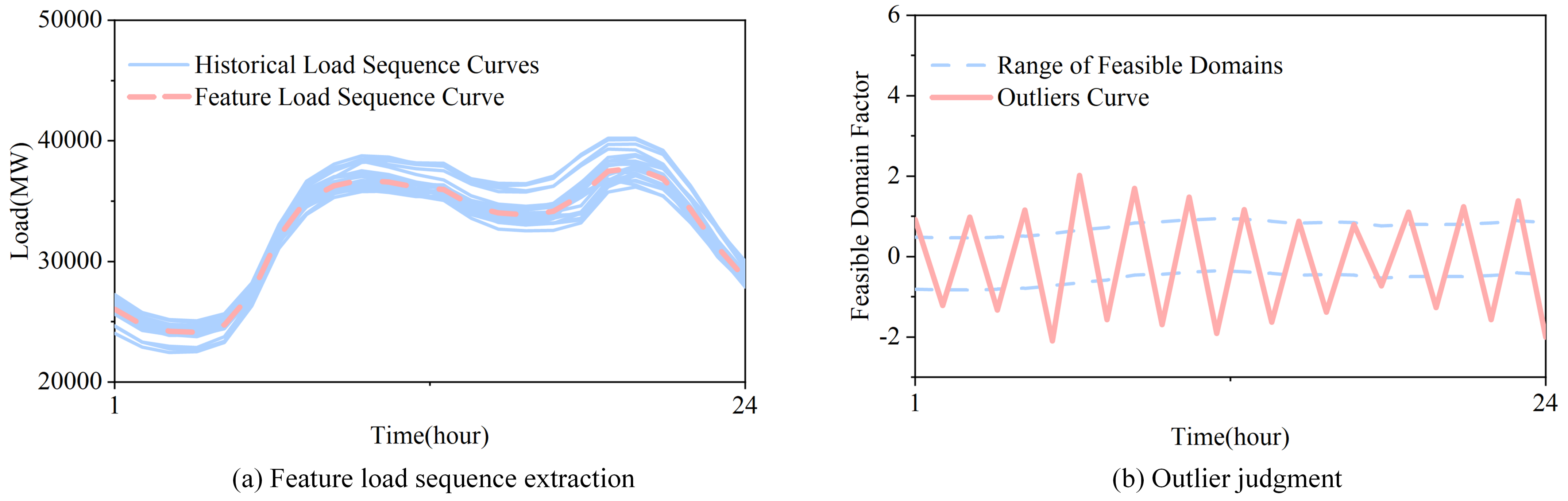
A novel outlier determination method is proposed. In order to cope with inevitable dead numbers and abnormal sensitivity of smart meters and sensors, which lead to missing values and outliers in the transmission process, a data anomaly detection method based on non-parametric Gaussian kernel density estimation is proposed. Using the historical load data to construct the feature curve of customers’ electricity-consumption behavior, the upper and lower limits of the feasible domain are set to determine the anomaly.

(2)

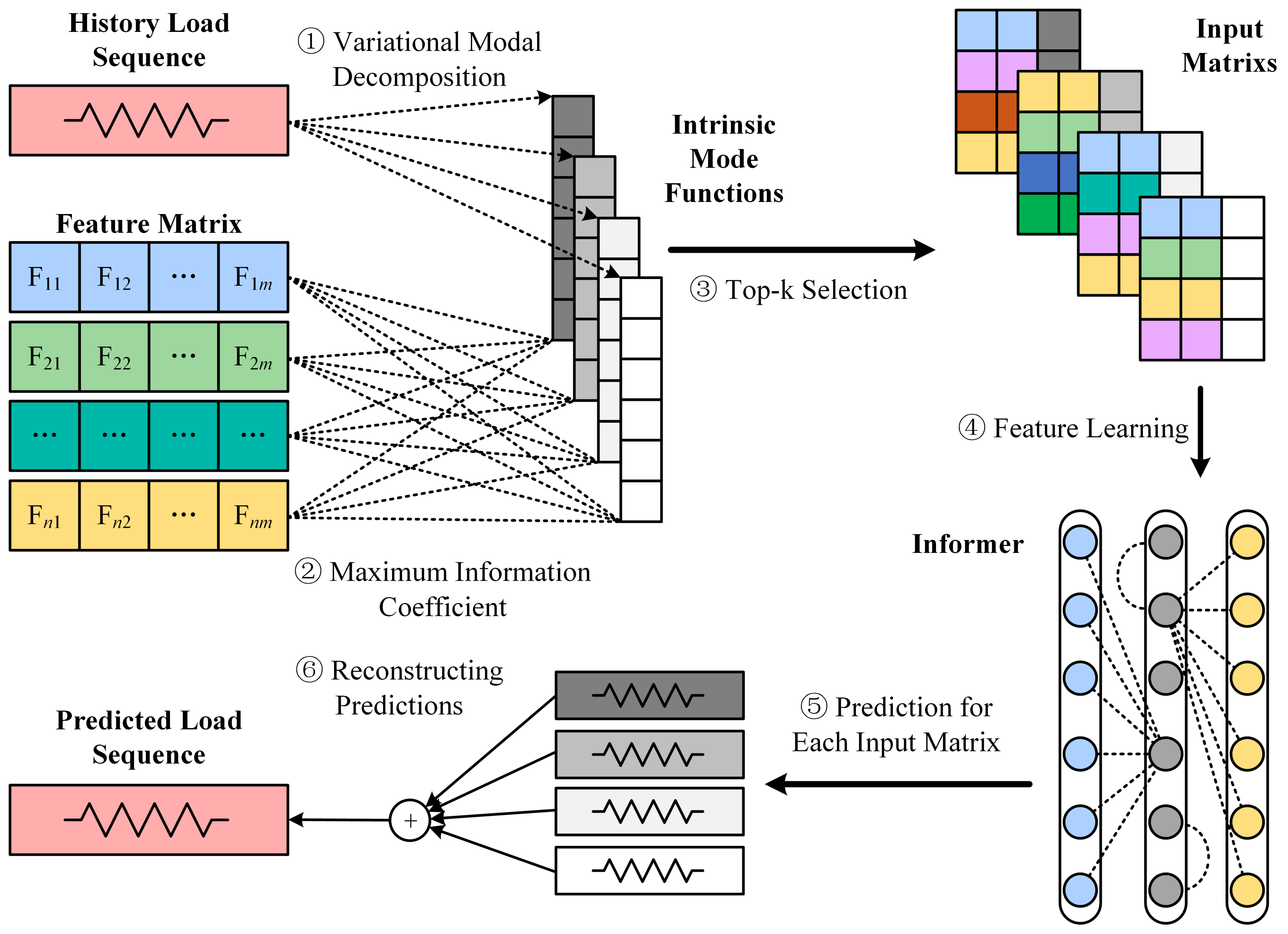
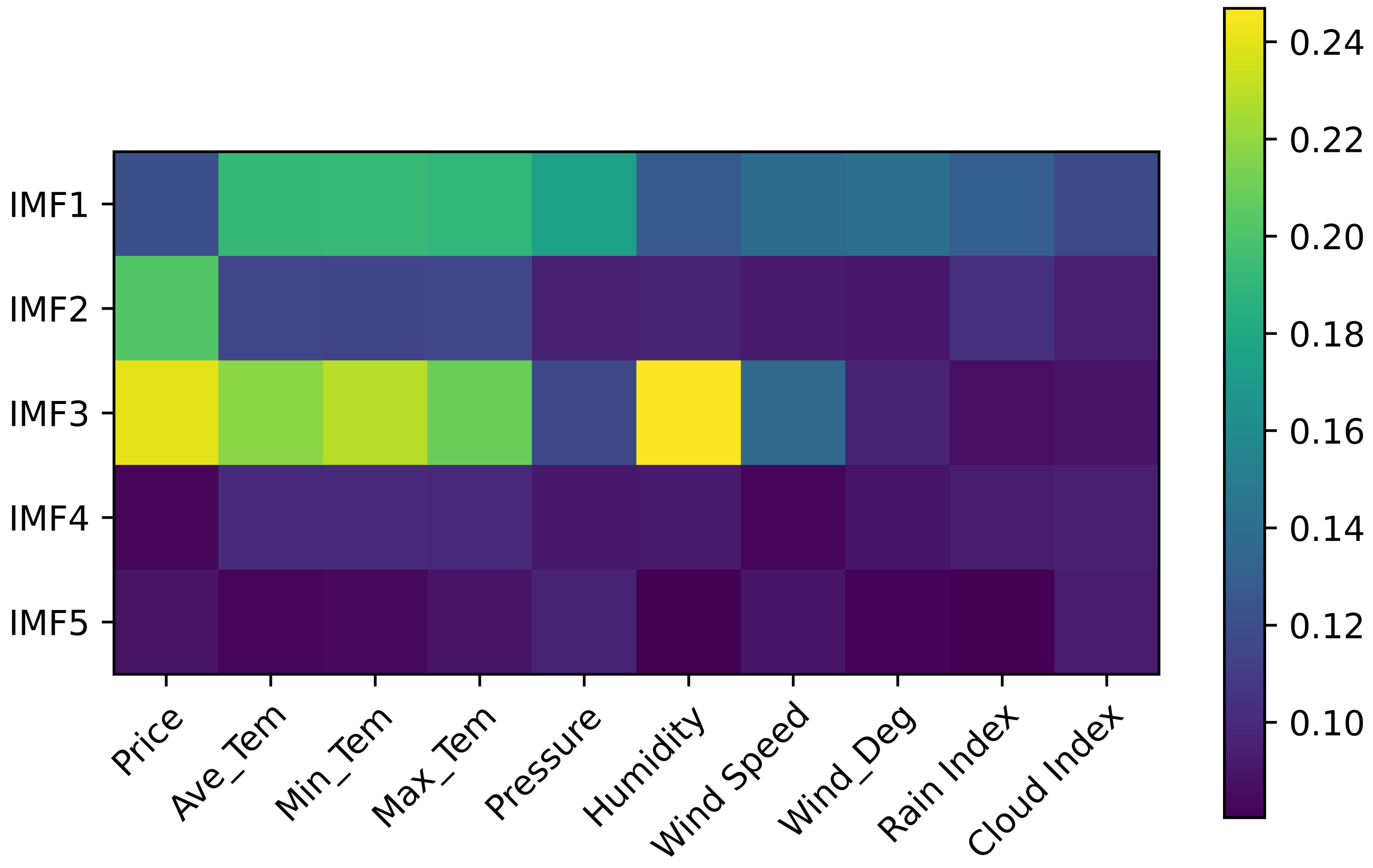
A relatively novel feature-selection method is proposed. The original load signal is decomposed into several IMFs components by VMD. The maximal information coefficient (MIC) is used to find out the non-linear correlation between each IMF and the features, which contain meteorological, geographical, policy and other factors.

(3)

Abandoning the traditional recurrent neural network structure, this paper uses a novel improved self-attention Informer-based model to predict and reconstruct an IMF input matrix. The model is optimized using AdaBelief, which improves the accuracy and operational efficiency of the model operation.

(4)

The strengths and weaknesses of the model are analyzed in depth by comparing other single models with hybrid models and combining several statistical parameters’ evaluation indexes. The accuracy of the model was verified by cross-sectional and longitudinal experiments on a regional-level load dataset in Spain.

The rest of the paper is organized as follows. Section 2 presents the dataset set used in this paper. Section 3 describes the basic steps of STLF. Section 4 gives the specific operations and parameter settings of the experiments, which are compared with other single or combined models to verify the superiority of the model in cross-sectional experiments and longitudinal experiments. Finally, we discuss the conclusions and future work of this paper in Section 5.

2. Data Preparation

The Spanish regional level dataset [22] used in this paper contains three parts: historical load data, meteorological data and electricity price data.

Historical load data are obtained from public electricity consumption data collected by the Spanish Transmission Service Operator, which records the electricity load consumption from 1 January 2015 to 31 December 2018, with a collection frequency of 1 H. The weather data is sourced from Kaggle open source data, obtained from the Open Weather API of five major Spanish cities. The geographical location of these five Spanish cities is shown in Figure A1 in Appendix A.

(1)

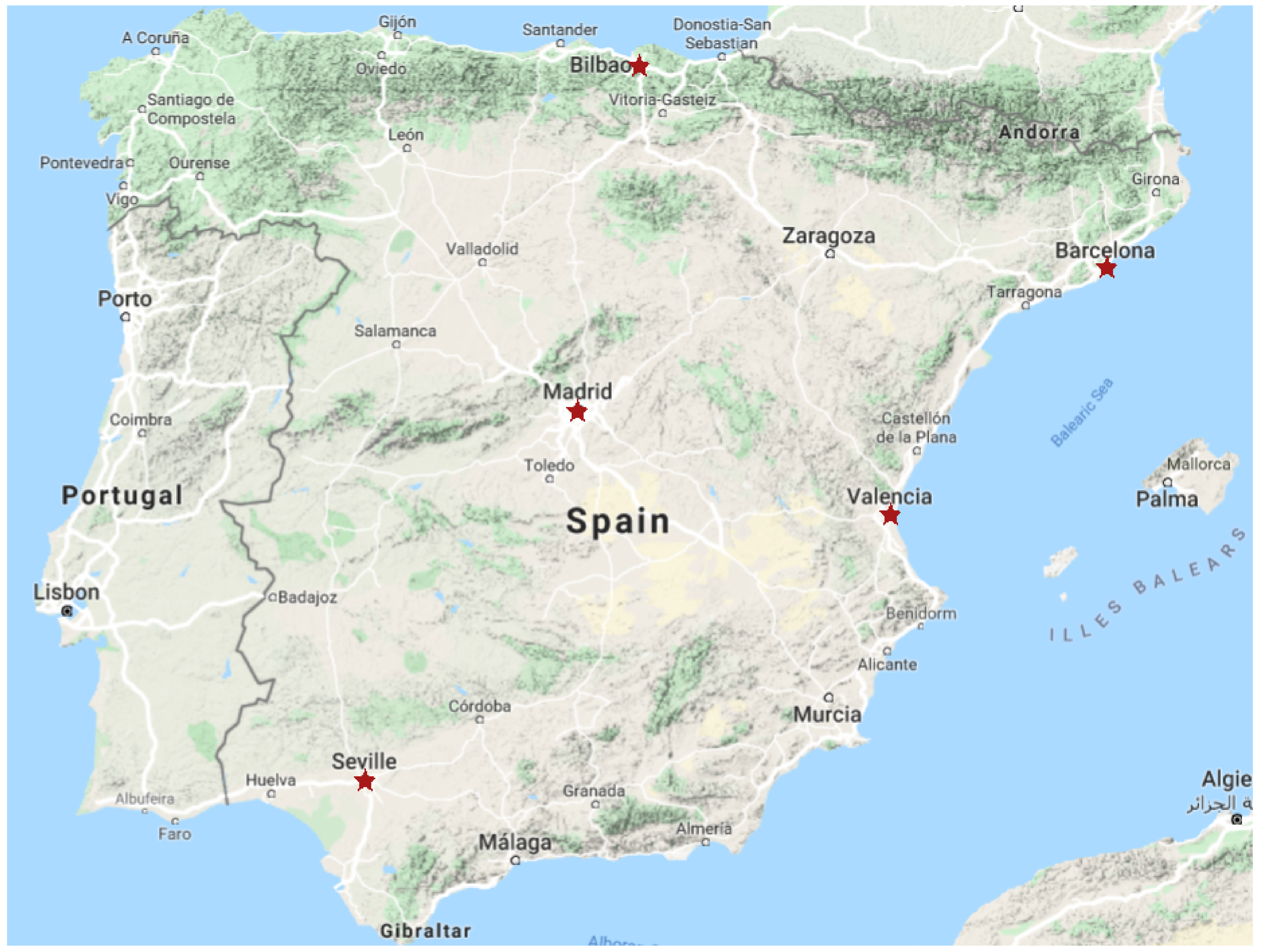
Meteorological data include mean temperature, maximum temperature, minimum temperature, barometric pressure, humidity, wind speed, wind degree, cloud index and rain index.

(2)

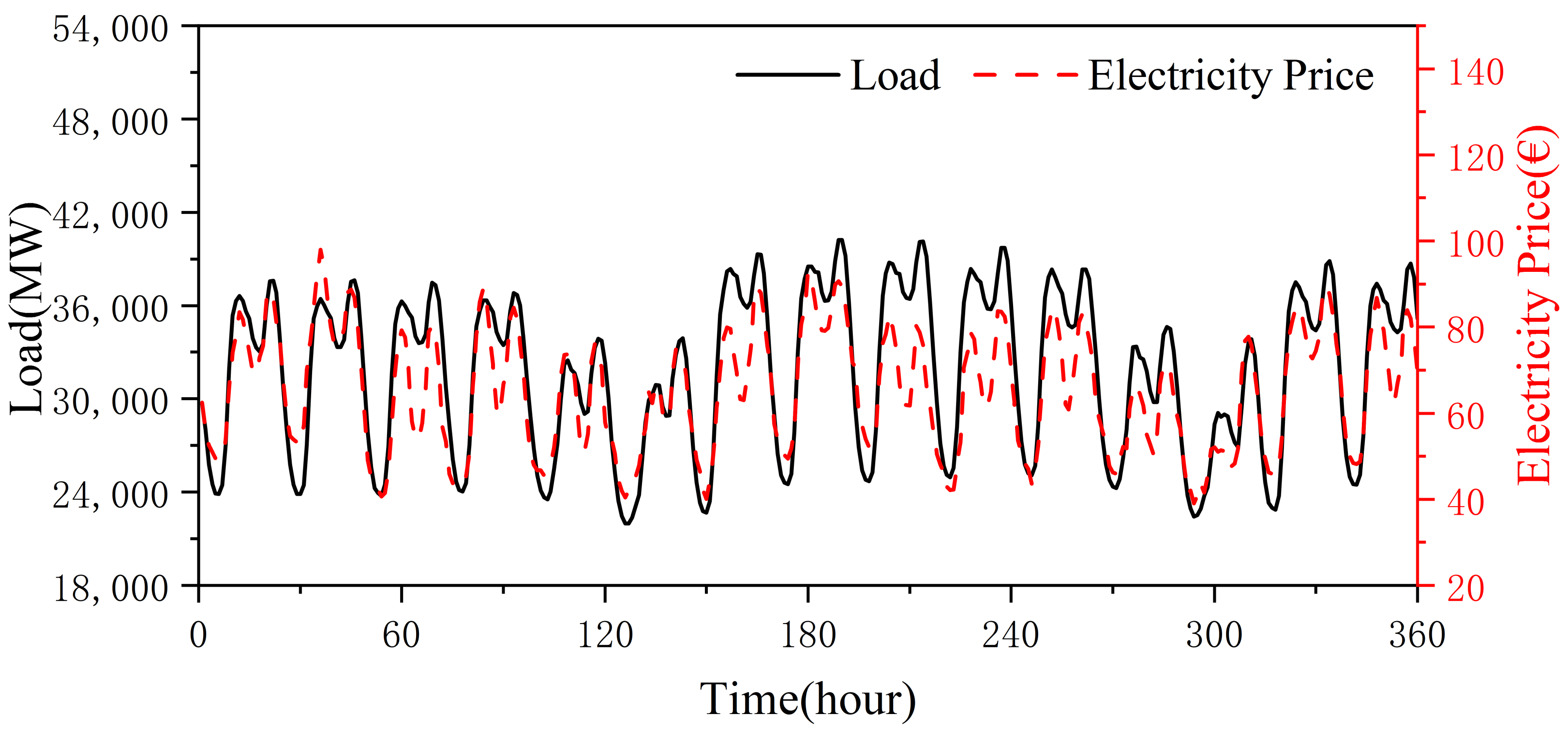
DSM data. Electricity price and load belong to mutual causality, and it can be intuitively seen from Figure 2 that there is a certain correlation between electricity price and load, so electricity price is selected as DSM data.

(3)

The historical load data were divided into a training set, a validation set and a test set in the ratio of 8:1:1. The specific dataset division is shown in

Table 1. Datasets division.

Dataset	Count	Max (MW)	Min (MW)	Mean (MW)	Median (MW)	Std (MW)
Overall	35,064	41,015	18,041	28,697.99	28,902.5	4576.07
Training	28,052	41,015	18,041	28,657.25	28,876.5	4589.24
Validation	3506	40,693	19,706	28,813.13	28,971	4447.79
Test	3506	39,780	18,179	28908.79	29,031	4588.56

.

3. STLF Model

The STLF model uses a dataset from a historical database with real-time sensors. The historical data are used for training and validation of the model, and the real-time data are used for real-time prediction. It is worth mentioning that the historical database is used for the training set, validation set and test set of the paper. Data preprocessing is essential due to problems such as loss and outliers in the process of data collection, transmission and standardization. As shown in Figure 3, in addition to missing and outlier processing, data preprocessing also includes operations such as data normalization, non-numerical data encoding, and dimensionality reduction.

Figure 4 illustrates the process of STLF. First, the historical load sequence is decomposed into several IMFs using VMD, each of which has a different frequency and contains different information. Then, the correlation coefficients of each row in the feature matrix with each IMF are calculated using MIC. Based on the prediction requirements, Top-k of these feature vectors are selected to form the input matrix. After that, the input matrix is brought into Informer to predict separately, and several predictions are obtained. Finally, the predicted values of all input matrices are reconstructed to obtain the final predicted load sequence.

3.1. Outlier Processing

In general, outlier detection is difficult because the threshold value is hard to set. When the threshold value is set too high, it is easy to miss detection; when the threshold value is set too low, it is easy to misjudge. Therefore, for data preprocessing, we propose an anomaly detection method based on non-parametric probability density estimation.

The non-parametric kernel density estimation does not require empirical assumptions about the prior distribution of the data, and is therefore very suitable for constructing customer electricity consumption feature curves. Using the feature curve, the upper and lower limits of the feasible domain can be set to determine the outliers.

3.1.1. Feature Curves Construction

For the target to be detected, we need to obtain its historical load data. Assume the 24 h electricity consumption of a customer on the i-th day is:

$${\mathit{X}}_{\mathit{i}}={\left({\mathit{x}}_{i1},{\mathit{x}}_{i2},\cdots ,{\mathit{x}}_{i24}\right)}^{\mathrm{T}}$$

(1)

The commonly used Gaussian kernel function is chosen as the kernel function for non-parametric kernel density estimation:

$$K\left(x\right)=\frac{1}{\sqrt{2\pi }}{e}^{-\frac{x^2}{2}}$$

(2)

Calculate the probability density function corresponding to the load $x_k$ at the k-th moment of the user’s historical load data:

$$f_k\left(x_k\right)=\frac{1}{Th}\sum _{i=1}^{T}K\left(\frac{x_k-x_{ik}}{h}\right)$$

(3)

where T is the total number of samples and h is the window width.

Calculate the probability density function corresponding to each moment of the user, and form the maximum probability density vector curve for 24 h:

$${\mathit{X}}_{mp}={\left[x_{mp1},x_{mp2},\cdots ,x_{mp24}\right]}^{\mathrm{T}}$$

(4)

Calculate the weights of the i-th day:

$$w_i=\frac{{\left(1/d_i\right)}^{\lambda }}{{\sum }_{i=1}^T{\left(1/d_i\right)}^{\lambda }}$$

(5)

$$d_i=\sqrt{\sum _{n=1}^{24}{\left|x_{ik}-x_{mpn}\right|}^2}$$

(6)

where $\lambda$ is an empirically adjustable parameter, $\lambda \in$ [0,1].

By weighted superposition, the customer electricity consumption feature curve can be obtained as:

$${\mathit{X}}_{fc}=\sum _{i=1}^T{w}_i{\mathit{X}}_i$$

(7)

3.1.2. Feasible Domain Construction

Statistics on the maximum and minimum values of the user’s historical load at each moment:

$$\left\{\begin{array}{c}{\mathit{X}}^{max}=\left[x_1^{max},x_2^{max},\cdots ,x_{24}^{max}\right]\hfill \\ {\mathit{X}}^{min}=\left[x_1^{min},x_2^{min},\cdots ,x_{24}^{min}\right]\hfill \end{array}\right.$$

(8)

The upper and lower limits of the feasible domain are:

$$\left\{\begin{array}{c}{P}^{up}=\frac{K(X^{max}-X_{fc})}{X^{max}-X^{min}}\hfill \\ P^{down}=\frac{K(X^{min}-X_{fc})}{X^{max}-X^{min}}\hfill \end{array}\right.$$

(9)

where K is an empirically adjustable parameter.

For data to be detected $X_d$, its curve on the feasible domain is:

$$P=\frac{K(X_d-X_{fc})}{X^{max}-X^{min}}$$

(10)

when P is within the upper and lower limits of the feasible domain $[P^{down},P^{up}]$, the data to be detected are considered normal. When the limit is crossed, the outlier can be identified.

3.2. Feature Selection

3.2.1. VMD

Regional-level power loads contain cyclical, non-cyclical periodic and trend information. The information hidden in the load series is difficult to strip out from the naked eye only, which results in data with low interpretability. In order to more intuitively understand the physical meaning contained in each component, we need to decompose the electrical load. Variational Modal Decomposition [23] is a signal decomposition estimation method. The main idea is to decompose the raw signal into several smooth IMFs with different frequencies. VMD determines the frequency center and bandwidth of each IMF by iteratively searching for the optimal solution of the variational model, thus adaptively realizing the frequency domain dissection of the signal and the IMF.

The objective of VMD is to minimize the bandwidth sum of all IMFs with the constraint that the sum of all IMFs is equal to the raw signal. The expression is shown as follows:

$$\left\{\begin{array}{c}\underset{\left\{u_k\right\},\left\{{\omega }_k\right\}}{min}\left\{{\sum _k∥{\partial }_t\left[\left(\delta \left(t\right)+\frac{j}{\pi t}\right)\ast u_k\left(t\right)\right]e^{-j\omega t}∥}^2\right\}\hfill \\ s.t.\sum _k{u}_k=f\hfill \end{array}\right.$$

(11)

where $\left\{u_k\right\}=\left\{u_1,\cdots ,u_k\right\}$ denotes the k-th IMFs after VMD.

The quadratic penalty factor $\alpha$ and Lagrange multiplier operator $\lambda \left(t\right)$ are introduced, thus transforming the constrained variational problem into an unconstrained variational problem. The solution is solved by alternately updating $u_k^{n+1}$ and ${\omega }_k^{n+1}$. The pseudo code of VMD is as follows (Algorithm 1).

Algorithm 1 VMD

1:Intialize ${\widehat{u}}_k\leftarrow 0$, ${\omega }_k\leftarrow 0$ 2:Update ${\widehat{u}}_k$ ${{\widehat{u}}_k}^{n+1}\left(\omega \right)=\frac{\widehat{f}\left(\omega \right)-{\displaystyle \sum _{i\ne k}}{\widehat{u}}_i\left(\omega \right)+\frac{1}{2}{\widehat{\lambda }}^n\left(\omega \right)}{1+2\alpha {\left(\omega -{\omega }_k\right)}^2}$ 3:Update ${\omega }_k$ ${{\omega }_k}^{n+1}=\frac{\underset{0}{\overset{\infty }{\int }}\omega {\left|{\widehat{u}}_k\left(\omega \right)\right|}^{2}d\omega }{\underset{0}{\overset{\infty }{\int }}{\left|{\widehat{u}}_k\left(\omega \right)\right|}^{2}d\omega }$ 4:Update ${\widehat{\lambda }}^{n+1}\leftarrow {\widehat{\lambda }}^n+\zeta \left(\widehat{f}-{\sum }_k{\widehat{v}}_k^{n+1}\right)$ until convergence ${\sum }_k{∥{\widehat{v}}_k^{n+1}-{\widehat{v}}_k^n∥}_2^2<ϵ.$

Where ${{\widehat{u}}_k}^{n+1}\left(\omega \right)$ is the Wiener filter of $\widehat{f}\left(\omega \right)-{\displaystyle \sum _{i\ne k}}{\widehat{u}}_i\left(\omega \right)$. ${{\omega }_k}^{n+1}$ is the mode function power spectrum center of gravity. $ϵ$ is the decomposition error.

3.2.2. MIC

The maximal information coefficient is used to measure the degree of data association between two variables, which includes linearity and non-linearity [24].

Assume that X and Y are two random variables in the datasets, where $X=\left\{x_1,\cdots ,x_n\right\}$ and $Y=\left\{y_1,\cdots ,y_n\right\}$, and n is the number of samples. Define the mutual information between X and Y as:

$$I\left(x;y\right)=\int p\left(x,y\right){log}_2\frac{p\left(x,y\right)}{p\left(x\right)p\left(y\right)}dxdy$$

(12)

where $p\left(x,y\right)$ is the joint density function between X and Y. $p\left(x\right)$ and $p\left(y\right)$ denote the marginal probability densities of X and Y, respectively.

Grids are drawn on the data scatter-plot consisting of variables X and Y, and the magnitude of the mutual information between each grid is calculated. The maximum value of mutual information is selected using different grid division criteria and calculated as:

$$MIC\left(x;y\right)=\underset{a\ast b<B}{max}\frac{I\left(x;y\right)}{log{}_{2}min\left(a,b\right)}$$

(13)

where a and b denote the number of meshes divided in the X and Y directions, respectively, and B is the maximum value of the mesh.

3.3. Model Training

3.3.1. Informer

To address the following three problems of the traditional Transformer: (i) the self-attention mechanism leads to the squared computational complexity of the model; (ii) the high memory occupation rate; (iii) the step by step decoding process leads to slow prediction speed and accumulated errors; and the Informer model makes three improvements: (i) the ProSparse self-attention mechanism, which effectively reduces the computational complexity; (ii) self-attention distilling is proposed to reduce the number of dimensions and network parameters; and (iii) a generative-style decoder is proposed to improve the prediction speed. The structure of the Informer is shown in Figure 5.

The traditional self-attention mechanism is mainly composed of Query, Key and Value. The expressions are:

$$A\left(Q,K,V\right)=Softmax\left(\frac{Q{K}^T}{\sqrt{d}}\right)V$$

(14)

where, $Q\in R^{L_Q\times d}$,$K\in R^{L_k\times d}$,$V\in R^{L_V\times d}$, d is the input dimension.

Define the smoothed probability of the ith attention coefficient in the form of:

$$A\left(q_i,K,V\right)={\displaystyle \sum _j}\frac{k\left(q_i,k_i\right)}{{\displaystyle \sum _l}k\left(q_i,k_l\right)}{v}_j=E_{p\left(\left.k_i\right|q_i\right)}\left[V_j\right]$$

(15)

where, $p\left(\left.k_i\right|q_i\right)=\frac{k\left(q_i,k_i\right)}{{\displaystyle \sum _l}k\left(q_i,k_l\right)}$, $k\left(q_i,k_i\right)=exp\left(\frac{q_i{k_j}^T}{\sqrt{d}}\right)$

By visualizing the dot product results in the self-attention mechanism, Zhou et al., found that the long-tail distribution, i.e., the dot product of Query and Key, dominates the overall distribution. Therefore, the computational complexity of the model can be effectively reduced by using the “sparsity” of the self-attention coefficient matrix to filter out the dot products with higher contributions. To measure this matrix “sparsity”, Zhou et al., used the Kullback–Leibler scatter and defined the sparsity evaluation formula for the i-th Query as:

$$M\left(q_i,K\right)=ln\sum _{j=1}^{K_K}{e}^{\frac{q_i{k_j}^T}{\sqrt{d}}}-\frac{1}{L_K}\sum _{j=1}^{L_K}\frac{q_i{K_j}^T}{\sqrt{d}}$$

(16)

where, $ln{\displaystyle \sum _{j=1}^{K_K}}{e}^{\frac{q_i{k_j}^T}{\sqrt{d}}}$ is the logsumexp of $q_i$ on all Keys, $\frac{1}{L_K}{\displaystyle \sum _{j=1}^{L_K}}\frac{q_i{K_j}^T}{\sqrt{d}}$ is the arithmetic mean. By setting upper and lower bounds on $M\left(q_i,K\right)$, Zhou et al. approximated it as:

$$\widehat{M}\left(q_i,K\right)=\underset{j}{max}\left\{\frac{q_i{k_j}^T}{\sqrt{d}}\right\}-\frac{1}{L_K}\sum _{j=1}^{L_K}\frac{q_i{K_j}^T}{\sqrt{d}}$$

(17)

Based on the above theory, Zhou et al. will propose a new self-attention mechanism, ProbSparse self-attention, with the expression:

$$A\left(Q,K,V\right)=Softmax\left(\frac{\widehat{Q}{K}^T}{\sqrt{d}}\right)V$$

(18)

where $\widehat{Q}$ has the same size as Q but contains only $\widehat{M}\left(q_i,K\right)$ under the sparse evaluation $q_i$. That is, the computational complexity is reduced to from $O\left(L^2\right)$ to $O\left(LlnL\right)$.

In the encoder part, since there is a redundant combination of values V in the feature mapping of Encoder, increasing the weights of the dominant features can effectively reduce the data dimensionality. The expression for the distillation operation from layer j to layer $j+1$ is:

$$X_{j+1}^t=MaxPool\left(ELU\left(Convld\left({\left[X_j^t\right]}_{AB}\right)\right)\right)$$

(19)

where ${\left[X_j^t\right]}_{AB}$ contains the multi-head ProbSparse self-attention operation. $Convld$ denotes the one-dimensional convolution operation, $ELU$ is the activation function, and $MaxPool$ is the maximum pooling operation.

The self-attention matrix, after the distillation mechanism, reduces the input sequence length by half in each layer of the decoder, which effectively saves memory overhead and computation time.

In the decoder part, Zhou et al. divide the input sequence into two parts: (i) a known sequence before the time point to be predicted, and (ii) a placeholder sequence of the sequence to be treated, with the expression:

$$X_{feed\_de}^t=Concat\left(X_{token}^t,X_o^t\right)\in R^{\left(L_{token}+L_y\right)\times d_{model}}$$

(20)

In addition to the time series, Zhou et al. also use the position vector and temporal information as inputs. Moreover, to avoid the model self-regressing during the prediction process, a masked multi-head attention mechanism is used, which hides the information after the current predicted position. This generative-style decoder allows the model to generate the entire prediction sequence at once, which greatly reduces the prediction decoding time.

3.3.2. AdaBelief

Based on the classic optimizer Adam [25], AdaBelief [26] adjust the training stride according to the Belief in the gradient direction. The pseudo-code for both is as follows (Algorithms 2 and 3).

Algorithm 2 Adam

1:Intialize ${\theta }_0$, $M_0\leftarrow 0$, $v_0\leftarrow 0$, $t\leftarrow 0$ 2:While $\theta$ is not converged: $t\leftarrow t+1$, $g_t\leftarrow {\nabla }_{\theta }{f}_t\left({\theta }_{t-1}\right)$, $M_t\leftarrow {\beta }_1{M}_{t-1}+(1-{\beta }_1)g_t$, $v_t\leftarrow {\beta }_2{s}_{t-1}+(1-{\beta }_2){g_t}^2$ 3:Update ${\theta }_t\leftarrow \prod {}_{\mathcal{F},\sqrt{v_t}}\left({\theta }_{t-1}-\alpha \frac{M_t}{\sqrt{v_t+\epsilon }}\right)$

Algorithm 3 AdaBelief

1:Intialize ${\theta }_0$, $M_0\leftarrow 0$, $s_0\leftarrow 0$, $t\leftarrow 0$ 2:While $\theta$ is not converged: $t\leftarrow t+1$, $g_t\leftarrow {\nabla }_{\theta }{f}_t\left({\theta }_{t-1}\right)$, $M_t\leftarrow {\beta }_1{M}_{t-1}+(1-{\beta }_1)g_t$, $s_t\leftarrow {\beta }_2{s}_{t-1}+(1-{\beta }_2){(g_t-M_t)}^2$ 3:Update ${\theta }_t\leftarrow \prod {}_{\mathcal{F},\sqrt{s_t}}\left({\theta }_{t-1}-\alpha \frac{M_t}{\sqrt{s_t+\epsilon }}\right)$

Where $g_t$ represents the t-th step, $M_t$ represents the exponential moving average (EMA) of $g_t$, and $\alpha$ is learning rate. AdaBelief replaces $v_t$ in Adam with $s_t$. $v_t$ and $s_t$ are EMA of ${g_t}^2$ and ${(g_t-M_t)}^2$, respectively.

4. Simulation Environment and Experimental Results

4.1. Experimental Environment and Evaluation Metrics

All experiments in this paper were run in a Python 3.8 environment with deep learning models using Pytorch and Tensorflow libraries. The experimental hardware CPU utilizes an Intel Core i5-9300H processor, the GPU utilizes an NVIDIA GeForce RTX 2060 graphics card and the memory is 16 GB.

To measure the prediction accuracy, this paper uses mean absolute percentage error (MAPE) and root mean square error (RMSE). For the predicted value y, the true value $\overline{y}$, the formula is as follows:

$$MAPE=\frac{100\%}{n}\sum _{i=1}^n\left|\frac{\overline{y_i}-y_i}{y_i}\right|$$

(21)

$$RMSE=\sqrt{\frac{1}{n}{\displaystyle \sum _{i=1}^n}{\left(\overline{y_i}-y_i\right)}^2}$$

(22)

We chose a model with a sliding window width of 96 and a step length of 1 for prediction. That is, the data of the first 96 h were used to make predictions for the next moment, thus guaranteeing that the prediction model had sufficient data for learning. The prediction process is shown in Figure 6.

4.2. Experimental Results

4.2.1. Experiment I: Outlier Detection

A sample of 21 working days of electricity from late January to early February in the Spanish electricity consumer dataset was selected for the arithmetic analysis. The data granularity is 1 h, and there are 24 × 21 = 504 data in this sample. The electricity consumption of the 21 working days is superimposed and the feature load sequence are extracted using the method of this paper. The results are shown in Figure 7a.

To verify the feasibility of the method, the datasets with outliers were generated.The electricity consumption data for a randomly selected day was scaled up by ten percent for odd time-points and scaled down by ten percent for even time-points.The experimental results are shown in Figure 7b.

The scaled data points exceeded the upper and lower limits of the feasible domain and were identified as anomalous data points. This demonstrates that the proposed method, although simple, can effectively detect outliers. In fact, the inspector can adjust the parameter K in order to adjust the model detection tightness according to the requirements.

4.2.2. Experiment II: STLF Cross-Sectional Experiment

The original signal was decomposed using VMD. After repeated experiments, the center frequency was closest when the number of IMF decomposition K was greater than 5, so K was taken as 5; penalty factor = 2700; center limit frequency = 0. The original power load and each IMF after decomposition are shown in Figure 8.

The modal function IMF1 never crossed zero and contained the trend direction of the original load. The modal functions IMF2 and IMF3 had a lower and more regular over-zero rate and contain more periodic information. The modal functions IMF4 and IMF5 had higher and less regular over-zero rates and contained more non-periodic information. In order to better describe the information contained in the IMFs after VMD decomposition, MIC was used to select the features to enhance the prediction ability and reduce the information loss due to VMD decomposition. Figure 9 visualizes the heat map of the MIC coefficient matrix. The impact features vary for each IMF. We selected the three to six features with the highest relevance to build the input matrix. In this experiment, a total of five input matrices were obtained.

Bringing all the input matrices into Informer for prediction separately and reconstructing all the predictions, we obtained the final predicted values. The predicted results and the actual load are shown in Figure 10. It can be seen that the two fit well, which implies that the proposed model has some significance for short-term-load forecasting studies.

In order to show the superiority of the proposed models more objectively, some classical machine learning algorithms were used to perform comparative experiments. These models and their optimal parameters are shown in

Table A3. Models and Parameters.

Models	Parameters
Proposed	The learning rate is 0.01, the input sequence length is 96, the prediction sequence length is 1, the number of head is 8, the number of encoder is 2, the number of decoder is 1, the dropout rate is 0.05, the activation function is “GELU”.
XGBoost	The learning rate is 0.01, the max depth of trees is 6, iteration is 100, colsample is 0.95, alpha is 0.1, lambda is 0.15, gamma is 0.1, min child weight is 0.1.
CNN	The learning rate is 0.001, the nunber of convolution layers is 1, the number of filters in convolution layer is 48, the kernel size is 2, the strides is 1, the number of fully connected layers is 2, the number of neurons in fully connected layers is set 48/1,the activation function is “ReLU”.
TCN	The learning rate is 0.001, the nunber of convolution layers is 1, the number of filters in convolution layer is 64, the kernel size is 2, the strides is 1, the dilations are (1,2,4,8,16,32), the dropout rate is 0.2, the number of fully connected layers is 2, the number of neurons in fully connected layers is set 64/1,the activation function is “ReLU”.
GRU	The learning rate is 0.001, the number of hidden layers is 1, the number of nodes in hidden layer is 128, the dropout rate is 0.1, the number of fully connected layers is 2, the number of neurons in fully connected layers is set 128/1, the activation function is “tanh”.
LSTM	The learning rate is 0.001, the number of hidden layers is 1, the number of nodes in hidden layer is 128, the dropout rate is 0.1, the number of fully connected layers is 2, the number of neurons in fully connected layers is set 128/1, the activation function is “tanh”.
MLP	The learning rate is 0.001, the number of hidden layers is 4, the number of nodes in hidden layer are (256,128,64,32), the dropout rate is 0.2, the number of fully connected layers is 2, the number of neurons in fully connected layers is set 32/1, the activation function is “ReLU”.
SVR	The kernel is “rbf”, all other parameters are default parameters.

in the Appendix A. The experimental results are shown in Figure 11.

MLP, SVR and XGBoost had the worst prediction performance, achieving the highest prediction error among the traditional machine learning models. This is due to the inability of traditional machine-learning algorithms to effectively extract the high-dimensional features of the data in a complex predictive environment. The prediction performance of CNN and TCN was slightly better than traditional machine-learning algorithms. lSTM and GRU achieved good results, reducing the prediction error to within two percent. The proposed model had the best prediction performance with MAPE below one percent

Compared to the single model, it is clear from the results that the hybrid model generally outperformed the single model in terms of prediction performance and the feature extraction effect of TCN was better than CNN.

In order to verify the robustness of the proposed model, we selected a larger-scale prediction step length for the experiment. As can be seen from Figure 11, the prediction error increased for almost all models as the prediction step length increased. This is due to the cumulative effect of the error, i.e., the prediction of the load at the second moment was substituted for the predicted value at the first moment. In fact, this error accumulation is unavoidable. Compared with other models, the proposed model did not show much error growth in this process, and thus has some robustness.

4.2.3. Experiment III: STLF Longitudinal Experiments

To verify that the proposed VMD-MIC feature-selecting method is effective, we also conducted longitudinal experiments, also known as ablation experiments.

The so-called ablation experiment is to remove a module of the proposed model to test its predictive performance. To make the results more objective, we need to ensure that the model is identical to the parameters. The four ablation models are as follows.

(1)

The proposed model.

(2)

VMD-Informer. The load was decomposed using VMD according to the same parameters as in the cross-sectional experiment. The MIC correlation analysis module was abandoned and all features were entered in the construction of the input matrix for prediction.

(3)

MIC-Informer. Correlation analysis was performed using MIC for loads only, and Top-k features were selected for detection.

(4)

Simple Informer. We dissolved all the modules and kept only the original Informer for load forecasting. We retained all features in the prediction.

The results of the ablation experiment are shown in Figure 11. The experimental results show that the prediction accuracy of the above two models is between the proposed model and the plain Informer model, i.e., the VMD-MIC feature selection method is helpful to improve the load prediction accuracy. Among them, VMD reduced the error by 0.43% and MIC only reduced the error by less than 0.1.

As the prediction step length increased, the prediction error of all models gradually increased. However, the proposed model achieved the best prediction accuracy in all step length; this means that it also had the best robustness compared to the ablation model.

4.2.4. Experiment IV: AdaBelief Optimization Experiment

Finally, this paper presents a comparative experiment on the optimization performance of Adabelief. The commonly used SGD [27] and Adam optimizers were selected as benchmarks. Under the same experimental environment, the prediction accuracy and convergence speed are shown in

Table 2. Results of optimizer comparison experiments.

Optimizer	MAPE (%)	RMSE (MW)	Convergence Epoch
AdaBelief	0.98	330.89	12
Adam	2.56	969.05	3
SGD	1.39	478.68	18

.

As can be seen from Table 2, although AdaBelief achieved the best prediction accuracy, it did not have the best convergence rate. As the most classical optimizer, Adam achieved the best results in terms of convergence speed and had an SGD in between.

5. Conclusions

In this paper, a self-attention-based short-term load forecasting considering demand-side management was proposed. From the example study, the following conclusions can be drawn.

(1)

The method uses a non-parametric Gaussian kernel density estimate to fit the user load feature curve. Outliers are identified by setting upper and lower limits on the feasible domain for the load.

(2)

The VMD-MIC feature filtering method optimizes the input feature dimension. After ablation experiments, it is proved that the prediction accuracy of the combined model is higher than that of the ablated single model.

(3)

Cross-sectional and longitudinal experiments are conducted on a regional-level load dataset set in Spain. The experimental results prove that the proposed method is superior to other methods.

(4)

Optimizing the proposed model using AdaBelief can significantly improve the prediction accuracy, but will reduce the convergence speed.

(5)

With the development of DSM, our work will focus on the study of more types and scales of customer electricity-consumption data.

References

1. Kong, X.; Li, C.; Zheng, F.; Wang, C. Improved deep belief network for short-term load forecasting considering demand-side management. IEEE Trans. Power Syst. 2019, 35, 1531–1538. [Google Scholar] [CrossRef]
2. Wang, H.; Ruan, J.; Wang, G.; Zhou, B.; Liu, Y.; Fu, X.; Peng, J. Deep learning-based interval state estimation of AC smart grids against sparse cyber attacks. IEEE Trans. Ind. Inform. 2018, 14, 4766–4778. [Google Scholar] [CrossRef]
3. Arora, S.; Taylor, J.W. Short-term forecasting of anomalous load using rule-based triple seasonal methods. IEEE Trans. Power Syst. 2013, 28, 3235–3242. [Google Scholar] [CrossRef] [Green Version]
4. Massaoudi, M.; Refaat, S.; Abu-Rub, H.; Chihi, I.; Oueslati, F.S. PLS-CNN-BiLSTM: An end-to-end algorithm-based Savitzky–Golay smoothing and evolution strategy for load forecasting. Energies 2020, 13, 5464. [Google Scholar] [CrossRef]
5. Alonso, A.M.; Nogales, F.J.; Ruiz, C. A single scalable LSTM model for short-term forecasting of massive electricity time series. Energies 2020, 13, 5328. [Google Scholar] [CrossRef]
6. Wang, Y.; Chen, Q.; Zhang, N.; Wang, Y. Conditional residual modeling for probabilistic load forecasting. IEEE Trans. Power Syst. 2018, 33, 7327–7330. [Google Scholar] [CrossRef]
7. Browell, J.; Fasiolo, M. Probabilistic Forecasting of Regional Net-load with Conditional Extremes and Gridded NWP. IEEE Trans. Smart Grid 2021, 12, 5011–5019. [Google Scholar] [CrossRef]
8. Kong, W.; Dong, Z.Y.; Hill, D.J.; Luo, F.; Xu, Y. Short-term residential load forecasting based on resident behaviour learning. IEEE Trans. Power Syst. 2017, 33, 1087–1088. [Google Scholar] [CrossRef]
9. Xie, J.; Hong, T. Variable selection methods for probabilistic load forecasting: Empirical evidence from seven states of the united states. IEEE Trans. Smart Grid 2017, 9, 6039–6046. [Google Scholar] [CrossRef]
10. Kong, W.; Dong, Z.Y.; Jia, Y.; Hill, D.J.; Xu, Y.; Zhang, Y. Short-Term Residential Load Forecasting Based on LSTM Recurrent Neural Network. IEEE Trans. Smart Grid 2017, 10, 841–851. [Google Scholar] [CrossRef]
11. Wang, Y.; Chen, J.; Chen, X.; Zeng, X.; Kong, Y.; Sun, S.; Guo, Y.; Liu, Y. Short-term load forecasting for industrial customers based on TCN-LightGBM. IEEE Trans. Power Syst. 2020, 36, 1984–1997. [Google Scholar] [CrossRef]
12. Zhao, B.; Wang, Z.; Ji, W.; Gao, X.; Li, X. A short-term power load forecasting method based on attention mechanism of CNN-GRU. Power Syst. Technol. 2019, 43, 4370–4376. [Google Scholar]
13. Alhussein, M.; Aurangzeb, K.; Haider, S.I. Hybrid CNN-LSTM model for short-term individual household load forecasting. IEEE Access 2020, 8, 180544–180557. [Google Scholar] [CrossRef]
14. Xu, J.H.; Wang, X.W.; Yang, J.J. Short-term Load Density Prediction Based on CNN-QRLightGBM. Power Syst. Technol. 2020, 44, 3409–3416. [Google Scholar]
15. Yao, C.W.; Yang, P.; Liu, Z.J. Load forecasting method based on CNN-GRU hybrid neural network. Power Syst. Technol. 2020, 44, 3416–3424. [Google Scholar]
16. Vaswani, A.; Shazeer, N.; Parmar, N.; Uszkoreit, J.; Jones, L.; Gomez, A.N.; Kaiser, L.; Polosukhin, I. Attention is all you need. Adv. Neural Inf. Process. Syst. 2017, 30, 5998–6008. [Google Scholar]
17. Zhou, H.; Zhang, S.; Peng, J.; Zhang, S.; Li, J.; Xiong, H.; Zhang, W. Informer: Beyond efficient transformer for long sequence time-series forecasting. In Proceedings of the AAAI, Virtual, 2–9 February 2021. [Google Scholar]
18. Fan, C.; Sun, Y.; Zhao, Y.; Song, M.; Wang, J. Deep learning-based feature engineering methods for improved building energy prediction. Appl. Energy 2019, 240, 35–45. [Google Scholar] [CrossRef]
19. Chen, H.; Wang, J.; Tang, B.; Xiao, K.; Li, J. An integrated approach to planetary gearbox fault diagnosis using deep belief networks. Meas. Sci. Technol. 2016, 28, 025010. [Google Scholar] [CrossRef]
20. Lai, G.; Chang, W.C.; Yang, Y.; Liu, H. Modeling long and short-term temporal patterns with deep neural networks. In Proceedings of the 41st International ACM SIGIR Conference on Research and Development in Information Retrieval, Ann Arbor, MI, USA, 8–12 July 2018; pp. 95–104. [Google Scholar]
21. Li, W.; Quan, C.; Wang, X.; Zhang, S. Short-Term Power Load Forecasting Based on a Combination of VMD and ELM. Pol. J. Environ. Stud. 2018, 27, 2143–2154. [Google Scholar] [CrossRef]
22. Shi, H.; Wang, L.; Scherer, R.; Woźniak, M.; Zhang, P.; Wei, W. Short-Term Load Forecasting Based on Adabelief Optimized Temporal Convolutional Network and Gated Recurrent Unit Hybrid Neural Network. IEEE Access 2021, 9, 66965–66981. [Google Scholar] [CrossRef]
23. Dragomiretskiy, K.; Zosso, D. Variational mode decomposition. IEEE Trans. Signal Process. 2014, 62, 531–544. [Google Scholar] [CrossRef]
24. Reshef, D.N.; Reshef, Y.A.; Finucane, H.K.; Grossman, S.R.; Mcvean, G.; Turnbaugh, P.J.; Lander, E.S.; Mitzenmacher, M.; Sabeti, P.C. Detecting novel associations in large data sets. Science 2011, 334, 1518–1524. [Google Scholar] [CrossRef] [PubMed] [Green Version]
25. Kingma, D.; Ba, J. Adam: A Method for Stochastic Optimization. arXiv 2014, arXiv:1412.6980. [Google Scholar]
26. Zhuang, J.; Tang, T.; Ding, Y.; Tatikonda, S.C.; Dvornek, N.; Papademetris, X.; Duncan, J. Adabelief optimizer: Adapting stepsizes by the belief in observed gradients. Adv. Neural Inf. Process. Syst. 2020, 33, 18795–18806. [Google Scholar]
27. Bottou, L. Large-Scale Machine Learning with Stochastic Gradient Descent. In Proceedings of the 19th COMPSTAT, Paris, France, 22–27 August 2010. [Google Scholar]
Figure 1. Power and information flow in DSM.
Energies 15 04198 g001
Figure 2. Price signals motivate DR.
Energies 15 04198 g002
Figure 3. Flow chart of data preprocessing.
Energies 15 04198 g003
Figure 4. Flow chart of STLF model.
Energies 15 04198 g004
Figure 5. Brief structure of Informer.
Energies 15 04198 g005
Figure 6. Sliding window in the prediction process.
Energies 15 04198 g006
Figure 7. Outlier detection experiment results.
Energies 15 04198 g007
Figure 8. VMD results.
Energies 15 04198 g008
Figure 9. MIC correlation analysis.
Energies 15 04198 g009
Figure 10. Prediction results of the proposed model.
Energies 15 04198 g010
Figure 11. Results of the comparison experiment.
Energies 15 04198 g011