Article

Modeling and Simulation of Extended-Range Electric Vehicle with Control Strategy to Assess Fuel Consumption and CO2 Emission for the Expected Driving Range

Faculty of Automotive and Construction Machinery Engineering, Warsaw University of Technology, 02-524 Warsaw, Poland
*
Author to whom correspondence should be addressed.
Energies 2022, 15(12), 4187; https://doi.org/10.3390/en15124187
Submission received: 15 April 2022 / Revised: 30 May 2022 / Accepted: 1 June 2022 / Published: 7 June 2022
(This article belongs to the Special Issue Frontiers in Hybrid Vehicles)

Abstract

:
Extended-Range Electric Vehicles (EREVs) are intended to improve the range of battery electric vehicles and thus eliminate drivers’ concerns about running out of energy before reaching the desired destination. This paper gives an insight into EREV’s performance operating according to the proposed control strategy over various driving cycles, including the Worldwide Harmonized Light-duty Test Cycle Class 3b (WLTC 3b), Federal Test Procedure (FTP-75), and China Light-Duty Vehicle Test Cycle (CLTC-P). Simulation runs were performed in Matlab-Simulink® for different cases of drive range, electricity mix, and vehicle mass. The control strategy goal was to aim at a specified value of battery state of charge at the targeted range value. The obtained test results included: pure electric drive range, acceleration times, EREV range tests, control strategy range errors, Range Extender (REX) utilization metric and distribution of its engagement instances, fuel consumption, total equivalent CO2 emission, powertrain efficiency, and specific energy consumption. The control strategy operated on average with a range error of −1.04% and a range mean square error of 2.13%. Fuel consumption (in range extension mode) varied between 1.37 dm3/100 km (FTP-75) and 6.85 dm3/100 km (WLTC 3b Extra-High 3). CO2eq emission was 95.3–244.2 g/km for Poland, 31.0–160.5 g/km for EU-27, and 1.2–147.6 g/km for Sweden. This paper is a valuable source of information for scientists and engineers seeking to learn the advantages and shortcomings of EREV drives with a proposed control strategy, based on various sets of results.

1. Introduction

The growing awareness of the negative impact of road transport on the environment enforces the introduction of radical changes in vehicles and transport as a whole [1,2]. Fast progress can be observed in the field of vehicle drives [3,4]. It is a consequence of the need to reduce pollutant emissions and fuel consumption—two aspects that cause the greatest concern. One of the effective ways to solve these environmental problems seems to be the use of electric drives [5,6]. However, many technical issues remain to be solved before electric vehicles can compete realistically with conventional vehicles with Internal Combustion Engines (ICEs) [7,8]. A prime example is the relatively small range of an electric vehicle, which is associated with a large mass of battery necessary to store energy in a vehicle, and therefore with high cost [9]. In order to overcome this problem, EREVs were introduced [10].
The general idea of EREV is to use a low displacement combustion engine coupled with an electric generator (REX) as an additional source of electricity, ensuring the recharge of the vehicle’s battery when needed. This allows a significant extension of the vehicle driving range compared to pure electric vehicles, while it is still possible to drive in “zero emission” mode, i.e., by exclusively using electric energy stored in the battery, and recovering part of the energy released during braking [11]. EREV performance depends on many factors, related not only to the construction parameters of the vehicle and the adopted control strategy of the propulsion system, but also to the actual operating conditions of a vehicle and driver behavior [12].
The control strategy, or in other words energy management strategy, of any vehicle that combines two or more energy sources, e.g., petroleum fuel and electricity, determines the path of the power flow between elements of the propulsion system while respecting numerous constraints. Motivations for implementing such strategies vary, but the aim is usually to achieve the lowest energy consumption or pollutant emission. Different strategies have been studied and documented in the literature over the last decade. In general, they can be classified into three categories: rule-based, optimization-based, and a mix of the two [13,14,15,16,17].
The basic idea of the rule-based strategy is that the controller follows predefined rules to process a set of data characterizing the current driving conditions and giving out an output to the elements of the propulsion system [16]. The development of such a strategy requires engineering experience and intuition, as well as mathematical models and experimental results. These kinds of strategies use threshold-based logic with numerous sets of static parameters [16,17,18]. The main advantage of rule-based strategies is their high computational efficiency [13,15,19]. However, the rules are designed and optimized for certain driving conditions (driving cycle). This means that the rules must be recalibrated in the case of a difference between the ‘theoretical’ and the actual driving cycle. Otherwise, the optimal State of Charge (SOC) and the fuel economy of a vehicle may not be reached [13]. Some examples of rule-based methods include: on/off strategy, geometric control, closed-loop control, and fuzzy logic control [16,20].
Optimization-based strategies are applying optimal control theory and one or more optimization methods to a hybrid power system, using mathematical calculations or dynamic functions to minimize vehicle energy consumption or pollutant emissions over a predefined driving cycle [21,22]. Some of the optimization-based strategies, like global optimization control strategies, require prior knowledge of the trip, so usually, they are used off-line, after the fact—to find the optimal solution that could have been implemented. Other optimization-based strategies group called instantaneous optimization control strategies rely on the instantaneous working characteristics of vehicle components, therefore do not need to know all working conditions in advance [23,24]. On the other hand, there are some recent works [21] showing the possibility of real-time operating optimization-based methods through online computing. Researchers use various methods to find the optimum of the considered parameter. The most common include: genetic algorithm [25], dynamic programming [26,27,28], Pontryagin’s minimum principle [19,29,30] and particle swarm optimization [31,32]. It should be noted that optimization-based strategies are computationally intensive and rather complex. Therefore, they may need further research to be viable for implementation in vehicles.
Mixed strategies benefit from the advantages of both approaches: rule-based and optimization-based [24,33]. The general concept of mixed strategy consists of two steps. Firstly, the operating parameters of vehicle propulsion are determined by using optimization methods. Then rule-based algorithms implement these parameters in real-time controllers within the vehicle. In this way, it is possible to overcome the ‘computational barrier’, which makes it difficult to apply online optimization methods in vehicles.
This paper focuses on the application of a specific strategy to control the operation of REX. In this regard, the scientific literature distinguishes between two main approaches: the power demand following strategy and the optimal range strategy [16].
The power following strategy is meant to ensure that REX supplies sufficient power to support the battery in meeting the current power demand of the vehicle. For such a task, the REX operates most of the time providing a great share of power directly to the electric motor. However, the challenge is to ensure the acceptable efficiency of the system, which is limited by the efficiency boundaries of the ICE. Thus, one of the disadvantages of this strategy is low energy conversion by the REX during aggressive and high-duty operations [16]. Selecting the ideal operating curve of an ICE is one of the topics of recent scientific works [34,35,36]. Further optimization is possible through online driving cycle/power predictions for the control strategy. In [37] the ICE followed the total power demand while its output torque remained within a high-fuel-efficiency area. Another study [38] highlighted the possible benefits of control power distributions of REX and battery during the charge sustaining operation mode by using strategies based on dynamic programming and pseudo-spectral optimal control.
The optimal range strategy places priority on keeping the REX at peak fuel efficiency. It requires the ICE to operate only in some fixed optimized points or a certain operating range, e.g., three operation points with high energy efficiency were selected in [39]. At the same time, REX does not always start if the battery SOC is high enough. Finally, the optimal range strategy brings more precise results when it is combined with additional variables, such as motor power demand, battery SOC, current driver driving pattern, and charging efficiency [16,34,40].
The scientific literature on designing REX control strategies and choosing ICE operation points is very rich. In [41] REX efficiency for different ICE operating points was investigated by using real-world driving cycle data. The study [36] introduces a control strategy aimed at extending the battery life and maximizing ICE fuel efficiency by adopting dynamic programming to extract driving pattern data. A similar strategy was applied to an extended range electric bus, as described in [42]. Paper [35] extends the scope of the studied effects to include pollutant emissions from the ICE. In this case, optimal efficiency curves for the REX were obtained with the use of trajectory optimization.
The optimal range strategies can be significantly improved using machine learning and mathematical optimization methods [16]. For instance, promising results were achieved for neural networks utilizing two parameters: battery SOC and distance to the gas stations [43]. A much more complex solution to the same issue was proposed in the paper [44], where stochastic model predictive control is employed to identify the driver’s behavior. As a result, the developed strategy is determined by the driving style and traffic conditions.
This paper shows various component models integrated to make a complete model for simulation of EREV structure. It includes a detailed description of the used control strategy, based on Proportional-Integral (PI) control, tracking battery SOC versus traveled range. The goal was to use the simulation model for a variety of inputs (driving conditions, namely six driving cycles and six constant speeds, three vehicle mass values, and three cases of grid electricity mix) to produce insightful simulation results on Battery Electric Vehicle (BEV) mode operation and EREV operation with a proposed REX control strategy. These results are:
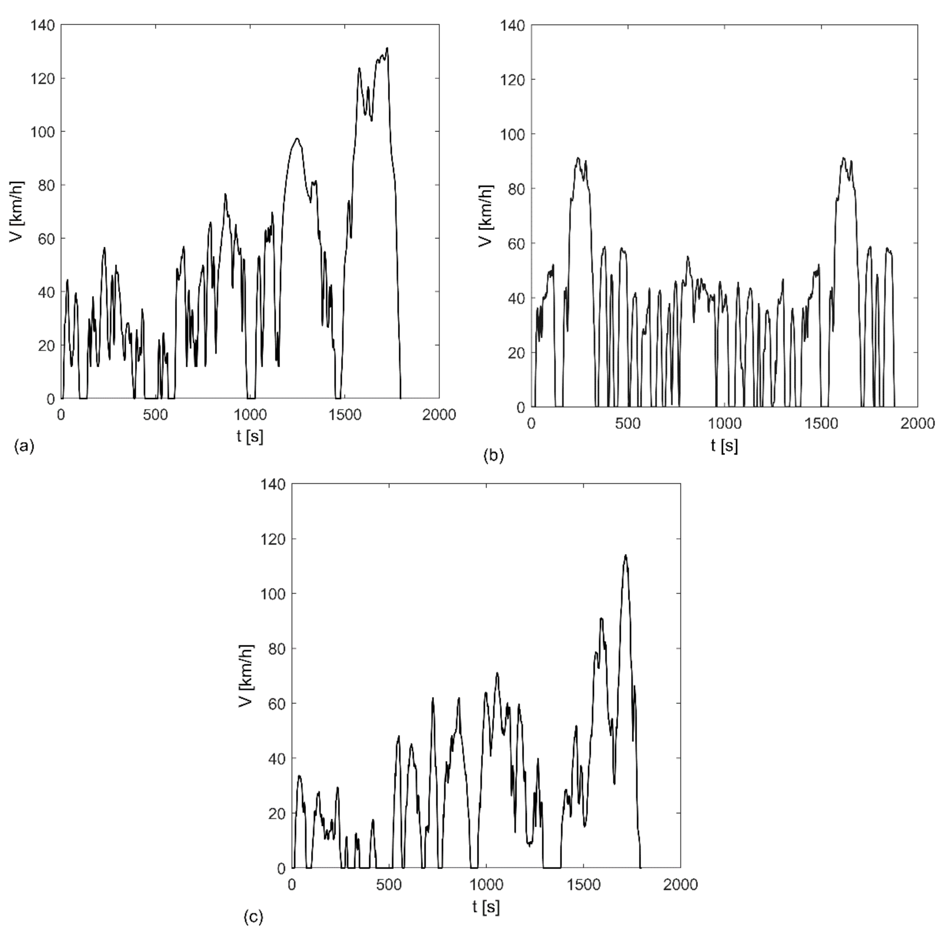
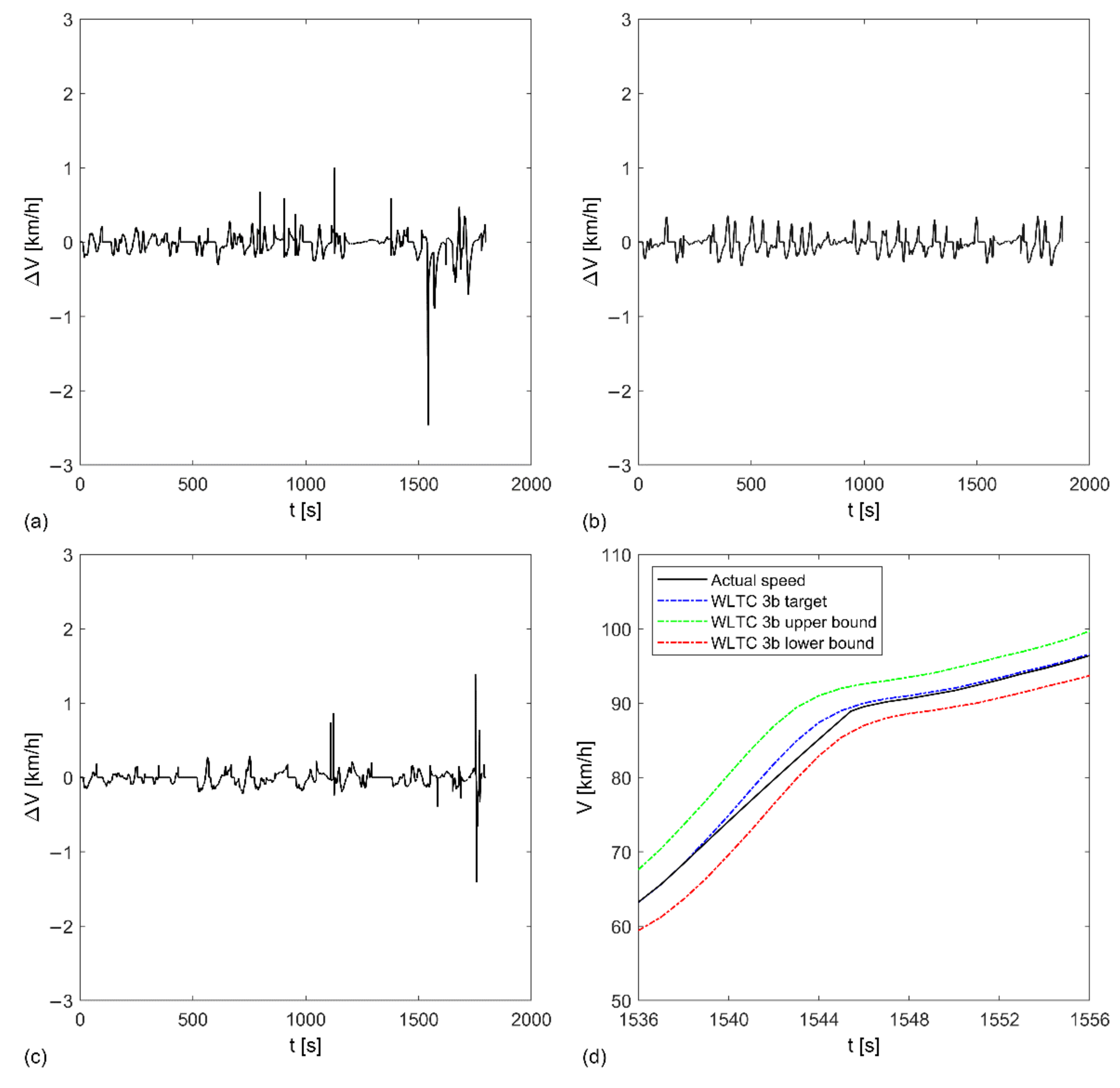
  • vehicle speed validation in WLTC 3b, FTP-75, and CLTC-P drive cycles,
  • pure electric range (BEV mode),
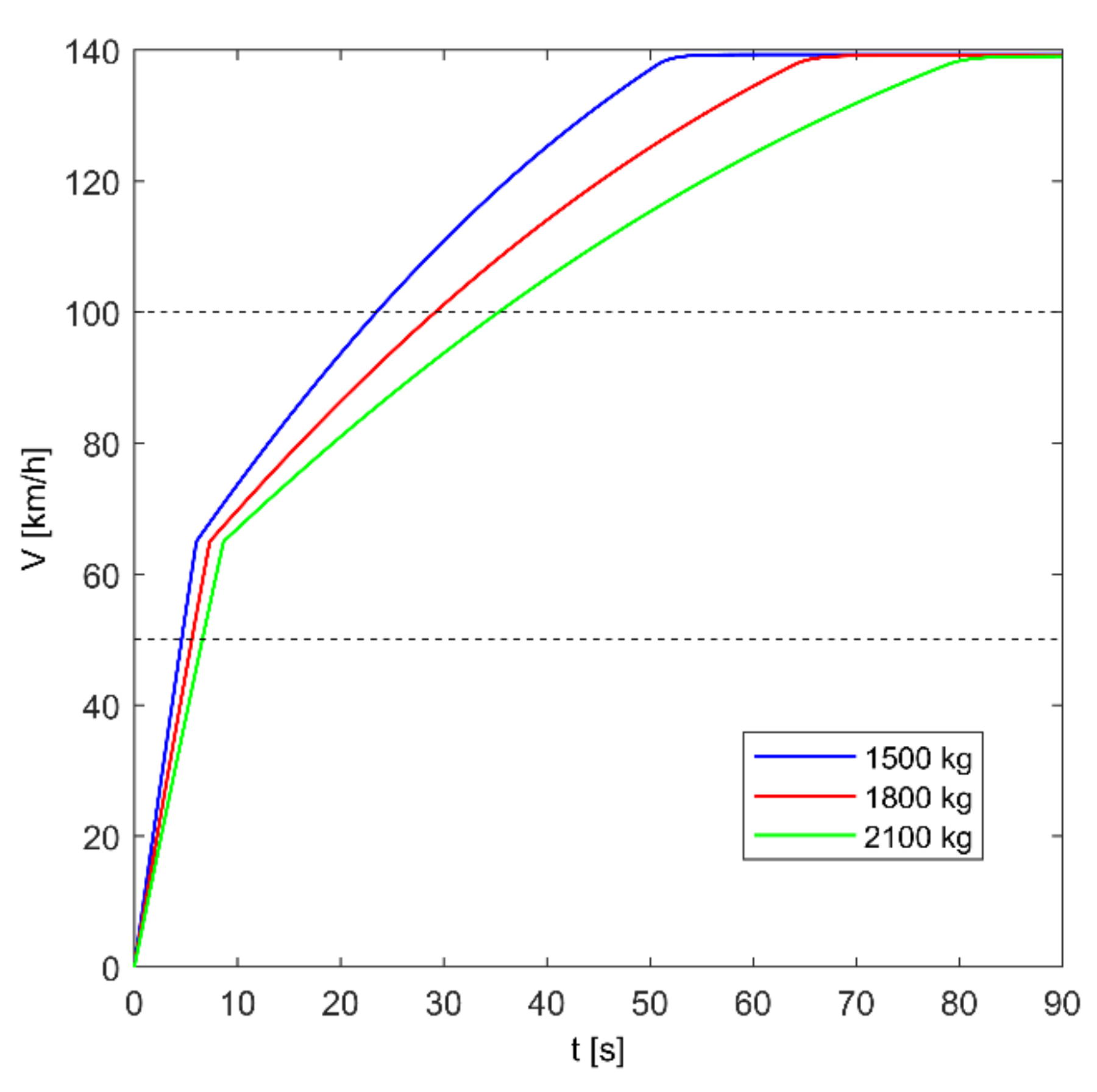
  • acceleration times,
  • validation of REX control strategy for multiple of range target values,
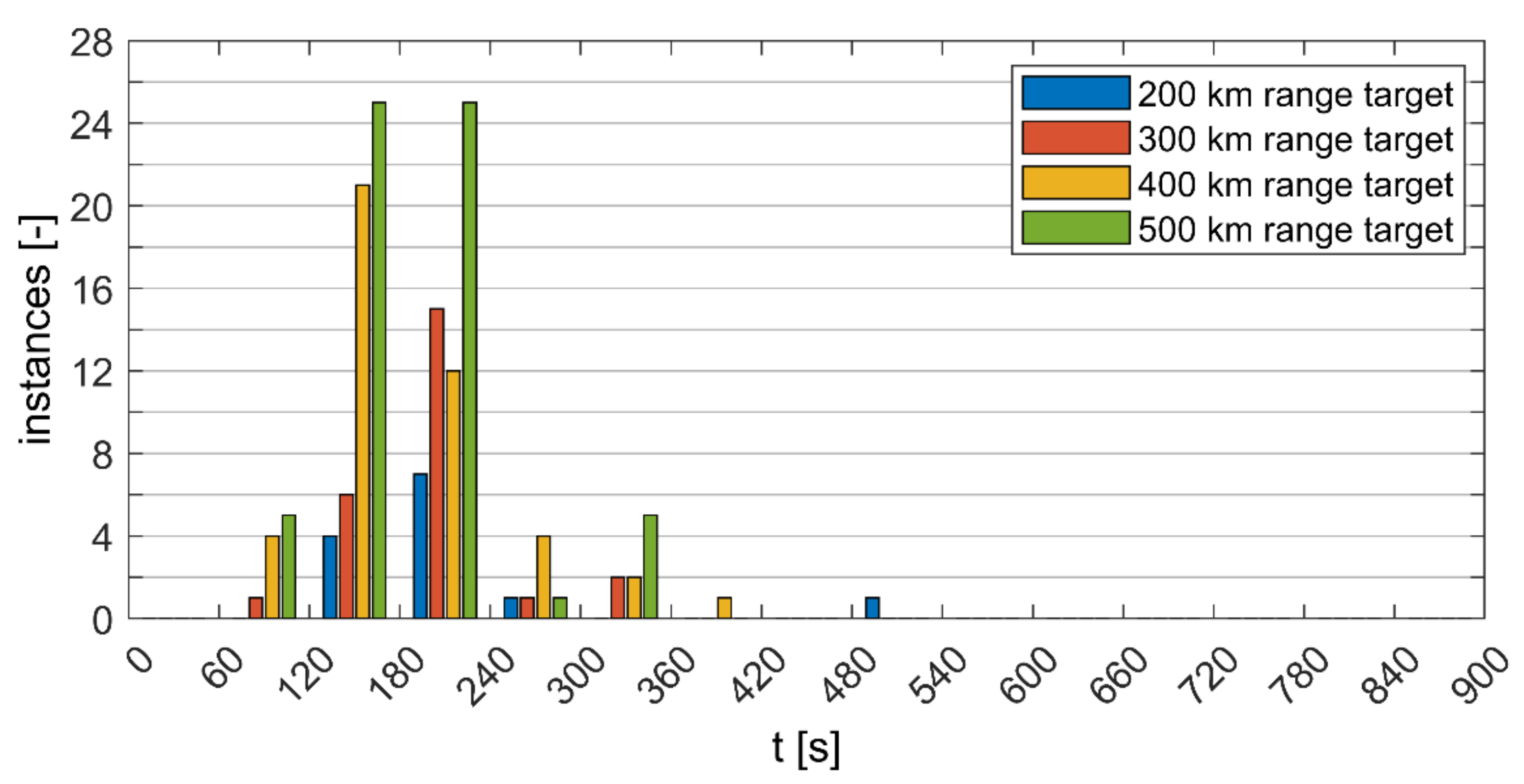
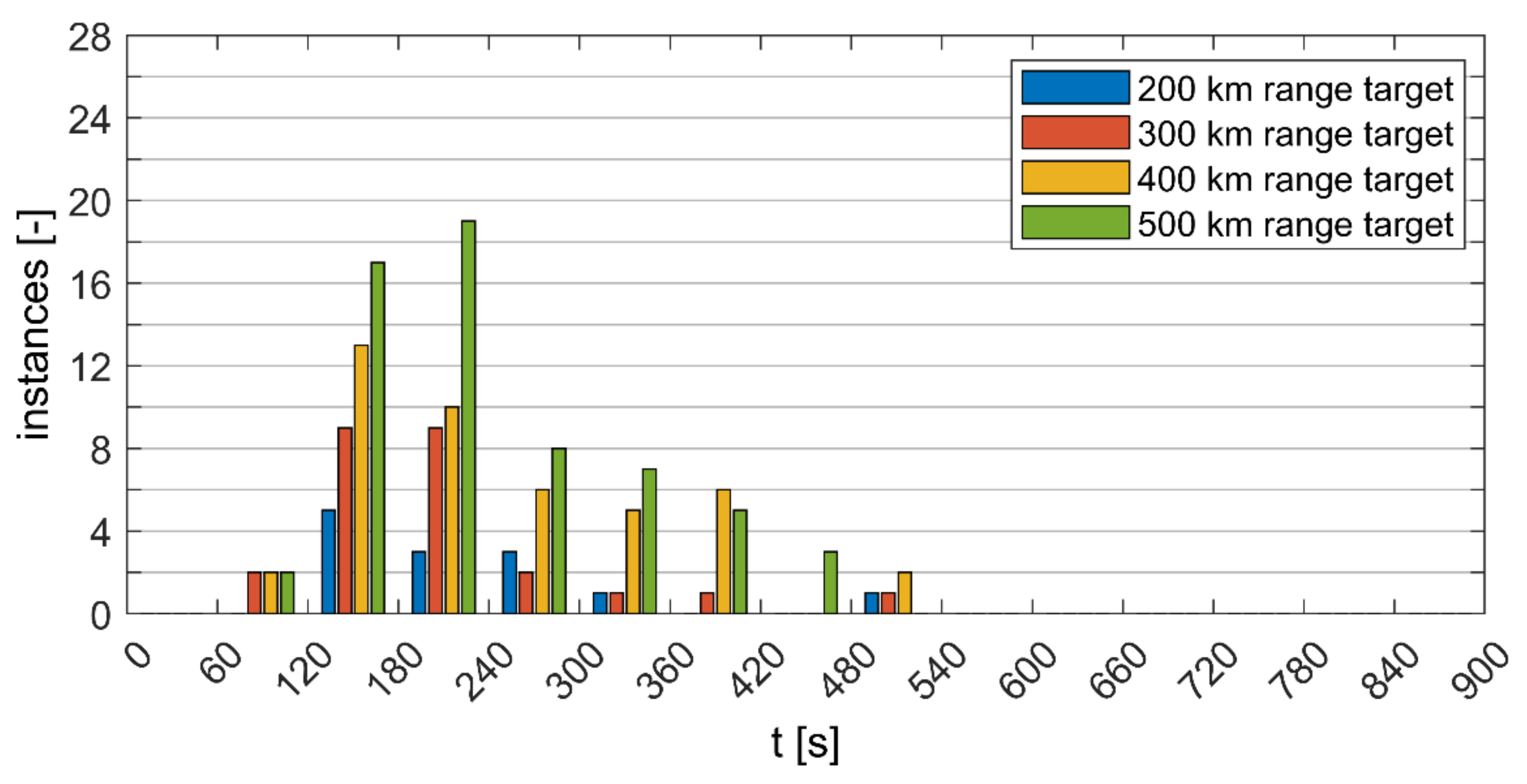
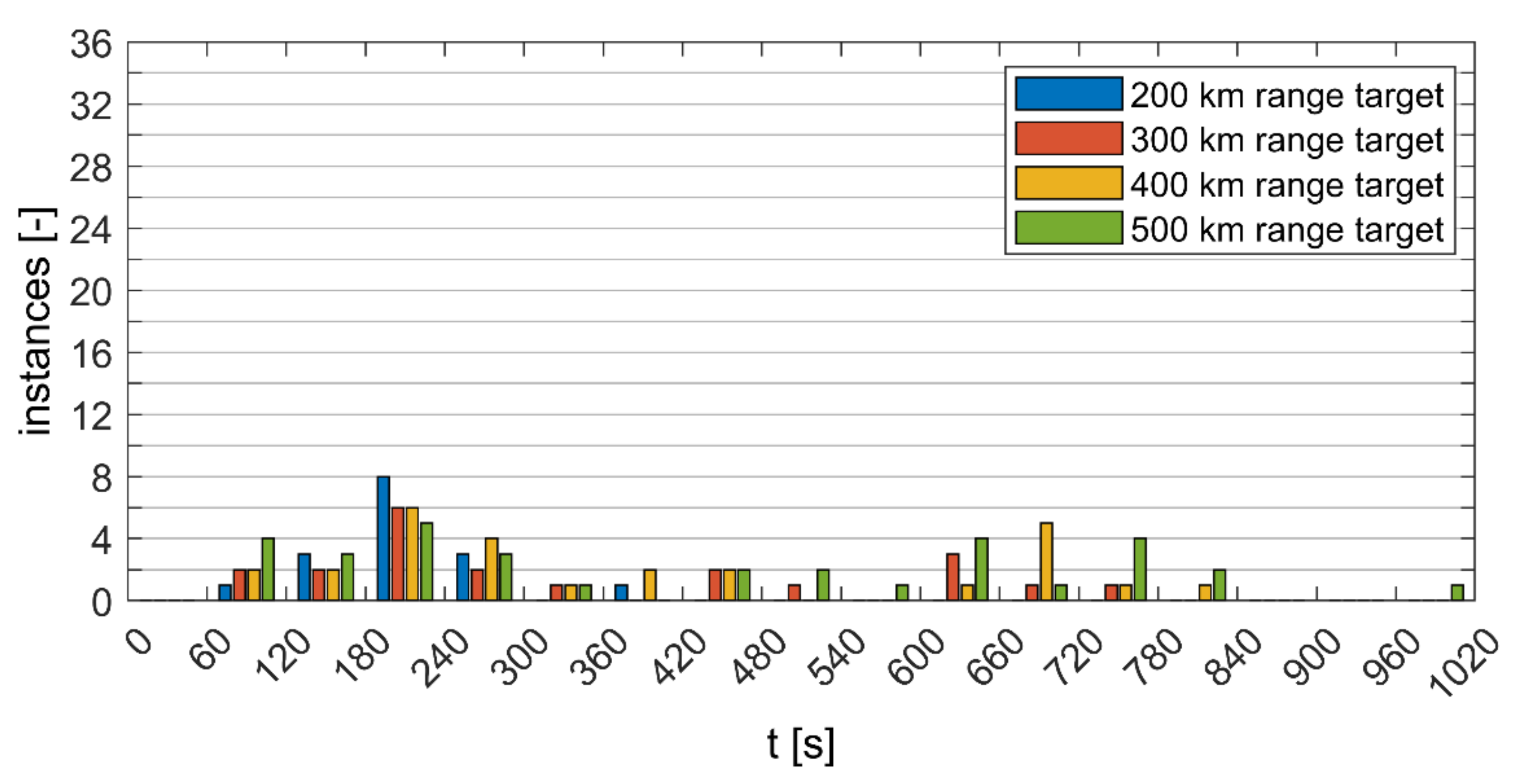
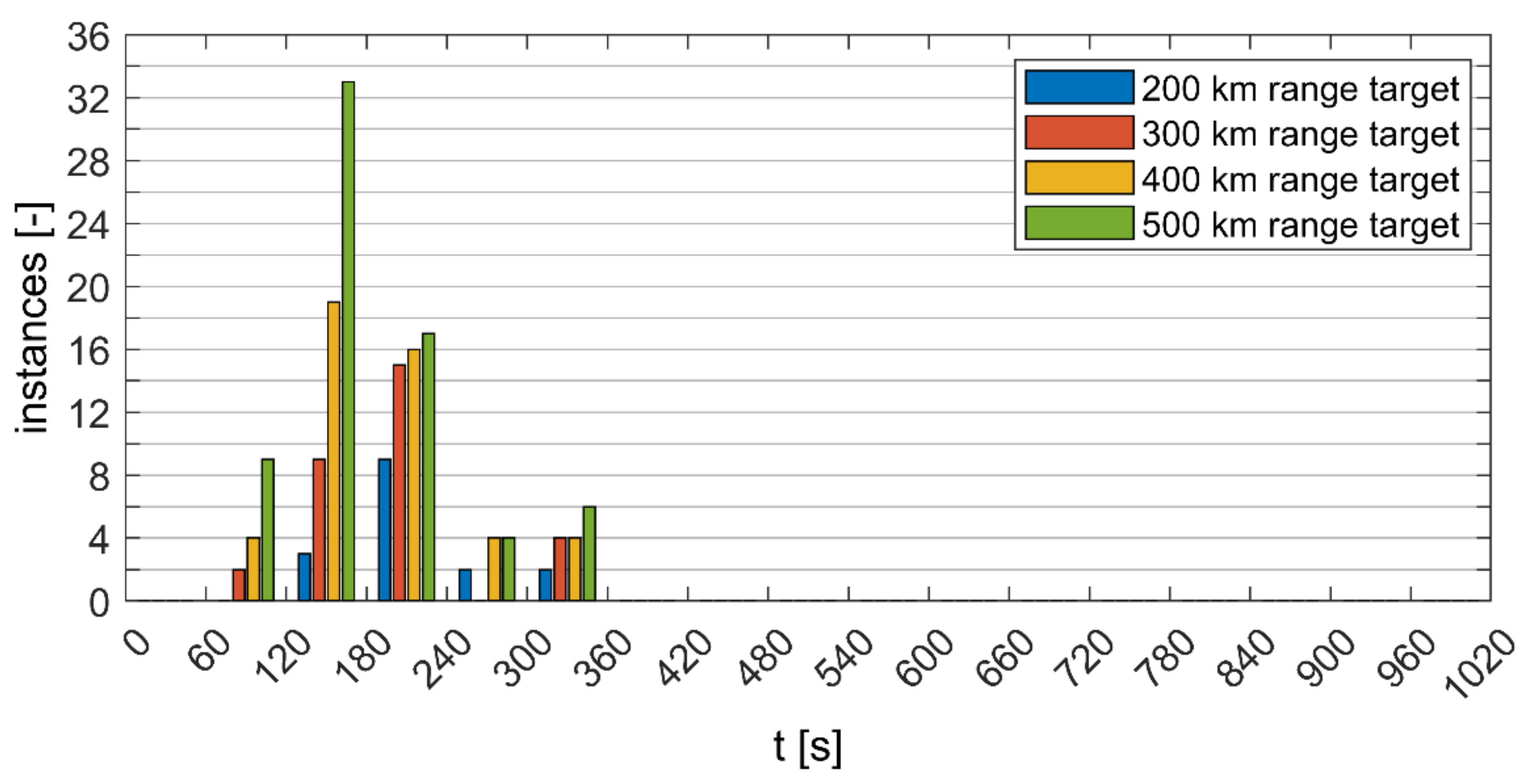
  • REX utilization metric and distribution of its engagement instances,
  • fuel consumption,
  • combined (fuel and electricity) CO2 equivalent emissions,
  • powertrain efficiency and specific energy consumption.
  • The study limitations are presented and finally, conclusions are made.

2. Materials and Methods

2.1. Vehicle Powertrain

The vehicle powertrain diagram is shown in Figure 1. The powertrain has the structure of a series Hybrid Electric Vehicle (series HEV). It is comprised of typical Electric Vehicle (EV) components (EM—Electric Motor, BAT—electrochemical battery pack, ECU—Electronic Control Unit, W—road wheels) and on-board REX. REX supplements vehicles with additional power. REX can be implemented by various energy carriers. These can be fuel cells or heat engines working together with an electric generator. In this work, the REX consisting of an internal combustion engine (ICE) powered by gasoline and an electric generator (G) is considered. Compared to the series hybrid, the EREV has a larger battery pack and a smaller power electric generator. Also, the control strategy, regarding the engine-generator unit and battery, is different from that of an HEV.

2.2. Vehicle Simulation Model

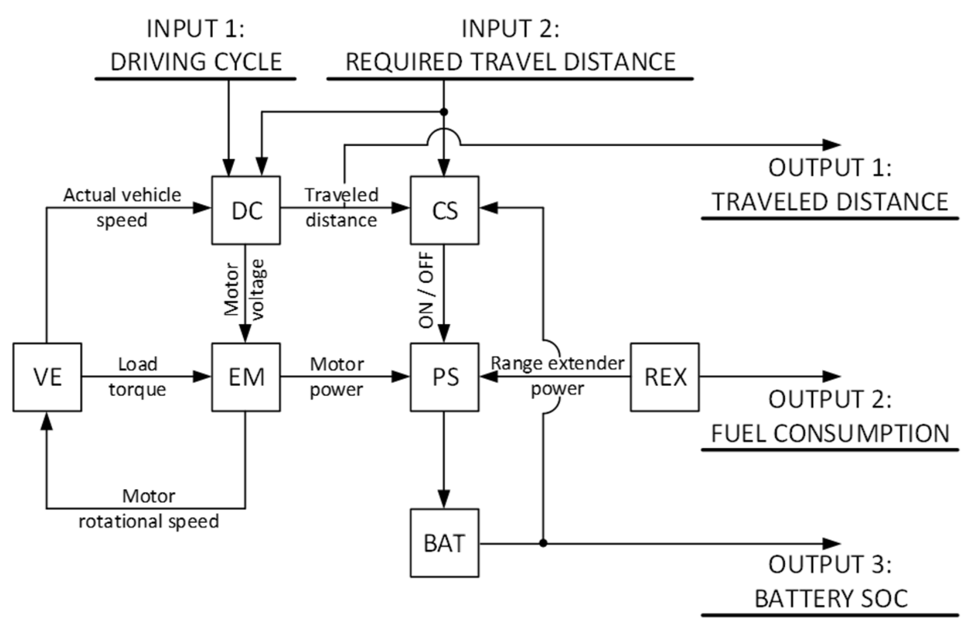
2.2.1. Model Topology

The vehicle model, shown in Figure 2, is comprised of elements representing essential components interacting with each other. Every component of the model has underlying mathematic formulas, which are used to calculate time-varying output quantities based on time-varying inputs.

2.2.2. Inputs and Outputs

The simulation model takes two main inputs: driving cycle and required travel distance. There are three main outputs: traveled distance, engine fuel consumption, and battery State of Charge (SOC).
A driving cycle is a series of data points representing requested vehicle speed versus time. For simulation, a set of 12 speed vs time data series is used. The first three data series are full driving cycles, namely: the Worldwide Harmonized Light-duty Test Cycle Class 3b (WLTC 3b), Federal Test Procedure (FTP-75) cycle, and China Light-Duty Vehicle Test Cycle (CLTC-P) for passenger cars [45,46,47]. Subsequent plots of these cycles are shown in Figure 3. Next three data series are specific parts of WLTC 3b and CLTC-P, namely WLTC 3b High 3-2 (3rd part of WLTC 3b), CLTC-P Phase 3 (3rd and last part of CLTC-P), and WLTC 3b Extra-High 3 (4th and last part of WLTC 3b). Last six data series are set to be constant speeds of 90, 100, 110, 120, 130, and 140 km/h.
The second input is the value of required travel distance (in other words value of traveled distance that should be achieved). EREV simulation runs are conducted for four values of requested travel distance (200, 300, 400, and 500 km), to check the performance of the proposed control strategy. The set value is the target for the final value of the traveled distance of the vehicle in a particular simulation, ideally achieved at the set SOC level.
The first output is the value of traveled distance. It is a time integral of vehicle speed achieved in the driving cycle.
The second output is fuel consumption. The vehicle has a range extender unit modeled using maps of Brake Specific Fuel Consumption (BSFC) versus range extender rotation speed and torque, and CO2 emission versus range extender speed and torque. These maps are the results of empirical research conducted by the authors [48]. Fuel consumption is calculated by integrating BSFC over time for given range extender rotational speeds and torques. The operating point is set accordingly to REX set power in the area of low BSFC (the BSFC map with engine point of operation is shown in Section 2.2.8 of the paper).
The third output is a battery SOC value. This value is calculated by the battery simulation model and described in the battery model section. The simulation run is stopped when the predetermined level of 0.15 battery SOC is reached.

2.2.3. Vehicle Body and Driveline Model

Forces acting on the vehicle in motion are:
  • tire rolling resistance,
  • air drag force,
  • and force of inertia of moving vehicle and rotating drivetrain components.
Equation (1) shows the sum of these forces, making total resistance force acting on the vehicle wheels. The rolling resistance force is constant and depends on vehicle mass m, gravitational acceleration g, and rolling resistance coefficient frr. Frontal air drag force is a function of air density ρ, vehicle frontal area A, drag coefficient cd, and momentary value of vehicle speed. The last three terms of Equation (1) represent the force of the inertia, dependent on vehicle acceleration a(t). This force is associated with vehicle mass m, wheels inertia Jw and EM rotor inertia Jm. The number of rolling wheels is given by nw, rd is the dynamic radius of tires, ηd is drivetrain efficiency, and i is a motor-wheels mechanical gear ratio.
Fr(t) = mgfrr + 0.5ρAcdv(t)2 + ma(t) + nwJwa(t)/rd2 + ηdsign[Fr(t)] Jmi2a(t)/rd2
External torque acting on the EM shaft is given by Equation (2).
Tmech(t) = [mgfrrrd + 0.5ρAcdv(t)2rd + ma(t)rd + nwJwa(t)/rddsign[Fr(t)]/i

2.2.4. Electric Motor Model

The electric motor is a three-phase Permanent Magnet Synchronous Motor (PMSM). Three-phase motor stationary coordinates a, b, and c, are referring to specific stator supply phases. But due to the complexity of describing electromechanical equations often Park’s transform is used. Stationary coordinates are transformed to direct axis–quadrature axis (d–q) coordinates (Figure 4).
In d-q coordinates supply voltages in d-q axes are given by Equations (3) and (4).
ud = Rmid + d(λd)/dt − pωmλq
uq = Rmiq + d(λq)/dt + pωmλd
where: id, iq—electric currents in d and q axes respectively, Rm—stator resistance, p—number of motor magnetic pole pairs, ωm—rotor speed, λd, λq—flux linkages for corresponding axes. The electromagnetic torque (Tm) of PMSM is given by Equation (5).
Tm = (3/2)p(λdiq − λqid)
Flux linkages are given by Equations (6) and (7).
λd = Ldid + λf
λq = Lqiq
where: Ld, Lq—motor inductance in d and q axes respectively, λf—magnetic flux linkage due to permanent magnets.
For PMSM assumption is made that the magnetic circuit is symmetrical and inductances Ld and Lq are equal to motor inductance Lm. For ease of model implementation in simulation, a set of Equations (3)–(5) are rewritten as given by Equations (8)–(10).
d(id)/dt = ud/Lm − Rmid/Lm + pωmiq
d(iq)/dt = uq/Lm − Rmiq/Lm − pωmid − pωmλf/Lm
Tm = (3/2)piqλf
Motor current and voltage are given by Equations (11) and (12).
im = sqrt(id2 + iq2)
um = sqrt(ud2 + uq2)
In the simulation, the motor is controlled by adjusting voltages in d-q axes so that vehicle follows a given cycle speed trajectory. Moreover, the zero d-axis current control strategy (ZDAC) is implemented [49]. Both speed and current control are realized by PI controllers.
Computation of rotational speed ωm can be performed by solving the Equation (13) of motor rotor motion:
Tmηm − Tmech = Jmd(ωm)/dt
where: Tmech—external load torque on the motor shaft, ηm—motor mechanical efficiency, Jm—rotor inertia.

2.2.5. Battery Model

The battery has two values of SOC set. At the start of simulation run, SOC is equal to 0.9 and at the end of the simulation, SOC is equal to 0.15 (this is the trigger for the simulation run ending).
The battery SOC is calculated by comparing momentary battery charge outflow and inflow, to nominal battery full charge Qbn and then subtracting the resultant value from the initial SOC value (Equation (14)). Battery charge is calculated by integrating battery current Ib over time. Battery efficiency is included in equation via Peukert’s coefficient β, which relates momentary battery current to nominal battery current Ibn.
SOC = SOC0 − (1/Qbn)∫(Ibkβ)dt
where kβ is given by Equation (15):
kβ = (Ib/Ibn)^[(β − 1)sign(Ib)]
Ib is calculated using the equivalent circuit equation of battery voltage Ub (Equation (16)), with an electromotive force of single battery cell ebc as a function of SOC, and internal resistance of single battery cell Rbc also as a function of SOC. These parameters can be expressed in a form of polynomial functions [50,51]. The battery is made of many cells, where nbs is a number of series cell connections, and nbp is a number of parallel cell connections.
Ub = nbs[ebc − Rbc(Ib/nbp)]
To relate battery current with battery power load and therefore complete the current calculation iteration loop, Equations (14) and (16) must be solved in conjunction with Equation (17).
Ib = Pb/Ub

2.2.6. Range Extender Model

Range extender provides additional electricity to the electric powertrain by using some source of energy. The REX model is based on laboratory REX which comprises Honda IGX440 dual fuel—gasoline/Liquefied Petroleum Gas (LPG)—internal combustion engine (in this study gasoline-only operation is presented) and KOMEL PMGgi132M4C permanent magnet synchronous generator. Such a setup could be mathematically represented as a matrix of values of the required quantity. In this case, a map of BSFC is a function of engine rotational speed and torque [52,53]. The map is derived from test bench REX measurements [48]. The model used in the simulation has REX scaled up from the laboratory REX, keeping the same rotation speed range, but having 3.4× higher torque than the laboratory REX (map of BFSC with the point of operation is shown in Section 2.2.8). Each REX start carries a penalty given by the amount of 10.2 cm3 of consumed fuel [54].

2.2.7. Power Summing Node and REX Control Strategy

The power summing node in EREV is an electric power converter. This device can be modeled based on its electric circuit. But the topology of such a device for automotive application is complex since it is fulfilling multiple functions: supplies EM from the battery, distributes REX power to the battery and the EM, and transfers power from EM to the battery during regenerative braking.
To simplify the problem of modeling the power summing node, the power converter is treated as a three-way power summing node with the efficiency of power flow paths. Equation (18) describes power flow with the inclusion of efficiencies within the power summing node:
Pmηcmsign(Pm) + Pbηcbsign(Pb) + Pgηcg = 0
where: Pm—EM power at its terminals, Pb—battery power at its terminals, Pg—REX power at its terminals, ηcm—power converter efficiency for energy transfer between the EM terminals and the power summing node, ηcb—power converter efficiency for energy transfer between battery terminals and the power summing node, ηcg—power converter efficiency for energy transfer between the REX terminals and the power summing node.
A schematic representation of multiple functions of the power summing node is shown in Figure 5, with specific cases of power flow listed in Table 1.
The goal of the control strategy is to use all available battery SOC (within its set limits) and extend the vehicle range to obtain a range value of R. The R-value should be set by the user or for example by an infotainment system integrating satellite maps, based on the required trip distance to a given destination. REX control strategy triggers its state to on or off. This two-state control links battery SOC and vehicle range to determine suitable on and off trigger levels. These levels are two vehicle speeds, VON and VOFF. When vehicle speed crosses VON (trigger level up) the REX is enabled and when vehicle speed crosses VOFF (trigger level down) the REX is disabled. Values of VON and VOFF are time-dependent and are governed by the PI regulator. Control variable u(t) determines trigger levels (Equations (19) and (20)).
VON(t) = u(t)
VOFF(t) = u(t) − VD(te)
VD is the dead zone speed range, the constant difference between VON and VOFF. To prevent REX from running for very short periods, the VD value is calculated during the REX engagement period as a function of engagement instance time te, given by Equation (21):
VD(te) = VD0 + max(0; ((2 × TB − te)/(2 × TB)) × (2 × VMAX − VD0))
where: VD0—base dead zone range of 40 km/h, TB—preferred minimum REX engagement time set to 120 s, VMAX—vehicle to a speed of 140 km/h. The presented dead zone widening limit instances of REX running shorter time than TB.
The desired process value r(t) is the range in kilometers that the vehicle should travel spending charge from the battery, resulting in the momentary value of SOC(t). The measured process value y(t) is the actual range traveled, resulting in a momentary value of SOC(t). Error e(t) is the difference between r(t) and y(t).
Process value is defined by Equation (22):
r(t) = R(1 − SOCEND)/(SOC0 − SOCEND)
where R is a set range that should be obtained discharging battery from SOC0 to SOCEND. Here R, SOC0, and SOCEND are assumed to be constant, not changing during driving, therefore process value r is also constant. But in other cases, not presented here, these values could be changed during the drive, for example by a user.
The relation between s(t) and SOC(t) is controlled to be linear, which is described by function y(t) (Equation (23)).
y(t) = (s(t) + r(1 − SOC0)/(1 − SOCEND))/((1 − SOC(t)/1 − SOCEND)
where: s(t) is the traveled distance. At the end of the drive (SOC(t) = SOCEND) s(t) should be close to set range R.
The PI regulator formula (Equation (24)) requires tuning KP and KI values.
u(t) = KPe(t) + KI∫e(t)dt
For the tuning of KP and KI values, a simulation experiment was set up. The vehicle speed was set to a constant 70 km/h (half of the top speed) and set driving range R to 400 km. In this experiment, the KI term was set to 0 and the KP term was variable. The periodic changes of process value y(t) were observed. The KP value was modified so that y(t) was changing in the range of r(t) ± 0.01R, which gave the value of KP0. Then the period T0 of oscillations was measured as an average over the driving time. The resultant values of KP and KI (Table 2) were calculated by formulas given by the Ziegler-Nichols heuristic method, assuming that KP0 is equal to Ku and T0 is equal to Tu [55].

2.2.8. Test Object Model Parameters

EREV in question is a mid-size, Leisure Activity Vehicle (LAV). EREV powertrain structure is a series hybrid with plug-in capability. The structure of the powertrain is described in the authors’ previous papers [11,48]. The operation mode implies that the battery will be discharged at end of the driving cycle. Moreover, the engine-generator unit has power sufficient to extend the driving range, but not high enough to recharge the fully onboard battery during the drive. This approach leads to higher usage of battery electric energy storage and lower use of a generator. Therefore, a smaller amount of fuel can be consumed and smaller amount of tailpipe pollutants emitted.
The main vehicle parameters used in the simulation are shown in Table 3, excluding traction wheels parameters which are included in Table 4. The vehicle mass of 1500 kg, with two passengers and luggage, represents a typical use case scenario for driving in mixed conditions and is also applicable to road trips outside city limits. Higher loads are also included, represented by masses of 1800 kg and 2100 kg. The vehicle has two-speed mechanical transmission.
The electric motor of the vehicle is a permanent magnet synchronous type (PMSM). It is highly efficient and has the power required to fulfill typical driving needs (Table 5). Its maximal value of rotational speed with selected transmission 2nd ratio allows achieving a vehicle top speed of 140 km/h.
The battery pack comprised of 108 cells made in lithium-ion technology (Table 6) allows for a significant electric driving range. The extreme values of the battery State of Charge (SOC) are not used due to the risk of over-charge, over-discharge, and lower efficiency operation, therefore the risk of lower operation life.
The power summing node has its efficiency values (ηcg, ηcm, and ηcb) set to 96%. Additionally, there is an auxiliary load of 500 W, which represents an average electric power consumption of vehicle systems.
Range extender comprised of a small internal combustion engine and permanent magnet synchronous generator has working point set in the area of its low specific BSFC (Table 7). This provides low fuel consumption and low emissions but requires switched on-off operation governed by a control algorithm. It must be controlled in such a way that provides expected range extension, but at the same time allows the battery to discharge to the required SOC level at the end of the drive. The BSFC map of REX with its operation point is presented in Figure 6.

2.3. Simulation Tests Conditions

Simulation to be practical and to give a replicable test run results most certainly must have constraints, simplifications, and set up characteristic values not only in the simulation itself but also in the computer software running the simulation. The subsection below presents the main assumptions of simulation and lists also simplifications and omissions in the description of physical phenomena describing EREV and its operation. The next subsection focuses on computer software settings and how to achieve CO2eq emission values from test run results.

2.3.1. Main Assumptions of Simulation

The test conditions are determined by a set of assumptions:
  • vehicle follows test cycle speed profile,
  • vehicle mass is constant during the simulated drive,
  • influence of weather conditions (wind, rain, atmospheric pressure, temperature) on the vehicle is neglected,
  • there is no road gradient,
  • parameters of REX fuel are constant,
  • there is no delay in REX start,
  • vehicle speed control is the same across all simulated driving cycles,
  • thermal phenomena in the motor, controller, and battery are neglected—it is assumed that cooling the vehicle components is sufficient,
  • no motor torque and speed overloading,
  • instantaneous gear changes,
  • no loss of grip between tires and road surface.

2.3.2. Software and Simulation Goals

LAV model was implemented to the Matlab-Simulink® software and simulated with a fixed iteration step of 0.01 using an ODE45 solver (ordinary equations solver that implements a Runge-Kutta method), with relative and absolute tolerances set to 1 × 10⁻⁷.
The goals of the simulation were reliable calculations of various metrics, including CO2eq emission across different range extension values. Fuel consumption value carried additional information. The simulation also allows for precise calculation of actual driving range for specific set range scenarios, as well as battery energy expenditure per 100 km.
Additionally, three use case scenarios regarding electricity mix were presented, due to vast differences in CO2eq emission of electricity production, the first case assumes that battery electricity is produced in Poland, with greenhouse gas emission intensity of electricity generation of 709.8 gCO2eq/kWh, the second case assumed average EU-27 greenhouse gas emission intensity of electricity generation of 230.7 gCO2eq/kWh, and the third one assumed that electricity for battery charging was produced in Sweden at 8.8 gCO2eq/kWh [56]. It is assumed that the battery must be charged from the grid before the trip from 0.15 SOC to 0.9 SOC. Therefore total CO2eq (battery electricity and gasoline) emission can be calculated and compared. Gasoline emits 66.8 CO2eq/MJ [57]. CO2eq emission of simulation run is calculated as a sum of single grid charging CO2eq emission and CO2eq emission from combusted fuel in REX.
For such a setup, including various input permutations, a minimum of 180 simulation runs must be performed (not counting multiple test runs leading to simulation model improvements). Having enough results enables us to present insightful information on EREV operation.

3. Results and Discussion

3.1. Driving Cycles Speed Validation

Main test conditions are determined by chosen driving cycles, which are WLTC 3b, FTP-75, and CLTC-P. Every cycle has its speed profile which the vehicle should follow. To verify how this condition is met Figure 7a–c shows plots of speed differences between simulation results of vehicle speed and speed of each cycle. Figure 7d shows zoom at the highest difference between the test cycle speed and actual vehicle speed (WLTC 3b). The vehicle speed stays within the required bounds.
Each cycle validation is performed with the same vehicle settings. The resulting speed differences, calculated as standard deviation, are presented in Table 8. Values of the standard deviation of speed show that between three cycles, the WLTC 3b driving cycle has the largest value of this measure, suggesting that it is the most demanding one in terms of speed changes. All presented values can be considered as low because cycle speed is tightly followed in all three cycles.

3.2. Pure Electric Drive Range and Acceleration Times

Pure electric drive range results were included because the tested powertrain has such capability and it is preferred to be used if possible in any drive cycle because it avoids pollutant emissions from combustion engine (Table 9, Table 10 and Table 11). The range values in BEV mode show that WLTC 3b range is between 14.7 and 17.6% lower than in FTP-75 and between 12.0 and 14.5% lower than in CLTC-P. An increase of vehicle mass from 1500 kg to 2100 kg reduces the range by 14.7% in WLTC 3b, 17.6% in FTP-75, and 17.1% in CLTC-P.
Results for fragments of WLTC 3b and CLTC-P drive cycles, namely WLTC 3b High 3-2 and CLTC-P Phase 3, have higher range values in the case of WLTC 3b High 3-2 in comparison to whole WLTC 3b, and lower range values in the case of WLTC 3b High 3-2 in comparison to whole WLTC 3b. But for higher speed testing the WLTC 3b Extra-High 3 is resulting in significantly lower range values and for all three mass variants resulting range is less than 90 km, showing the lowest vehicle autonomy.
Results of the BEV mode range included in Table 11 are for constant speed diving, with relatively high speeds. Firstly, the results show a great reduction of range with increasing speed, up to 45.8% (between 90 km/h and 140 km/h, for a vehicle mass of 1500 kg). When driving at high speed (140 km/h) range loss is even greater, topping 57.5%, when compared with the FTP-75 drive cycle (average speed of 34.1 km/h). The percentage of range loss due to the increase of vehicle mass (form 1500 kg to 2100 kg) diminishes with an increase in speed and it is in the range of 13.2–8.1% (90–140 km/h).
Acceleration times for three variants of vehicle mass are presented in Table 12. Corresponding plots are shown in Figure 8. Change in acceleration occurring between 60 km/h and 70 km/h is the result of a gear change from first to second speed. The resultant acceleration times in first gear are in line with gasoline-powered city cars (typically 4–5 s for 0–50 km/h). Second ratio acceleration is much less, but bear in mind that for the powertrain, the motor torque overloading was not considered. Overloading in most case scenarios is possible to some degree, but due to a high number of variables influencing the final results, it was decided to stick with nominal motor parameters.

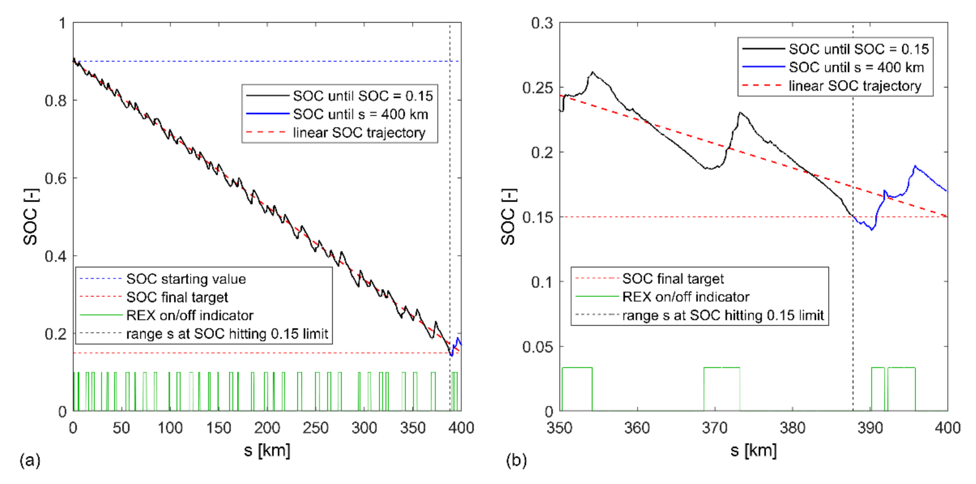
3.3. REX Control Strategy Validation for Range Targets

The control strategy should assure 15% SOC at a specified target regardless of cycle and load. But due to the dynamic nature of motor power demand, the momentary SOC drop could be so high that it may not be compensated by REX engagement. In another case, REX start, due to the nature of PI control, can be slightly delayed, and similarly, SOC could drop below 15%. This however occurs close to the target range and it does not mean that the target cannot be obtained. It simply means that at the target range SOC will be slightly below 15%. Table 13 shows the values of traveled distance and 15% SOC, for specified range targets and different driving conditions. The percent difference from the range target is in parentheses. Vehicle mass is set to 1500 kg. Results for vehicle masses of 1800 kg and 2100 kg are included in Appendix A, Table A1 and Table A2.
The results show the average percent difference between range target and traveled range from −0.51% (for 1500 kg) to −1.34% (for 2100 kg). Standard deviation of this metric ranges from 1.70% (for 1500 kg) to 2.18% (for 2100 kg). The highest observed range discrepancies at different mass levels were −13.9 km (WLTC-3b, 1500 kg, 2.79% short of 500 km target), −24.5 km (CLTC-P, 1800 kg, 4.91% short of 500 km target), −38.8 km (WLTC 3b, 2100 kg, −7.77% short of 500 km target). It may seem like this should be a problem, but in reality, most certainly would not be. For example in the last case presented above (high range discrepancy of −38.8 km) when the vehicle runs further and obtains eventually the range target of 500 km, SOC dips to a minimum of 13.2% (below 15% process value final target) and finish the run at 13.3% SOC. This is not ideal, but for outlier cases it is acceptable. The average range error across all tests where range could be obtained was −1.04% with 1.87% standard deviation, and the mean square error was 2.13%.
Another case explaining strategy operation is presented below. The strategy operation regarding SOC(t) as a function of the traveled range is shown in Figure 9a,b. Chosen simulation results are for the range target of 400 km for the FTP-75 driving cycle. It shows that even if SOC drops to process variable final target (15%) and at the same time traveled range s is short of the target value (here less than 400 km), the vehicle can obtain target range still, but with slight SOC deviation.

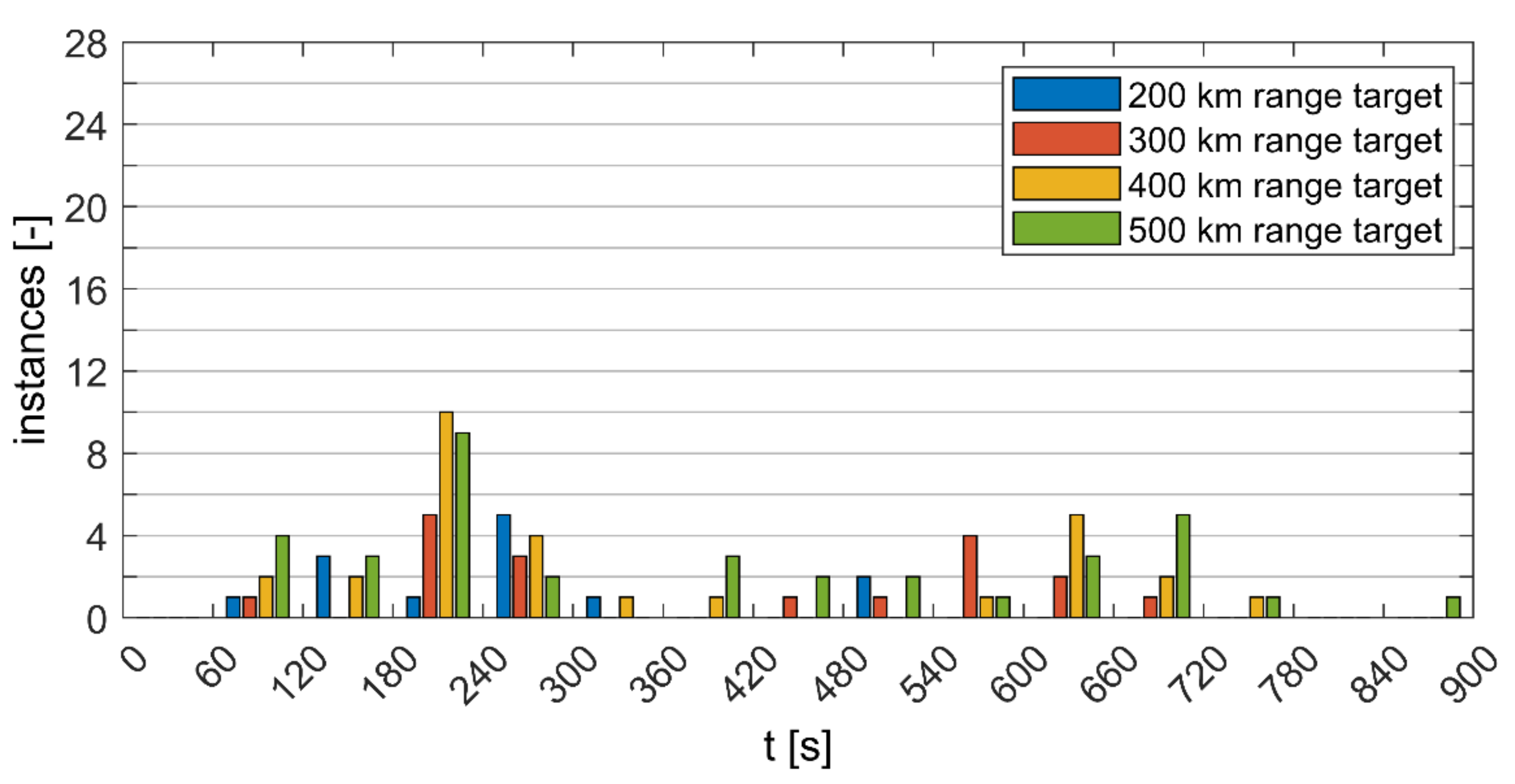
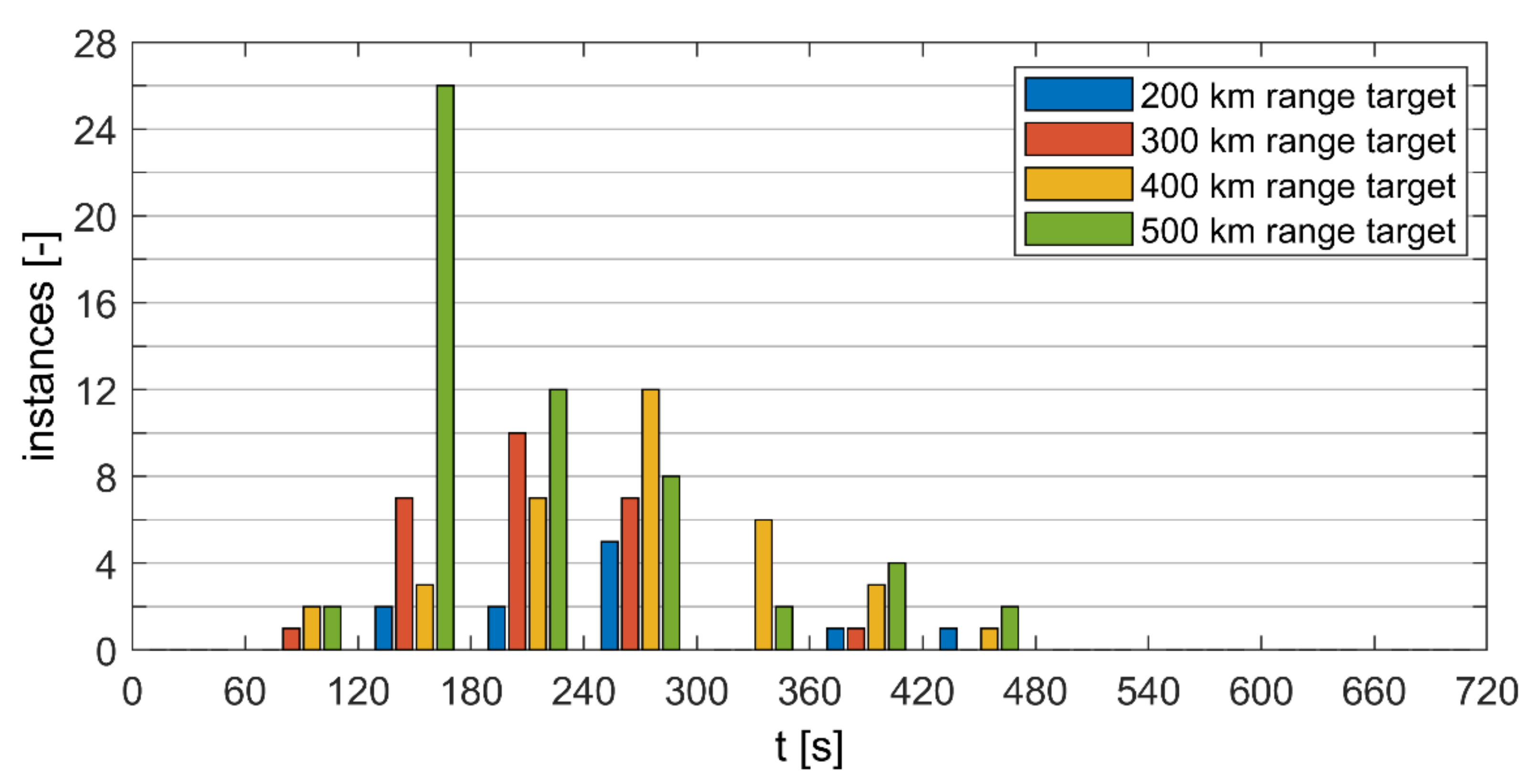
3.4. Range Extender Utilization

This subsection presents a selection of results showing how REX is utilized in WLTC 3b, FTP-75, and CLTC-P driving cycles. Figure 10, Figure 11 and Figure 12 show bar graphs of numbers of instances when REX was engaged, binned by the engagement time. Every bin counts four color-coded simulation runs for range targets of 200, 300, 400, and 500 km. Vehicle mass is 1500 km. Results for higher masses are presented on graphs in Appendix B, Figure A1, Figure A2, Figure A3, Figure A4, Figure A5 and Figure A6. The resultant distribution of REX running instance times shows that for WLTC 3b this distribution is more flat, leading to many instances spanning multiple minutes. For FTP-75 and CLTC-P these distributions are more concentrated and closer to the mean. In all cases, there is a low number of instances with the generator running below 120 s, which was a “soft limit” of shorter engagement timespan value. There are no instances when REX runs less than 60 s at a time.
Table 14 shows a summary of data presented in Figure 10, Figure 11 and Figure 12 and Appendix B, Figure A1, Figure A2, Figure A3, Figure A4, Figure A5 and Figure A6, giving average REX single instance running time and a total number of engagements (in parentheses) for WLTC 3b, FTP-75, and CLTC-P. Range targets are 200, 300, 400, and 500 km, and vehicle mass is 1500 kg. Results for masses of 1800 kg and 2100 kg are included in Appendix A, Table A3 and Table A4. Average REX run instance time and the number of engagement instances tend to increase with increasing range target. Also, an increase in vehicle mass tends to increase these values. This indicates that the REX control strategy reacts to the changing simulation inputs, providing proper range extension.
Table 15 shows the utilization of REX in the share of total driving time. Columns represent range targets and rows various driving cycles plus constant speed drive. Vehicle mass is set to 1500 kg. Results for vehicle masses of 1800 kg and 2100 kg are included in Appendix A, Table A5 and Table A6. REX utilization shows clearly the limit of the ability of REX to provide sufficient energy to obtain the range target. When the utilization approaches close to 100% there is no means to perform correct EREV powertrain control utilizing the proposed strategy. There are few cases for higher vehicle speeds when the EREV range can be meaningfully extended (in absolute terms—kilometers).

3.5. Fuel Consumption

Fuel consumption values, in dm3 per 100 km, are obtained for four different target range values and three vehicle masses (Table 16, Table 17 and Table 18). Results for other driving cycles and constant driving speeds are included in Appendix A, Table A7, Table A8, Table A9, Table A10, Table A11, Table A12, Table A13, Table A14 and Table A15. Bolded values indicate that REX is engaged once and working constantly, and a range target cannot be obtained. Values in parentheses show the actual range value when SOC dropped to 15%. These results show that from three standard drive cycles the lowest fuel consumption per 100 km is obtained for FTP-75 (the lowest overall observed value is 1.37 dm3/100 km for a range target of 200 km and mass of 1500 kg, the highest FTP-75 value is 4.59 dm3/100 km for 500 km range target and mass of 2100 kg), followed by CLTC-P (higher between 3.3 and 16.0%) and WLTC 3b (higher between 20.1 and 73.2%). Fuel consumption increases with traveled distance and vehicle mass, and tops out for WLTC 3b Extra-High 3 drive cycle at 6.85 dm3/100 km (Table A9, Appendix A).

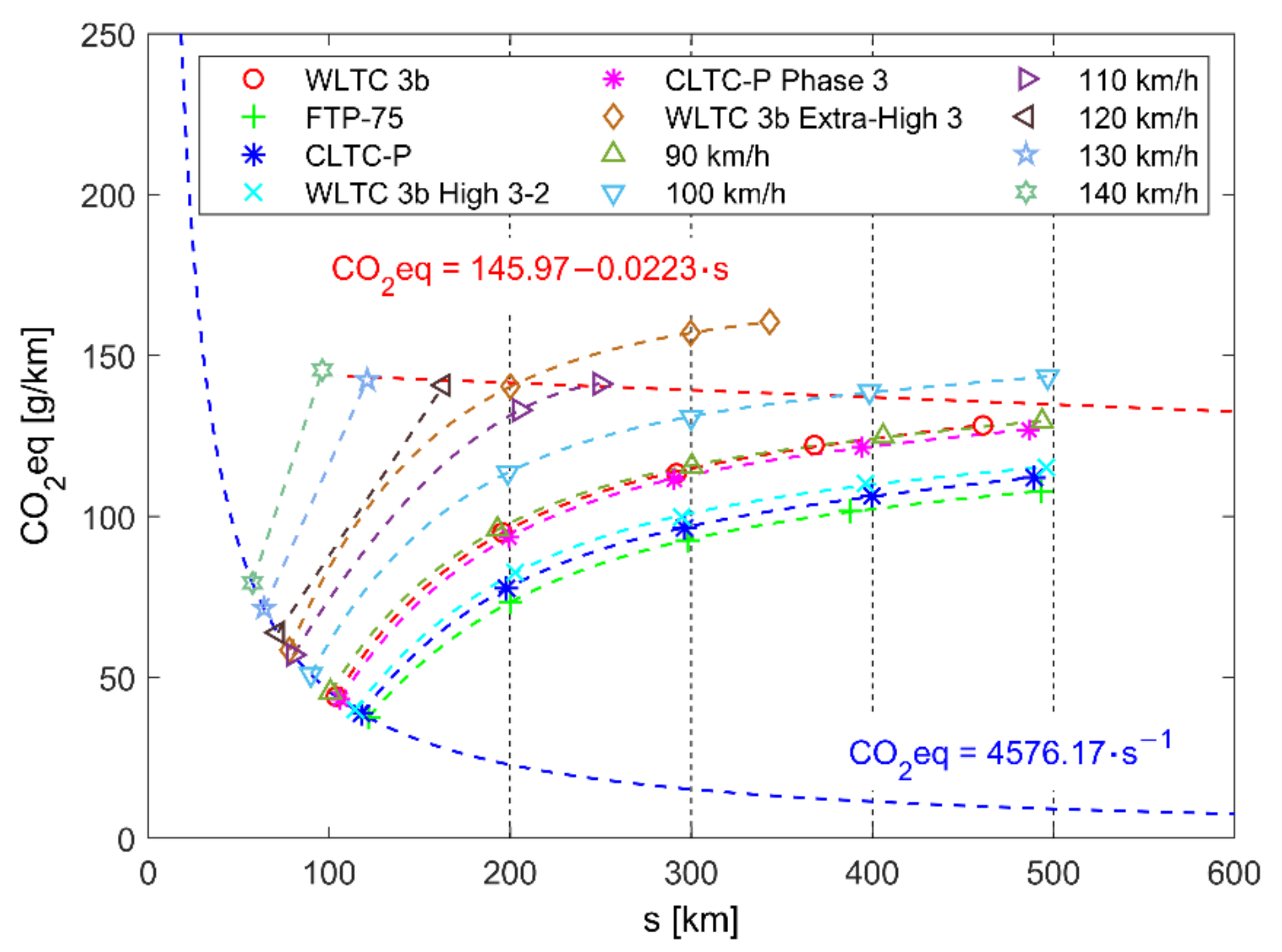
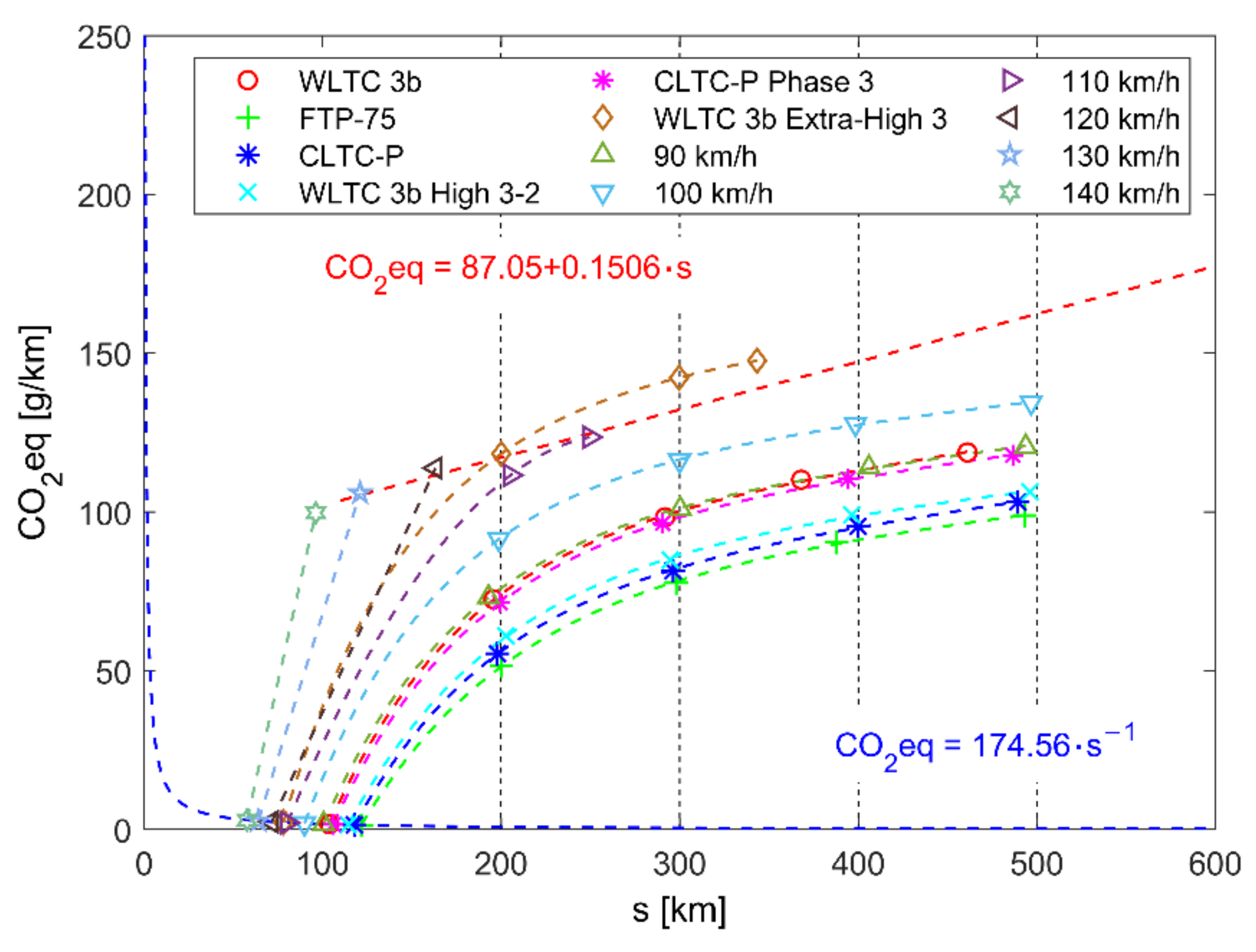
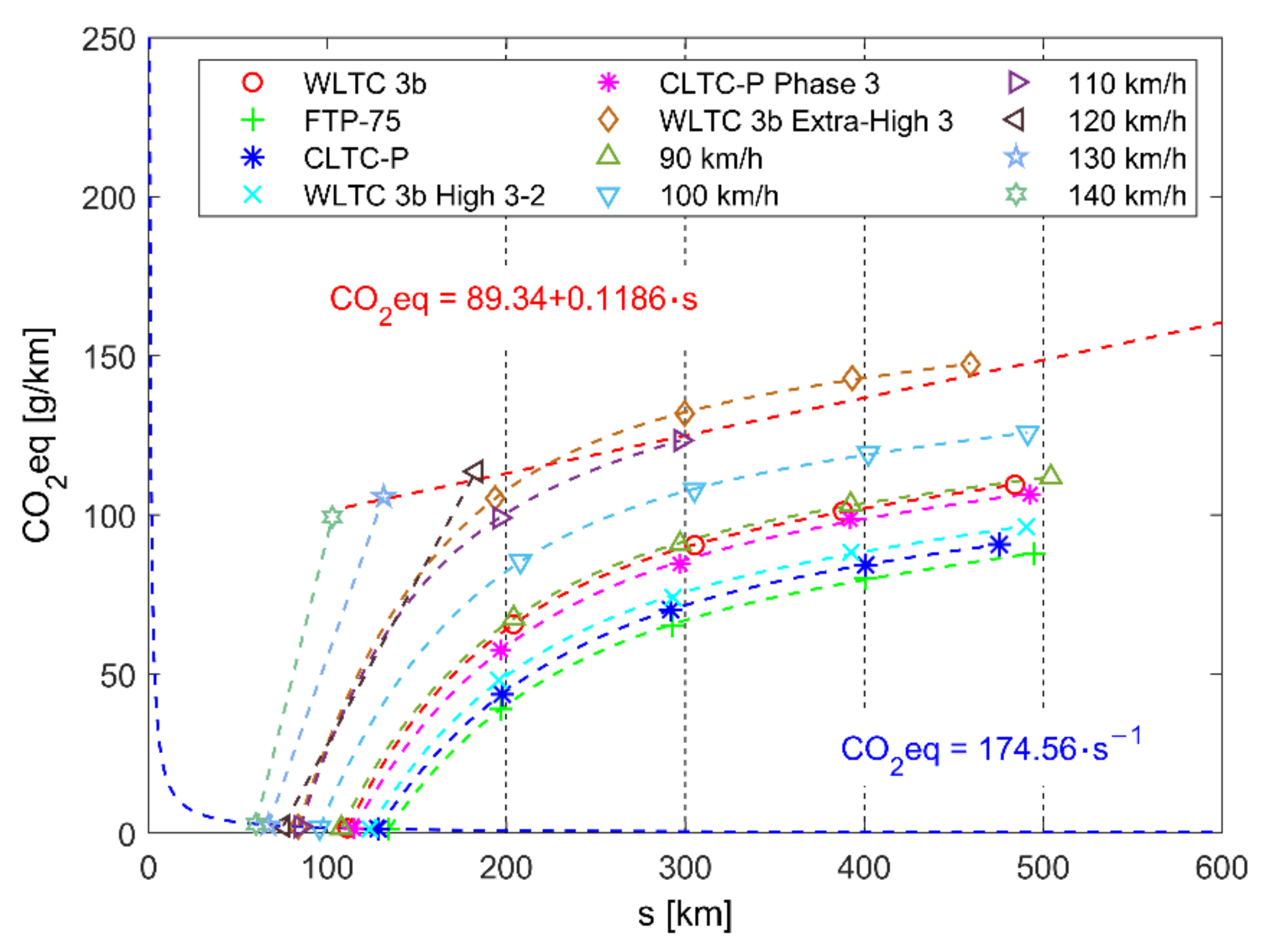
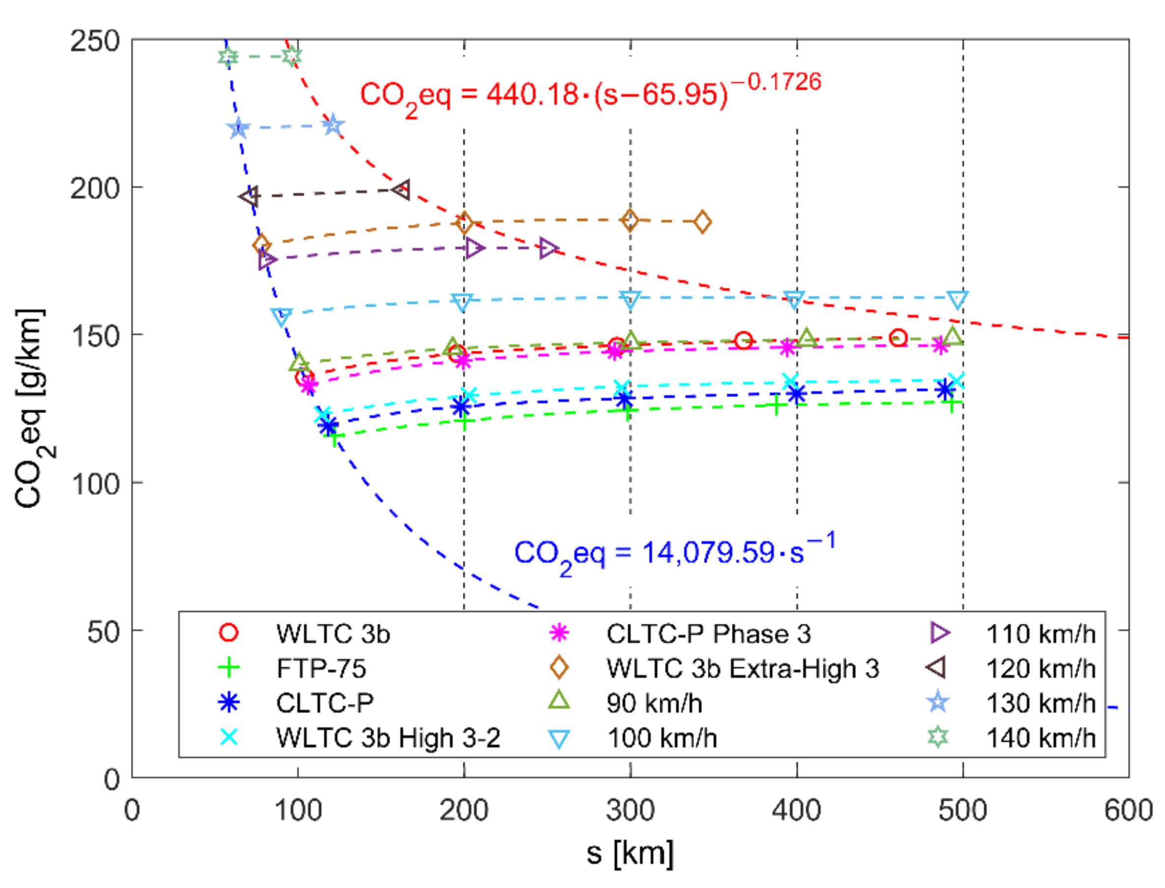
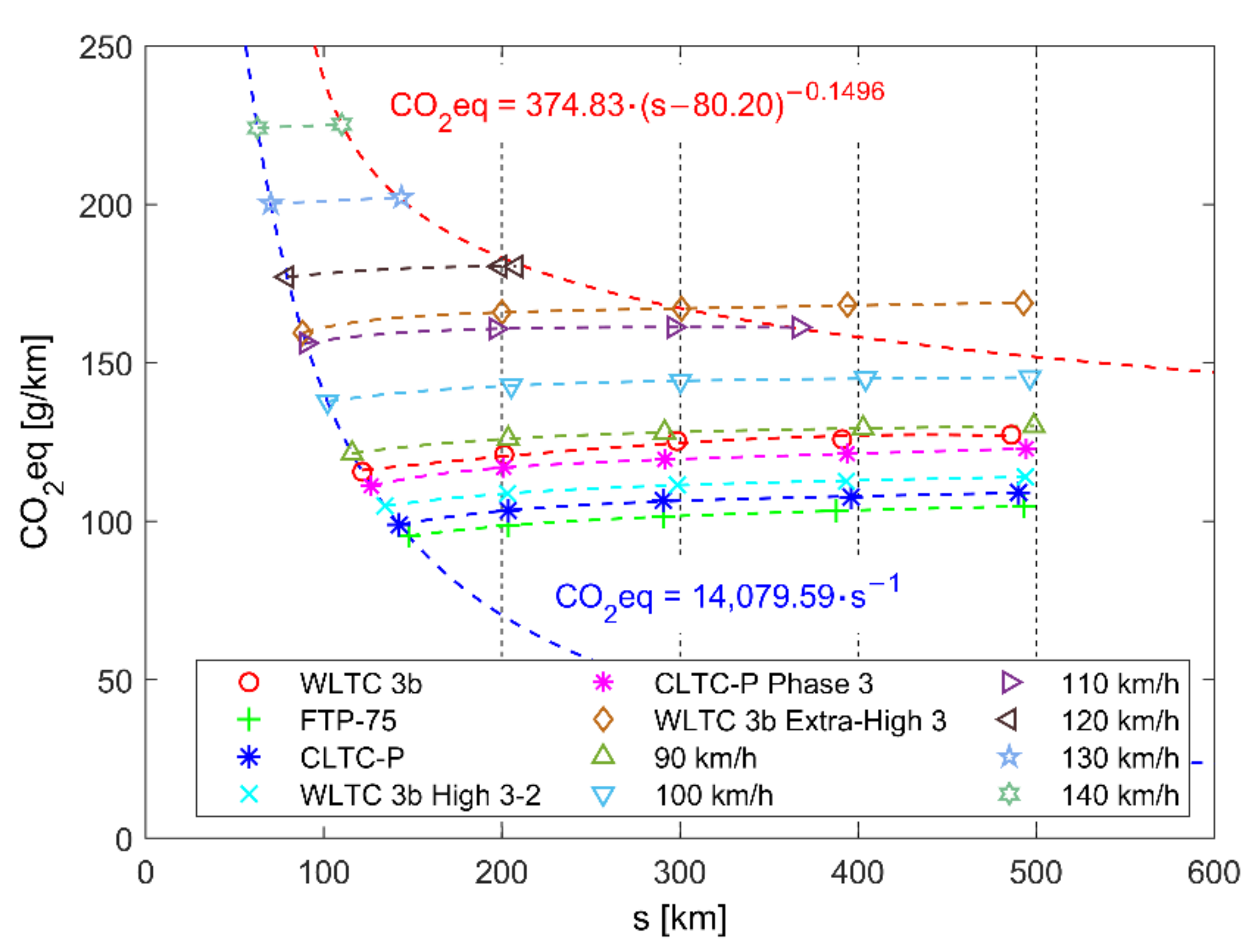
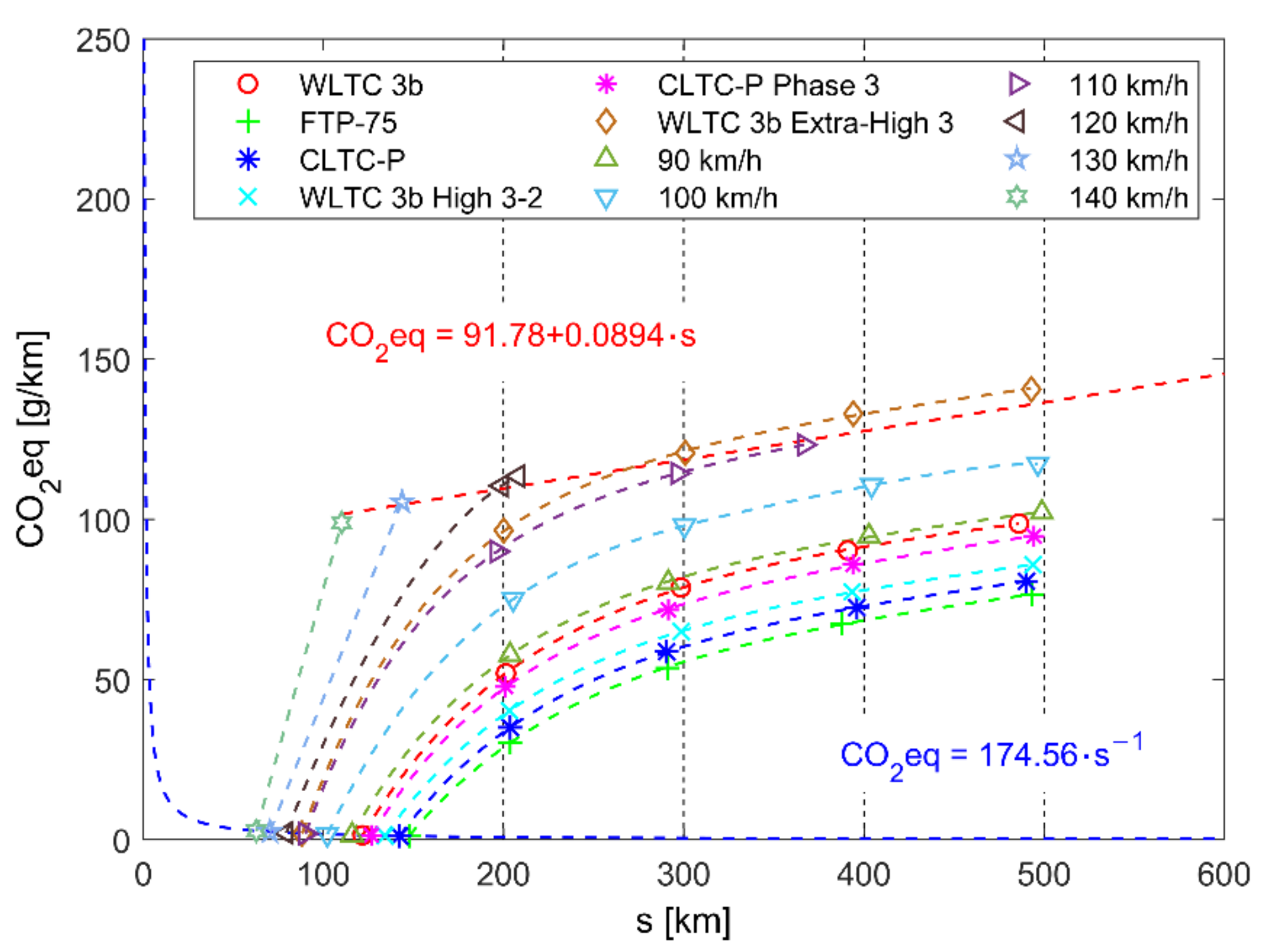
3.6. Combined CO2 Emissions

Combined, road (fuel) and electricity production, CO2eq per 100 km emission values were obtained for four different target range values (200, 300, 400, and 500 km), as well as for BEV mode drive, and for 12 driving cycles. Results for Polish, EU-27, and Swedish average specific emissions from electricity are presented in Figure 13, Figure 14 and Figure 15 respectively. Results for vehicle masses of 1800 kg and 2100 kg are included in Appendix B, Figure A7, Figure A8, Figure A9, Figure A10, Figure A11 and Figure A12. The same markers (for the same drive cycle) are connected making trend lines.
In the case of Polish produced electricity trend lines stay almost flat (Figure 13) indicating that CO2eq emission from electricity, in this use case scenario, almost matches these from gasoline. The CO2eq emission is in the range of 95.3–225.1 g/km. With vehicle mass increasing to 2100 kg (Figure A10, Appendix B) this range increases to 115.7–244.2 g/km. There are also two additional trend lines, with equations describing them. The blue line makes the trend of CO2eq per 100 km emission of BEV mode drive for constant speeds. The red line makes the trend of CO2eq emission per 100 km for EREV drive for maximal range extension in constant speed driving conditions. The area between these two roughly encloses most of the possible CO2eq per 100 km emission area and all CO2eq per 100 km emission area for constant speed drive. With an increase in vehicle speed, CO2eq per 100 km emission rises to high levels, and driving range decreases diminishing EREV utility.
In the case of EU-27 (by average) produced electricity trend lines connecting values of CO2eq per 100 km with increasing range start from a low value (when comparing to results for Polish produced electricity), raise and saturate at some lever (Figure 14). Low initial values indicate a positive influence of lower CO2eq per kWh emission intensity at the EU-27 level, decreasing CO2eq per 100 km emission, both in BEV mode and for lower values of target ranges as EREV. The CO2eq emission is in the range of 31.0–149.6 g/km (a decrease between 67.5% and 33.5% compared to Poland). With vehicle mass increasing to 2100 kg (Figure A11, Appendix B) this range increases to 37.6–160.5 g/km (a decrease between 67.5% and 34.2% compared to Poland). The area between two enclosing trend lines (blue and red) is regular, and the top limit of CO2eg per 100 km stays relatively flat, making almost constant CO2eq per 100 km maximum.
The last case is for Swedish-produced electricity. Trend lines connecting values of CO2eq per 100 km start from very low values (both, when compared to results for Polish produced electricity and EU-27 produced electricity) and raise with diminishing rate as the range increases (Figure 15). Sweden has very low CO2eq per kWh emission intensity, which gives the lowest results of CO2eq per 100 km emission both in BEV mode as well as in the EREV model (when compared to Poland and EU-27 average). The CO2eq emission is in range of 1.2–140.6 g/km (decrease between 98.8% and 37.5% comparing to Poland, and 96.2% and 6.0% comparing to EU-27 average). With vehicle mass increasing to 2100 kg (Figure A12, Appendix B) this range increases to 1.4–147.6 g/km (a decrease between 98.5% and 34.4% compared to Poland, and 95.4% and 1.3% compared to the EU-27 average). The area between two enclosing trend lines (blue and red) is regular, and the top limit of CO2eq per 100 km increases with range.
An important factor is that at the tail end, meaning at high range values (when EREV range is extended much over BEV mode range) the differences in emission of CO2eq per 100 km between Poland, EU-27, and Sweden diminish and are determined by the power demand (in this study determined mostly by driving cycle and mass) and range. For example, for a mass of 1500 kg and a range target of 500 km, the lowest CO2eq per 100 km emission for FTP-75 drive cycle is 104.7, 85.5, and 76.5 g/km (for Poland, EU-27, and Sweden respectively) and the highest is at 168.9, 149.6 and 140.6 g/km (for Poland, EU-27 and Sweden respectively). The results suggest that EREVs may have been under some scrutiny over relatively high CO2eq per 100 km emission when compared to BEVs. Only when EREV range extension over BEV mode range is small to moderate, driving cycle is moderate with its speed and CO2eq per kWh of country or region is low, then CO2eq per 100 km emission can stay at a low level. When these conditions are met EREV provides some flexibility in vehicle range, keeping the negatives of using ICE in check.

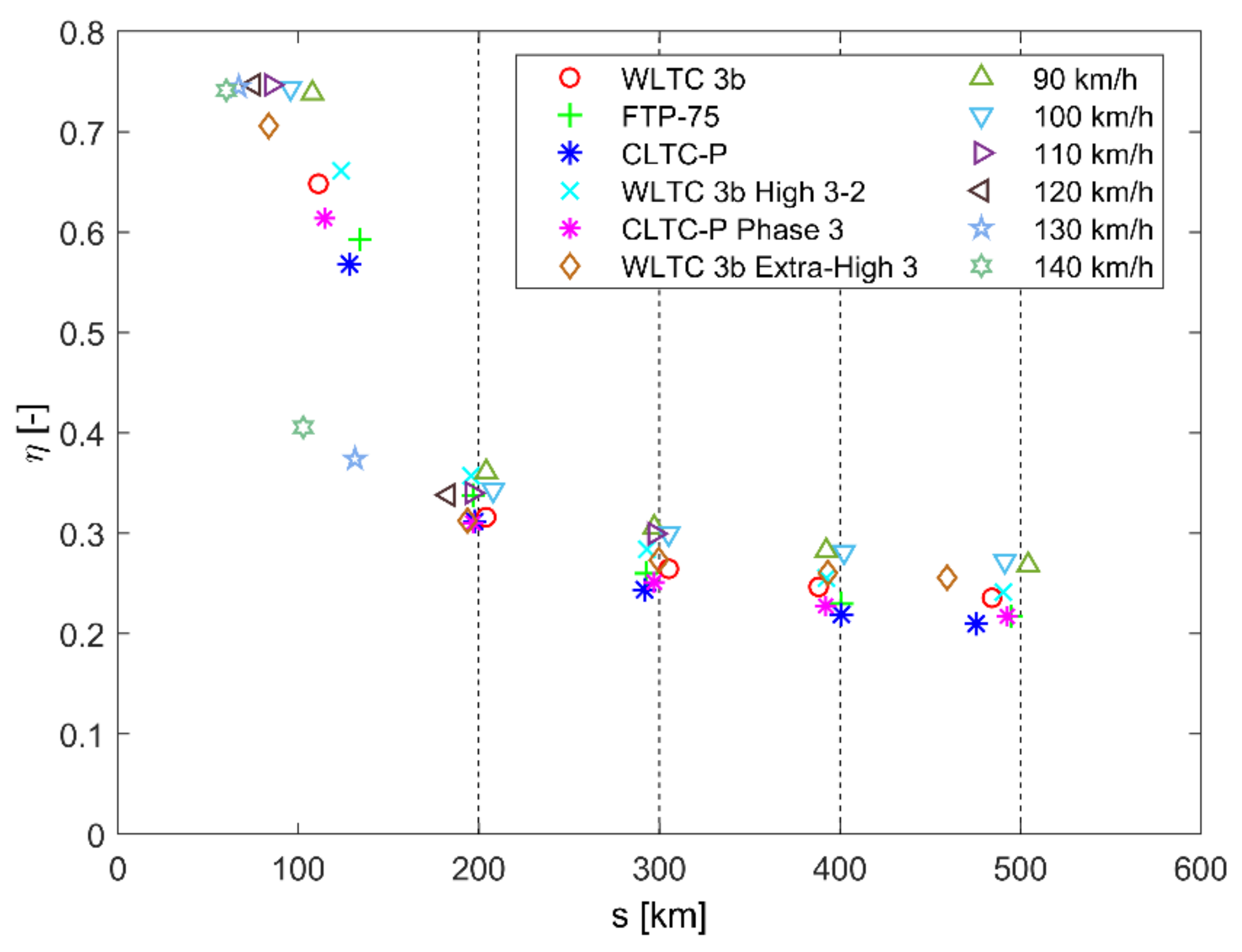
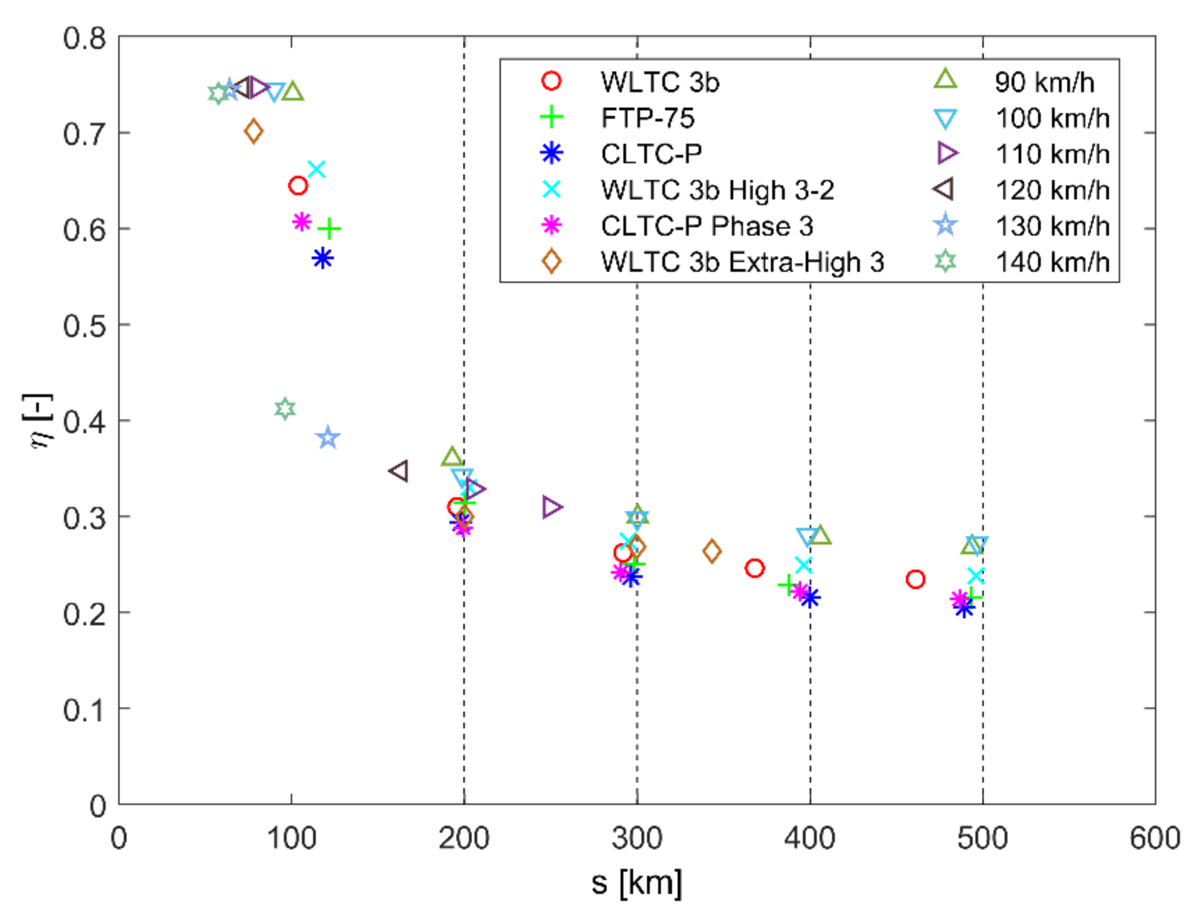
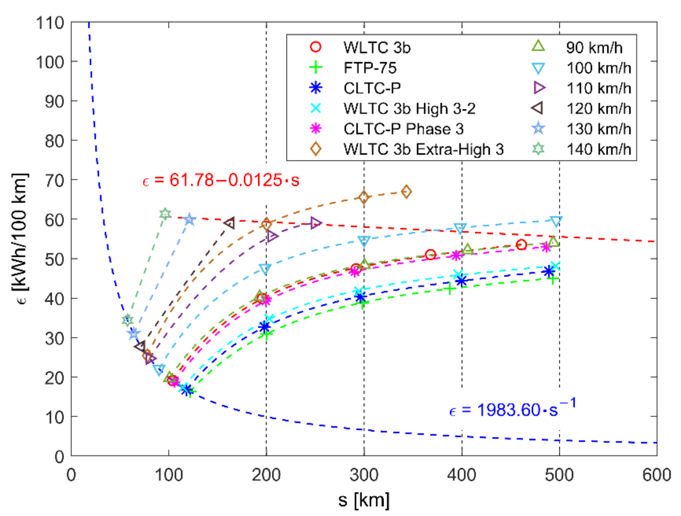
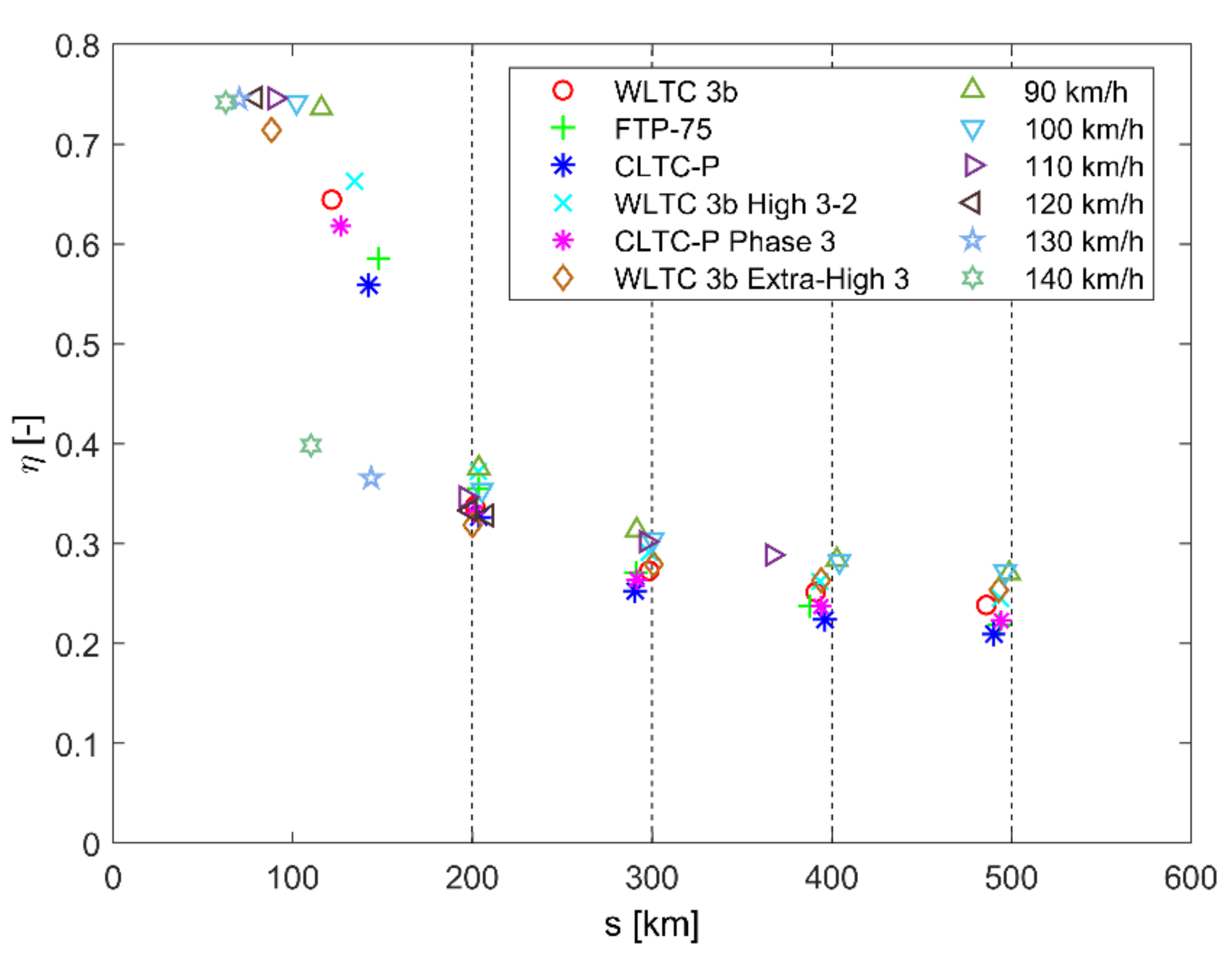
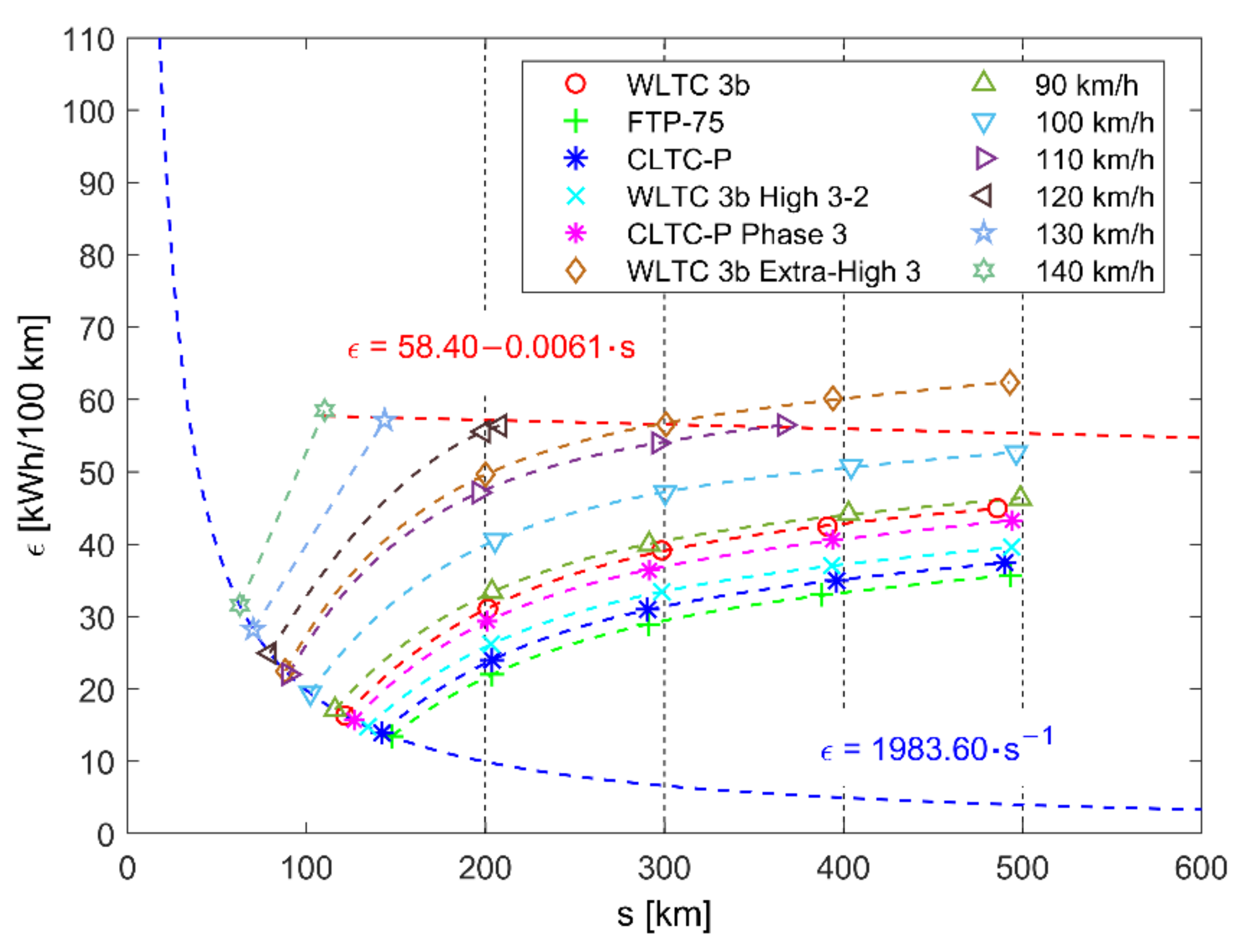
3.7. Powertrain Efficiency and Specific Energy Consumption

The powertrain efficiency is calculated as a ratio of output energy to input energy. Energy values are specified at the end of the drive. The output energy is equal to the work of resistance forces at a driven distance. The input energy is the combined energy content of consumed fuel and electric energy consumed by the charger for vehicle charging. The efficiency results for BEV mode and EREV drive (four EREV range targets) in various drive cycle conditions are shown in Figure 16. These results are for the vehicle mass of 1500 kg. Results for masses of 1800 kg and 2100 kg are presented in Appendix B, Figure A13 and Figure A14.
The efficiency values of the powertrain working in BEV mode are grouped in the range of 55.9–74.7% (56.8–74.7% for 1800 kg and 56.0–74.7% for 2100 kg). For range, extension efficiency drops significantly to the range of 21.0–39.8% (21.0–40.6% for the mass of 1800 kg and 20.6–41.2% for 2100 kg). The highest values of efficiency, regarding cycle type, are for constant speed drive. Driving with constant speed maximizes efficiency, avoiding regenerative braking, which creates higher losses. Of course, regenerative braking is the next best thing since when the driver requires to stop, some of the vehicle’s kinetic energy will be transformed into electricity and go to the battery. Cycles with a lot of starts and stops, such as FTP-75 and CLTC-P, tend to lead to lower efficiency results. From main tree drive cycles in selected order (WLTC 3b, FTP-75 and CLTC-P) average efficiency values when range is extended (vehicle mass of 1500 kg) are 27.5%, 27.1% and 25.3% (comparing to 64.4%, 58.4% and 55.9% in BEV mode). When the mass is increased to 1800 kg average efficiency values when the range is extended are 26.6%, 26.1%, and 24.6%, and when mass is increased to 2100 kg efficiency values decrease further to 26.3%, 25.2%, and 23.8%.
Another measure of efficiency is specific energy consumption in kilowatt-hours per 100 km. Here the input energy is divided by the traveled distance in hundreds of kilometers. The specific energy consumption results for BEV mode and EREV drive (four EREV range targets) in various drive cycle conditions are shown in Figure 17. These results are for a vehicle mass of 1500 kg. Results for masses of 1800 kg and 2100 kg are presented in Appendix B, Figure A15 and Figure A16.
Specific energy consumption is often used to describe BEVs. Points of BEV mode results are placed roughly on a blue dashed trend line, with an equation describing the trend. These values are in the range of 13.4–31.6 kWh/100 km (14.8–33.0 kWh/100 km for the mass of 1800 kg and 16.3–34.4 kWh/100 km for 2100 kg). Tree main drive cycles (WLTC 3b, FTP-75, and CLTC-P) produce average specific energy consumption, when range extending (vehicle mass of 1500 kg) of 39.4 kWh/100 km, 29.9 kWh/100 km, and 31.8 kWh/100 km (comparing to 16.3 kWh/100 km, 13.4 kWh/100 km and 13.9 kWh/100 km in BEV mode). When the mass is increased to 1800 kg average specific energy consumption values increase to 44.3 kWh/100 km, 34.5 kWh/100 km, and 36.3 kWh/100 km, and when mass is increased to 2100 kg average specific energy consumption values increase further to 48.0 kWh/100 km, 39.3 kWh/100 km, and 41.1 kWh/100 km. Here the cycles with less power demand generate the lowest specific energy consumption, with FTP-75 leading in this regard.

3.8. Study Limitations

This study is based to a large extent on the results of multiple runs of computer simulation. Computer models cannot perfectly describe the underlying physical phenomena by mathematical models. There is always some approximation to the model and set of assumptions to reduce complex models to a simpler form. Another factor is the model output (result) sensitivity to the input (input data).
The main study limitation is the lack of result validation in real objects—running EREV with REX controlled by the proposed strategy, tested in drive cycle conditions. The plan for future research is the proposal to validate main powertrain components in laboratory test conditions and road conditions. Some of the simulation result validation requires careful preparation, multiple tests, and validation of many test points. Some of the research shown in this study have the simulation results of component validated, like the REX BFSC map, but there are changes accommodating the REX model to the vehicle model.
Another limiting factor is model simplification in regard to omitting certain physic phenomena. The next step in EREV model development is to broaden the scope of the model, to include the thermal modeling of key powertrain components, starting with the battery. The battery temperature can be a limiting factor when delivering power to the motor and its performance influences the performance of the whole powertrain.
The control strategy operation is set so that battery SOC drops linearly over traveled distance. This relation between battery SOC and s should be further investigated. For example, change in the control strategy could provide a faster drop of battery SOC at high battery SOC levels and a slower drop of battery SOC at low levels of battery SOC. Such an approach can lead to keeping battery voltage at moderate levels for more time, which could be beneficial in terms of battery efficiency or battery health.

4. Conclusions

This study investigated the EREV performance in the real road conditions defined by WLTC 3b, FTP-75, and CLTC-P drive cycles plus three cycle fragments. Six variants of constant speed drive between 90 km/h and 140 km/h were also included. The analysis was carried out based on the simulation performed in Matlab-Simulink®. It included four different drive range targets of the vehicle (200, 300, 400, and 500 km), three vehicle masses (1500, 1800, and 2100 kg), and three cases of the electricity mix (Polish, EU-27, and Swedish). The main findings from the study are as follows:
  • EREV model based on component modeling is presented and simulation runs were successful.
  • The REX control strategy was presented and implemented, with the goal of governing REX operation periods and adapting to the required range target.
  • BEV mode ranges were calculated, showing a potential need for extending the BEV range.
  • The REX control strategy can cope with various driving conditions—six drive cycles and six constant speeds have been tested, including WLTC 3b, FTP-75, and CLTC-P, for three vehicle masses. Comparisons of the actual ranges obtained to range targets showed good performance of the control strategy, with an average difference between −0.51% and −1.34% for three vehicle mass variants.
  • The REX control strategy ensures a linear drop of SOC over traveled distance. Further research on this relation is advised, due to the battery efficiency and battery voltage over drive time potential improvements.
  • For some high range targets and more demanding drive conditions REX utilization was close to 100%, showing limitations of range extension for REX in certain power settings.
  • The REX engagement instances and running time periods were classified. The REX average run time instance, as well as the majority of instance run times were well above the set “soft minimum” of 120 s. The distribution of binned run time instances showed for WLTC 3b is much broader in time spectrum, with a more uniform value count, compared to FTP-75 and CLTC-P.
  • Fuel consumption was calculated. The CO2eq emission contribution from the fuel is independent of the country or the region in which EREV is operated. For Sweden, this results in a vast increase of EREV CO2eq emission over the BEV mode operation. This cautions moderation in setting range extension targets over the BEV mode range.
  • For countries with high CO2eq emission from grid electricity, like the presented case of Poland, EREV CO2eq emission proves to be staying at high levels, no matter what range target was selected.
  • The results show detailed relations between EREV CO2eq emission and vehicle range. Areas of possible emission are pointed out, showing the broad range of possible values. This further emphasized need for treating EVER accordingly to local conditions, especially to CO2 transport emission policy.
  • EREV powertrain efficiency stays within the range of 21.0–41.2% for tested cases. These are respectable values but fall short of the BEV mode efficiency range of 55.9–74.7%. Yet still, EREV has the capability of BEV mode drive, having the possibility of zero tailpipe emission and range extension when needed.

Author Contributions

Conceptualization, P.K.; methodology, P.K., A.K. and J.L.; software, P.K.; validation, P.K., A.K. and J.L.; formal analysis, P.K.; investigation, P.K., J.L.; resources, A.K.; data curation, P.K.; writing—original draft preparation, P.K.; writing—review and editing, A.K. and J.L.; visualization, P.K., A.K.; supervision, P.K.; project administration, A.K.; funding acquisition, P.K. All authors have read and agreed to the published version of the manuscript.

Funding

The APC was funded by Warsaw University of Technology, Board of Mechanical Engineering internal grant supporting scientific endeavors in mechanical engineering: “Research of parameters of Extended-Range Electric Vehicle”.

Institutional Review Board Statement

Not applicable.

Informed Consent Statement

Not applicable.

Data Availability Statement

Not applicable.

Conflicts of Interest

The authors declare no conflict of interest.

Abbreviations

BATElectrochemical battery pack
BEVBattery Electric Vehicle
BSFCBrake Specific Fuel Consumption
CLTCChina Light-Duty Vehicle Test Cycle
CO2eqCarbon Dioxide Equivalent
CSControl Strategy
DCDriving Cycle
ECUElectronic Control Unit
EMElectric Motor
EREVExtended-Range Electric Vehicle
EVElectric Vehicle
FTP-75Federal Test Procedure
GElectric generator
H.High
HEVHybrid Electric Vehicle
ICEInternal Combustion Engine
LAVLeisure Activity Vehicle
LPGLiquefied Petroleum Gas
PIProportional-Integral
PMSMPermanent Magnet Synchronous Motor
PSPower summing node
REXRange Extender
SOCState of Charge
VEVehicle and driveline
WRoad wheels
WLTC 3bWorldwide Harmonized Light-duty Test Cycle Class 3b
ZDACZero d-axis current control strategy

Appendix A

Additional sets of simulation results.
Table A1. Difference between range target and traveled range at 15% SOC. Bolded values indicate cases when the range target cannot be obtained. Vehicle mass is 1800 kg. The average percent difference (excluding data when range cannot be obtained) is −1.00%, with a standard deviation of 1.83%.
Range Target200 km300 km400 km500 km
WLTC 3b204.02
(2.01)
305.23
(1.74)
388.20
(−2.95)
484.25
(−3.15)
FTP-75196.88
(−1.56)
292.71
(−2.43)
400.90
(0.22)
494.80
(−1.04)
CLTC-P197.66
(−1.17)
291.82
(−2.73)
400.80
(0.20)
475.46
(−4.91)
WLTC 3b High 3-2195.81
(−2.09)
293.12
(−2.29)
392.60
(−1.85)
490.61
(−1.88)
CLTC-P Phase 3196.78
(−1.61)
297.13
(−0.96)
392.11
(−1.97)
492.75
(−1.45)
WLTC 3b Extra-H. 3193.68
(−3.16)
299.62
(−0.13)
393.33
(−1.67)
459.34
(−8.13)
90 km/h204.14
(2.07)
297.12
(−0.96)
392.45
(−1.89)
504.31
(0.86)
100 km/h207.94
(3.97)
305.13
(1.71)
402.32
(0.58)
491.38
(−1.73)
110 km/h196.18
(−1.91)
297.34
(−0.89)
297.37
(−25.66)
297.39
(−40.52)
120 km/h183.02
(−8.49)
183.02
(−38.99)
183.02
(−54.24)
183.02
(−63.40)
130 km/h131.43
(−34.29)
131.44
(−56.19)
131.46
(−67.14)
131.47
(−73.71)
140 km/h102.76
(−48.62)
102.76
(−65.75)
102.76
(−74.31)
102.76
(−79.45)
Unitkm
(%)
km
(%)
km
(%)
km
(%)
Table A2. Difference between range target and traveled range at 15% SOC. Bolded values indicate cases when the range target cannot be obtained. Vehicle mass is 2100 kg. The average percent difference (excluding data when range cannot be obtained) is −1.34%, with a standard deviation of 2.18%.
Range Target200 km300 km400 km500 km
WLTC 3b195.75
(−2.12)
291.87
(−2.71)
368.06
(−7.98)
461.17
(−7.77)
FTP-75200.18
(0.09)
298.09
(−0.64)
388.09
(−2.98)
493.18
(−1.37)
CLTC-P198.01
(−0.99)
296.35
(−1.22)
399.99
(−0.00)
489.46
(−2.11)
WLTC 3b High 3-2202.74
(1.37)
294.72
(−1.76)
396.36
(−0.91)
496.21
(−0.76)
CLTC-P Phase 3199.38
(−0.31)
290.67
(−3.11)
394.26
(−1.44)
486.56
(−2.69)
WLTC 3b Extra-H. 3200.19
(0.09)
299.75
(−0.08)
343.32
(−14.17)
343.36
(−31.33)
90 km/h193.00
(−3.50)
300.34
(0.11)
406.00
(1.50)
493.80
(−1.24)
100 km/h198.68
(−0.66)
299.97
(−0.01)
398.45
(−0.39)
496.85
(−0.63)
110 km/h205.21
(2.61)
249.63
(−16.79)
249.66
(−37.59)
249.68
(−50.06)
120 km/h163.28
(−18.36)
163.28
(−45.57)
163.28
(−59.18)
163.28
(−67.34)
130 km/h121.03
(−39.48)
121.05
(−59.65)
121.06
(−69.73)
121.07
(−75.79)
140 km/h96.24
(−51.88)
96.24
(−67.92)
96.24
(−75.94)
96.24
(−80.75)
Unitkm
(%)
km
(%)
km
(%)
km
(%)
Table A3. Average REX single instance running time and the total number of engagements (in parentheses) for four range targets in WLTC 3b, FTP-75, and CLTC-P drive cycles. Vehicle mass is 1800 kg.
Range Target200 km300 km400 km500 km
WLTC 3b266
(13)
401
(18)
354
(29)
375
(37)
FTP-75195
(10)
196
(25)
188
(44)
183
(61)
CLTC-P220
(10)
211
(25)
243
(36)
233
(48)
Units
(-)
s
(-)
s
(-)
s
(-)
Table A4. Average REX single instance running time and the total number of engagements (in parentheses) for four range targets in WLTC 3b, FTP-75, and CLTC-P drive cycles. Vehicle mass is 2100 kg.
Range Target200 km300 km400 km500 km
WLTC 3b228
(16)
356
(21)
393
(27)
422
(34)
FTP-75219
(12)
199
(30)
192
(47)
182
(69)
CLTC-P256
(11)
261
(24)
235
(42)
214
(61)
Units
(-)
s
(-)
s
(-)
s
(-)
Table A5. REX utilization measures % of total driving time when REX is enabled. Bolded values indicate that REX is engaged once and working constantly, and a range target cannot be obtained. Vehicle mass equals to 1800 kg.
Range Target200 km300 km400 km500 km
WLTC 3b21.5630.0433.7836.84
FTP-759.3415.8519.4821.35
CLTC-P8.8014.3617.4518.84
WLTC 3b High 3-219.1630.1135.8638.99
CLTC-P Phase 320.6030.6835.5338.55
WLTC 3b Extra-H. 369.4387.3196.0599.87
90 km/h43.7059.0367.2072.86
100 km/h61.7278.5187.1992.13
110 km/h79.2899.9399.9499.94
120 km/h99.8799.8799.8799.87
130 km/h99.8199.8299.8399.84
140 km/h99.7499.7499.7499.74
Unit%%%%
Table A6. REX utilization measures % of total driving time when REX is enabled. Bolded values indicate that REX is engaged once and working constantly, and a range target cannot be obtained. Vehicle mass equals to 2100 kg.
Range Target200 km300 km400 km500 km
WLTC 3b23.3932.6637.0240.03
FTP-7512.4918.8121.9724.00
CLTC-P11.2816.8419.7121.37
WLTC 3b High 3-224.5234.3940.0843.14
CLTC-P Phase 325.6834.7639.9142.78
WLTC 3b Extra-H. 377.6494.8399.8299.84
90 km/h47.3165.7874.4378.80
100 km/h66.2584.7993.7899.21
110 km/h89.6499.9199.9199.92
120 km/h99.8499.8499.8499.84
130 km/h99.7699.7899.7999.80
140 km/h99.6899.6899.6899.68
Unit%%%%
Table A7. Fuel consumption in EREV mode for WLTC 3b High 3-2.
Range Target200 km300 km400 km500 km
Mass = 1500 kg1.84
(203.34)
3.00
(298.60)
3.58
(393.62)
3.98
(493.87)
Mass = 1800 kg2.19
(195.81)
3.42
(293.12)
4.09
(392.60)
4.47
(490.61)
Mass = 2100 kg2.80
(202.74)
3.92
(294.72)
4.60
(396.36)
4.94
(496.21)
Unitdm3/100 km
(km)
dm3/100 km
(km)
dm3/100 km
(km)
dm3/100 km
(km)
Table A8. Fuel consumption in EREV mode for CLTC-P Phase 3.
Range Target200 km300 km400 km500 km
Mass = 1500 kg2.18
(201.05)
3.32
(291.58)
3.98
(393.86)
4.40
(494.27)
Mass = 1800 kg2.64
(196.78)
3.92
(297.13)
4.57
(392.11)
4.95
(492.75)
Mass = 2100 kg3.29
(199.38)
4.46
(290.67)
5.12
(394.26)
5.47
(486.56)
Unitdm3/100 km
(km)
dm3/100 km
(km)
dm3/100 km
km
dm3/100 km
(km)
Table A9. Fuel consumption in EREV mode for WLTC 3b Extra-High 3.
Range Target200 km300 km400 km500 km
Mass = 1500 kg4.45
(200.20)
5.60
(300.86)
6.18
(394.15)
6.53
(492.86)
Mass = 1800 kg4.86
(193.68)
6.11
(299.62)
6.64
(393.33)
6.84
(459.34)
Mass = 2100 kg5.47
(200.19)
6.60
(299.75)
6.85
(343.32)
6.85
(343.36)
Unitdm3/100 km
(km)
dm3/100 km
(km)
dm3/100 km
(km)
dm3/100 km
(km)
Table A10. Fuel consumption in EREV mode for constant speed drive at 110 km/h.
Range Target200 km300 km400 km500 km
Mass = 1500 kg2.65
(203.63)
3.71
(291.44)
4.40
(402.86)
4.74
(498.81)
Mass = 1800 kg3.11
(204.14)
4.20
(297.12)
4.79
(392.45)
5.19
(504.31)
Mass = 2100 kg3.37
(193.00)
4.68
(300.34)
5.29
(406.00)
5.60
(493.80)
Unitdm3/100 km
(km)
dm3/100 km
(km)
dm3/100 km
(km)
dm3/100 km
(km)
Table A11. Fuel consumption in EREV mode for constant speed drive at 100 km/h.
Range Target200 km300 km400 km500 km
Mass = 1500 kg3.46
(205.38)
4.54
(300.40)
5.13
(404.28)
5.45
(496.52)
Mass = 1800 kg3.94
(207.94)
5.00
(305.13)
5.54
(402.32)
5.84
(491.38)
Mass = 2100 kg4.22
(198.68)
5.38
(299.97)
5.93
(398.45)
6.25
(496.85)
Unitdm3/100 km
(km)
dm3/100 km
(km)
dm3/100 km
(km)
dm3/100 km
(km)
Table A12. Fuel consumption in EREV mode for constant speed drive at 110 km/h.
Range Target200 km300 km400 km500 km
Mass = 1500 kg4.15
(196.53)
5.30
(296.55)
5.72
(366.85)
5.72
(366.87)
Mass = 1800 kg4.57
(196.18)
5.72
(297.34)
5.72
(297.37)
5.72
(297.39)
Mass = 2100 kg5.16
(205.21)
5.72
(249.63)
5.72
(249.66)
5.72
(249.68)
Unitdm3/100 km
(km)
dm3/100 km
(km)
dm3/100 km
(km)
dm3/100 km
(km)
Table A13. Fuel consumption in EREV mode for constant speed drive at 120 km/h.
Range Target200 km300 km400 km500 km
Mass = 1500 kg5.11
(198.90)
5.25
(207.98)
5.25
(207.98)
5.25
(207.98)
Mass = 1800 kg5.25
(183.02)
5.25
(183.02)
5.25
(183.02)
5.25
(183.02)
Mass = 2100 kg5.25
(163.28)
5.25
(163.28)
5.25
(163.28)
5.25
(163.28)
Unitdm3/100 km
(km)
dm3/100 km
(km)
dm3/100 km
(km)
dm3/100 km
(km)
Table A14. Fuel consumption in EREV mode for constant speed drive at 130 km/h.
Range Target200 km300 km400 km500 km
Mass = 1500 kg4.85
(143.69)
4.85
(143.71)
4.85
(143.72)
4.85
(143.72)
Mass = 1800 kg4.86
(131.43)
4.86
(131.44)
4.86
(131.46)
4.86
(131.47)
Mass = 2100 kg4.87
(121.03)
4.87
(121.05)
4.87
(121.06)
4.87
(121.07)
Unitdm3/100 km
(km)
dm3/100 km
(km)
dm3/100 km
(km)
dm3/100 km
(km)
Table A15. Fuel consumption in EREV mode for constant speed drive at 140 km/h.
Range Target200 km300 km400 km500 km
Mass = 1500 kg4.54
(110.20)
4.54
(110.20)
4.54
(110.20)
4.54
(110.20)
Mass = 1800 kg4.55
(102.76)
4.55
(102.76)
4.55
(102.76)
4.55
(102.76)
Mass = 2100 kg4.56
(96.24)
4.56
(96.24)
4.56
(96.24)
4.56
(96.24)
Unitdm3/100 km
(km)
dm3/100 km
(km)
dm3/100 km
(km)
dm3/100 km
(km)

Appendix B

Additional figures presenting simulation results.
Figure A1. REX engagement instances binned by engagement time for WLTC 3b and vehicle mass of 1800 kg.
Energies 15 04187 g0a1
Figure A2. REX engagement instances binned by engagement time for FTP-75 and vehicle mass of 1800 kg.
Energies 15 04187 g0a2
Figure A3. REX engagement instances binned by engagement time for CLTC-P and vehicle mass of 1800 kg.
Energies 15 04187 g0a3
Figure A4. REX engagement instances binned by engagement time for WLTC 3b and vehicle mass of 2100 kg.
Energies 15 04187 g0a4
Figure A5. REX engagement instances binned by engagement time for FTP-75 and vehicle mass of 2100 kg.
Energies 15 04187 g0a5
Figure A6. REX engagement instances binned by engagement time for CLTC-P and vehicle mass of 2100 kg.
Energies 15 04187 g0a6
Figure A7. Combined CO2eq emission, due to EREV operation and electricity production (Poland), in various driving conditions. Note that the blue approximation line (BEV mode) and the red approximation line (maximal range) are obtained for constant speed driving results from the range of 90–140 km/h. Vehicle mass is equal to 1800 kg.
Energies 15 04187 g0a7
Figure A8. Combined CO2eq emission, due to EREV operation and electricity production (EU-27), in various driving conditions. Note that the blue approximation line (BEV mode) and the red approximation line (maximal range) are obtained for constant speed driving results from the range of 90–140 km/h. Vehicle mass is equal to 1800 kg.
Energies 15 04187 g0a8
Figure A9. Combined CO2eq emission, due to EREV operation and electricity production (Sweden), in various driving conditions. Note that the blue approximation line (BEV mode) and the red approximation line (maximal range) are obtained for constant speed driving results from the range of 90–140 km/h. Vehicle mass is equal to 1800 kg.
Energies 15 04187 g0a9
Figure A10. Combined CO2eq emission, due to EREV operation and electricity production (Poland), in various driving conditions. Note that the blue approximation line (BEV mode) and the red approximation line (maximal range) are obtained for constant speed driving results from the range of 90–140 km/h. Vehicle mass is equal to 2100 kg.
Energies 15 04187 g0a10
Figure A11. Combined CO2eq emission, due to EREV operation and electricity production (EU-27), in various driving conditions. Note that the blue approximation line (BEV mode) and the red approximation line (maximal range) are obtained for constant speed driving results from the range of 90–140 km/h. Vehicle mass is equal to 2100 kg.
Energies 15 04187 g0a11
Figure A12. Combined CO2eq emission, due to EREV operation and electricity production (Sweden), in various driving conditions. Note that the blue approximation line (BEV mode) and the red approximation line (maximal range) are obtained for constant speed driving results from the range of 90–140 km/h. Vehicle mass is equal to 2100 kg.
Energies 15 04187 g0a12
Figure A13. Efficiency results for BEV mode and EREV drive (four EREV range targets indicated with dashed vertical lines) in various drive cycle conditions. Vehicle mass is equal to 1800 kg.
Energies 15 04187 g0a13
Figure A14. Efficiency results for BEV mode and EREV drive (four EREV range targets indicated with dashed vertical lines) in various drive cycle conditions. Vehicle mass is equal to 2100 kg.
Energies 15 04187 g0a14
Figure A15. Specific energy consumption results for BEV mode and EREV drive (four EREV range targets indicated with dashed vertical lines) in various drive cycle conditions. Vehicle mass is equal to 1800 kg.
Energies 15 04187 g0a15
Figure A16. Specific energy consumption results for BEV mode and EREV drive (four EREV range targets indicated with dashed vertical lines) in various drive cycle conditions. Vehicle mass is equal to 2100 kg.
Energies 15 04187 g0a16

References

  1. Gössling, S.; Cohen, S.A.; Higham, J.E.S.; Peeters, P.M.; Eijgelaar, E. Desirable transport futures. Transp. Res. Part D Transp. Environ. 2018, 61, 301–309. [Google Scholar] [CrossRef]
  2. Duell, M.; Gardner, L.M.; Waller, S.T. Policy implications of incorporating distance constrained electric vehicles into the traffic network design problem. Transp. Lett. 2018, 10, 144–158. [Google Scholar] [CrossRef]
  3. Wilberforce, T.; El-Hassan, Z.; Khatib, F.N.; Al Makky, A.; Baroutaji, A.; Carton, J.G.; Olabi, A.G. Developments of electric cars and fuel cell hydrogen electric cars. Int. J. Hydogen Energy 2017, 42, 25695–25734. [Google Scholar] [CrossRef] [Green Version]
  4. Szumanowski, A.; Chang, Y.; Liu, Z.; Krawczyk, P. Hybrid powertrain efficiency improvement by using electromagnetically controlled double-clutch transmission. Int. J. Veh. Des. 2018, 76, 1–19. [Google Scholar] [CrossRef]
  5. Requia, W.J.; Mohamed, M.; Higgins, C.D.; Arain, A.; Ferguson, M. How clean are electric vehicles? Evidence-based review of the effects of electric mobility on air pollutants, greenhouse gas emissions and human health. Atmos. Environ. 2018, 185, 64–77. [Google Scholar] [CrossRef]
  6. Reiter, M.S.; Kockelman, K.M. Emissions and exposure costs of electric versus conventional vehicles: A case study in Texas. Int. J. Sustain. Transp. 2017, 11, 486–492. [Google Scholar] [CrossRef]
  7. Habib, S.; Khan, M.M.; Abbas, F.; Sang, L.; Shahid, M.U.; Tang, H. A comprehensive study of implemented international standards, technical challenges, impacts and prospects for electric vehicles. IEEE Access. 2018, 6, 13866–13890. [Google Scholar] [CrossRef]
  8. Chłopek, Z.; Lasocki, J.; Wójcik, P.; Badyda, A.J. Experimental investigation and comparison of energy consumption of electric and conventional vehicles due to the driving pattern. Int. J. Green Energy 2018, 15, 773–779. [Google Scholar] [CrossRef]
  9. Sutcu, M. Effects of total cost of ownership on automobile purchasing decisions. Transp. Lett. 2018, 12, 1–7. [Google Scholar] [CrossRef]
  10. Ehsani, M.; Gao, Y.; Longo, S.; Ebrahimi, K. Modern Electric, Hybrid Electric, and Fuel Cell Vehicles; CRC Press: Boca Raton, FL, USA, 2018; ISBN 9781138330498. [Google Scholar]
  11. Kopczyński, A.; Piórkowski, P.; Roszczyk, P. Parameters selection of extended-range electric vehicle powered from supercapacitor pack based on laboratory and simulation tests. IOP Conf. Ser. Mater. Sci. Eng. 2018, 421, 022016. [Google Scholar] [CrossRef]
  12. Vatanparvar, K.; Faezi, S.; Burago, I.; Levorato, M.; Al Faruque, M.A. Extended range electric vehicle with driving behavior estimation in energy management. IEEE Trans. Smart Grid 2018, 10, 2959–2968. [Google Scholar] [CrossRef]
  13. Yao, M.; Zhu, B.; Zhang, N. Adaptive real-time optimal control for energy management strategy of extended range electric vehicle. Energy Convers. Manag. 2021, 234, 113874. [Google Scholar] [CrossRef]
  14. Kalia, A.V.; Fabien, B.C. On Implementing Optimal Energy Management for EREV Using Distance Constrained Adaptive Real-Time Dynamic Programming. Electronics 2020, 9, 228. [Google Scholar] [CrossRef] [Green Version]
  15. Zhu, D.; Pritchard, E.; Dadam, S.R.; Kumar, V.; Xu, Y. Optimization of rule-based energy management strategies for hybrid vehicles using dynamic programming. Combust. Engines 2021, 184, 3–10. [Google Scholar] [CrossRef]
  16. Xiao, B.; Ruan, J.; Yang, W.; Walker, P.D.; Zhang, N. A review of pivotal energy management strategies for extended range electric vehicles. Renew. Sustain. Energy Rev. 2021, 149, 111194. [Google Scholar] [CrossRef]
  17. Basma, H.; Mansour, C.; Halaby, H.; Baz Radwan, A. Methodology to Design an Optimal Rule-Based Energy Management Strategy Using Energetic Macroscopic Representation: Case of Plug-In Series Hybrid Electric Vehicle. Adv. Automob. Eng. 2018, 7, 188. [Google Scholar] [CrossRef]
  18. Salmasi, F.R. Control strategies for hybrid electric vehicles: Evolution, classification, comparison, and future trends. IEEE Trans. Veh. Technol. 2007, 56, 2393–2404. [Google Scholar] [CrossRef]
  19. Hou, C.; Ouyang, M.; Xu, L.; Wang, H. Approximate Pontryagin’s minimum principle applied to the energy management of plug-in hybrid electric vehicles. Appl. Energy 2014, 115, 174–189. [Google Scholar] [CrossRef]
  20. Huang, Y.; Wang, H.; Khajepour, A.; Li, B.; Ji, J.; Zhao, K.; Hu, C. A review of power management strategies and component sizing methods for hybrid vehicles. Renew. Sustain. Energy Rev. 2018, 96, 132–144. [Google Scholar] [CrossRef]
  21. Huang, Y.; Wang, H.; Khajepour, A.; He, H.; Ji, J. Model predictive control power management strategies for HEVs: A review. J. Power Sources 2017, 341, 91–106. [Google Scholar] [CrossRef]
  22. Xing, Y.; Ma, E.W.M.; Tsui, K.L.; Pecht, M. Battery management systems in electric and hybrid vehicles. Energies 2011, 4, 1840–1857. [Google Scholar] [CrossRef]
  23. Peng, J.; He, H.; Xiong, R. Rule based energy management strategy for a series-parallel plug-in hybrid electric bus optimized by dynamic programming. Appl. Energy 2017, 185, 1633–1643. [Google Scholar] [CrossRef]
  24. Geng, B.; Mills, J.K.; Sun, D. Energy management control of mictroturbine-powered plug-in hybrid electric vehicles using the telemetry equivalent consumption minimization strategy. IEEE Trans. Veh. Technol. 2011, 60, 4238–4248. [Google Scholar] [CrossRef]
  25. Lü, X.; Wu, Y.; Lian, J.; Zhang, Y.; Chen, C.; Wang, P.; Meng, L. Energy management of hybrid electric vehicles: A review of energy optimization of fuel cell hybrid power system based on genetic algorithm. Energy Convers. Manag. 2020, 205, 112474. [Google Scholar] [CrossRef]
  26. Zhou, X.; Qin, D.; Hu, J. Multi-objective optimization design and performance evaluation for plug-in hybrid electric vehicle power-trains. Appl. Energy 2017, 208, 1608–1625. [Google Scholar] [CrossRef]
  27. Hu, Z.; Li, J.; Xu, L.; Song, Z.; Fang, C.; Ouyang, M.; Dou, G.; Kou, G. Multi-objective energy management optimization and parameter sizing for proton exchange membrane hybrid fuel cell vehicles. Energy Convers. Manag. 2016, 129, 108–121. [Google Scholar] [CrossRef]
  28. Bou Nader, W.S.; Mansour, C.J.; Nemer, M.G. Optimization of a Brayton external combustion gas-turbine system for extended range electric vehicles. Energy 2018, 150, 745–758. [Google Scholar] [CrossRef]
  29. Wang, Y.; Wu, Z.; Chen, Y.; Xia, A.; Guo, C.; Tang, Z. Research on energy optimization control strategy of the hybrid electric vehicle based on Pontryagin’s minimum principle. Comput. Electr. Eng. 2018, 72, 203–213. [Google Scholar] [CrossRef]
  30. Solouk, A.; Tripp, J.; Shakiba-Herfeh, M.; Shahbakhti, M. Fuel consumption assessment of a multi-mode low temperature combustion engine as range extender for an electric vehicle. Energy Convers. Manag. 2017, 148, 1478–1496. [Google Scholar] [CrossRef]
  31. Zhang, F.; Wang, L.; Coskun, S.; Pang, H.; Cui, Y.; Xi, J. Energy management strategies for hybrid electric vehicles: Review, classification, comparison, and outlook. Energies 2020, 13, 3352. [Google Scholar] [CrossRef]
  32. Guo, H.; Wang, X.; Li, L. State-of-charge-constraint-based energy management strategy of plug-in hybrid electric vehicle with bus route. Energy Convers. Manag. 2019, 199, 111972. [Google Scholar] [CrossRef]
  33. Park, J.; Park, J.H. Development of equivalent fuel consumption minimization strategy for hybrid electric vehicles. Int. J. Automot. Technol. 2012, 13, 835–843. [Google Scholar] [CrossRef]
  34. Du, J.; Chen, J.; Song, Z.; Gao, M.; Ouyang, M. Design method of a power management strategy for variable battery capacities range-extended electric vehicles to improve energy efficiency and cost-effectiveness. Energy 2017, 121, 32–42. [Google Scholar] [CrossRef]
  35. Zhang, X.; Wu, Z.; Hu, X.; Qian, W.; Li, Z. Trajectory optimization-based auxiliary power unit control strategy for an extended range electric vehicle. IEEE Trans. Veh. Technol. 2017, 66, 10866–10874. [Google Scholar] [CrossRef]
  36. Chen, B.-C.; Wu, Y.-Y.; Tsai, H.-C. Design and analysis of power management strategy for range extended electric vehicle using dynamic programming. Appl. Energy 2014, 113, 1764–1774. [Google Scholar] [CrossRef]
  37. Wang, H.; Huang, Y.; Khajepour, A.; Soltani, A.; Cao, D. Cyber-physical predictive energy management for through-the-road hybrid vehicles. IEEE Trans. Veh. Technol. 2019, 68, 3246–3256. [Google Scholar] [CrossRef]
  38. Li, J.; Wang, Y.; Chen, J.; Zhang, X. Study on energy management strategy and dynamic modeling for auxiliary power units in range-extended electric vehicles. Appl. Energy 2017, 194, 363–375. [Google Scholar] [CrossRef]
  39. Rogge, M.; Rothgang, S.; Sauer, D.U. Operating Strategies for a Range Extender Used in Battery Electric Vehicles. In Proceedings of the 2013 IEEE Vehicle Power and Propulsion Conference (VPPC), Beijing, China, 15–18 October 2013; pp. 1–5. [Google Scholar] [CrossRef]
  40. Fiengo, G.; Glielmo, L.; Vasca, F. Control of auxiliary power unit for hybrid electric vehicles. IEEE Trans. Control Syst. Technol. 2007, 15, 1122–1130. [Google Scholar] [CrossRef]
  41. Lee, G.-S.; Kim, D.-H.; Han, J.-H.; Hwang, M.-H.; Cha, H.-R. Optimal operating point determination method design for range-extended electric vehicles based on real driving tests. Energies 2019, 12, 845. [Google Scholar] [CrossRef] [Green Version]
  42. Liu, H.; Wang, C.; Zhao, X.; Guo, C. An adaptive-equivalent consumption minimum strategy for an extended-range electric bus based on target driving cycle generation. Energies 2018, 11, 1805. [Google Scholar] [CrossRef] [Green Version]
  43. Xi, L.; Zhang, X.; Sun, C.; Wang, Z.; Hou, X.; Zhang, J. Intelligent energy management control for extended range electric vehicles based on dynamic programming and neural network. Energies 2017, 10, 1871. [Google Scholar] [CrossRef] [Green Version]
  44. Di Cairano, S.; Bernardini, D.; Bemporad, A.; Kolmanovsky, I.V. Stochastic MPC with learning for driver-predictive vehicle control and its application to HEV energy management. IEEE Trans. Control Syst. Technol. 2014, 22, 1018–1031. [Google Scholar] [CrossRef]
  45. EPA Federal Test Procedure (FTP). Available online: https://www.epa.gov/emission-standards-reference-guide/epa-federal-test-procedure-ftp (accessed on 1 April 2022).
  46. UN Regulation No. 154-Worldwide Harmonized Light Vehicles Test Procedure (WLTP). Available online: https://unece.org/transport/documents/2021/02/standards/un-regulation-no-154-worldwide-harmonized-light-vehicles-test (accessed on 1 April 2022).
  47. Liu, Y.; Wu, Z.X.; Zhou, H.; Zheng, H.; Yu, N.; An, X.P.; Li, J.Y.; Li, M.L. Development of China Light-Duty Vehicle Test Cycle. Int. J. Automot. Technol. 2020, 21, 1233–1246. [Google Scholar] [CrossRef]
  48. Lasocki, J.; Kopczyński, A.; Krawczyk, P.; Roszczyk, P. Empirical Study on the Efficiency of an LPG-Supplied Range Extender for Electric Vehicles. Energies 2019, 12, 3528. [Google Scholar] [CrossRef] [Green Version]
  49. Kazmierkowski, M.P.; Krishnan, R.; Blaabjerg, F. Control in Power Electronics-Selected Problems; Academic Press: Cambridge, MA, USA, 2003; ISBN 9780124027725. [Google Scholar]
  50. Szumanowski, A. Hybrid Electric Power Train Engineering and Technology: Modeling, Control, and Simulation; IGI Global: Hershey, PA, USA, 2013; ISBN 9781466640429. [Google Scholar]
  51. Kopczyński, A.; Liu, Z.; Krawczyk, P. Parametric analysis of Li-ion battery based on laboratory tests. E3S Web Conf. 2018, 44, 00074. [Google Scholar] [CrossRef]
  52. Chłopek, Z.; Biedrzycki, J.; Lasocki, J.; Wojcik, P. Assessment of the impact of dynamic states of an internal combustion engine on its operational properties. Eksploatacja i Niezawodność 2015, 17, 35–41. [Google Scholar] [CrossRef]
  53. Kopczyński, A.; Krawczyk, P.; Lasocki, J. Parameters selection of extended-range electric vehicle supplied with alternative fuel. E3S Web Conf. 2018, 44, 9. [Google Scholar] [CrossRef] [Green Version]
  54. Gaines, L.; Rask, E.; Keller, G. Which is Greener: Idle, or Stop and Restart? Comparing Fuel Use and Emissions for Short Passenger-Car Stops. Transp. Rev. Board Annu. Meet. Proc. 2012. Available online: https://anl.app.box.com/s/q13vvdjic1jbz6lqa7m9u1nthfq5u0n9 (accessed on 30 March 2022).
  55. Ellis, G. Control System Design Guide, 4th ed.; Butterworth-Heinemann: Oxford, UK, 2012; ISBN 9780128102411. [Google Scholar]
  56. Greenhouse Gas Emission Intensity of Electricity Generation by Country. Available online: https://www.eea.europa.eu/data-and-maps/daviz/co2-emission-intensity-9/#tab-googlechartid_googlechartid_googlechartid_chart_1111 (accessed on 30 March 2022).
  57. Emission Factors for Greenhouse Gas Inventories. Available online: https://www.epa.gov/sites/default/files/2021-04/documents/emission-factors_apr2021.pdf (accessed on 30 March 2022).
Figure 1. Vehicle powertrain diagram.
Energies 15 04187 g001
Figure 2. Simulation model topology. The diagram includes: VE—vehicle and driveline, EM—Electric Motor, DC—Driving Cycle, PS—power summing node, CS—Control Strategy, BAT—battery, and REX—Range Extender.
Energies 15 04187 g002
Figure 3. Speed versus time of (a) WLTC 3b, (b) FTP-75, (c) CLTC-P driving cycles.
Energies 15 04187 g003
Figure 4. PMSM in a, b, c, and d–q coordinates.
Energies 15 04187 g004
Figure 5. Illustration of power flow possibilities between electric motor, battery, and range extender.
Energies 15 04187 g005
Figure 6. BSFC map and operating point of range extender running on gasoline [48].
Energies 15 04187 g006
Figure 7. Plots of the speed difference between simulated vehicle speed and ideal cycle speed versus time given by (a) WLTC 3b, (b) FTP-75, and (c) CLTC-P. Plot (d) shows the biggest speed difference occurring in WLTC, but still staying within allowed bounds.
Energies 15 04187 g007
Figure 8. Acceleration plots of simulated vehicle.
Energies 15 04187 g008
Figure 9. Plots of SOC versus traveled distance s in FTP-75 driving cycle (a) for the entire drive over 400 km distance, (b) zoom on final 50 km.
Energies 15 04187 g009
Figure 10. REX engagement instances binned by engagement time for WLTC 3b and vehicle mass of 1500 kg.
Energies 15 04187 g010
Figure 11. REX engagement instances binned by engagement time for FTP-75 and vehicle mass of 1500 kg.
Energies 15 04187 g011
Figure 12. REX engagement instances binned by engagement time for CLTC-P and vehicle mass of 1500 kg.
Energies 15 04187 g012
Figure 13. Combined CO2eq emission, due to EREV operation and electricity production (Poland), in various driving conditions. Note that the blue approximation line (BEV mode) and the red approximation line (maximal range) are obtained for constant speed driving results from the range of 90–140 km/h.
Energies 15 04187 g013
Figure 14. Combined CO2eq emission, due to EREV operation and electricity production (EU-27), in various driving conditions. Note that the blue approximation line (BEV mode) and the red approximation line (maximal range) are obtained for constant speed driving results from the range of 90–140 km/h.
Energies 15 04187 g014
Figure 15. Combined CO2eq emission, due to EREV operation and electricity production (Sweden), in various driving conditions. Note that the blue approximation line (BEV mode) and the red approximation line (maximal range) are obtained for constant speed driving results from the range of 90–140 km/h.
Energies 15 04187 g015
Figure 16. Efficiency results for BEV mode and EREV drive (four EREV range targets indicated with dashed vertical lines) in various drive cycle conditions. Vehicle mass is equal to 1500 kg.
Energies 15 04187 g016
Figure 17. Specific energy consumption results for BEV mode and EREV drive (four EREV range targets indicated with dashed vertical lines) in various drive cycle conditions. Vehicle mass is equal to 1500 kg.
Energies 15 04187 g017
Table 1. Power flow for specific cases between motor, battery, and REX, as described in Equation (18). Power of sources is greater than zero, power of receivers is less than zero.
CaseMotor Power PmBattery Power PbREX Power Pg
EV only—drivingPm < 0Pb > 0Pg = 0
EV only—brakingPm > 0Pb < 0Pg = 0
REX turned on—driving,
−Pm > ηcgηcmPg
Pm < 0Pb > 0Pg > 0
REX turned on—driving,
−Pm < ηcgηcmPg
Pm < 0Pb < 0Pg > 0
REX turned on—brakingPm > 0Pb < 0Pg > 0
Table 2. PI control parameters.
Control TypeKP0T0KPKI
PI5209.5 s2.250.01289
Table 3. Vehicle parameters for simulation.
ParameterTotal MassFrontal Drag
Coefficient
Frontal AreaGear RatiosDrivetrain
Efficiency
Value1500/1800/21000.292.4713.2/6.694
Unitkg-m2-%
Table 4. Traction wheels parameters.
ParameterSingle Wheel InertiaTire Rolling Resistance CoefficientTire Dynamic Radius
Value0.7520.0120.307
Unitkg·m2-m
Table 5. Electric motor parameters.
ParameterRated
Power
Rated
Speed
Rated
Torque
Supply
Voltage
Rated
Current
Rotor
Inertia
Rated
Efficiency
Value548000793201660.06496
UnitkWrpmNmVA (rms)kg·m2%
Table 6. Battery pack parameters.
ParameterStored
Energy
SOC RangeUsed EnergyVoltageRated
Discharge Current
Charging
Efficiency
(Plug-In)
Value23.80.9–0.1517.94101160.9
UnitkWh-kWhVA-
Table 7. Parameters of REX operating point selected for simulation.
ParameterOutput PowerRotation SpeedEngine TorqueBSFC (Gasoline)
Value16.6240066283.3
UnitkWrpmNmg/kWh
Table 8. Standard deviation values of the momentary difference between vehicle speed and cycle speed for three driving cycles.
CycleWLTC 3bFTP-75CLTC-P
Value0.170.120.10
Unitkm/hkm/hkm/h
Table 9. Electric drive range in WLTC 3b, FTP-75, and CLTC-P for three variants of vehicle mass.
CycleWLTC 3bFTP-75CLTC-P
Mass = 1500 kg121.74147.70142.37
Mass = 1800 kg111.1 134.27128.27
Mass = 2100 kg103.86121.69117.97
Unitkmkmkm
Table 10. Electric drive range in WLTC 3b High 3-2, CLTC-P Phase 3, WLTC 3b Extra-High 3 for three variants of vehicle mass.
CycleWLTC 3b High 3-2CLTC-P Phase 3WLTC 3b Extra-H. 3
Mass = 1500 kg134.34126.6488.28
Mass = 1800 kg123.71114.6783.62
Mass = 2100 kg114.43105.9778.14
Unitkmkmkm
Table 11. Electric drive range for constant speeds and for three variants of vehicle mass.
Speed90 km/h100 km/h110 km/h120 km/h130 km/h140 km/h
Mass = 1500 kg115.99102.1990.1179.5170.3362.81
Mass = 1800 kg107.8195.6984.9275.3567.0660.16
Mass = 2100 kg100.6789.9380.2771.5864.0657.71
Unitkmkmkmkmkmkm
Table 12. Acceleration times for three variants of vehicle mass.
Speed0–50 km/h0–100 km/h
Mass = 1500 kg4.623.5
Mass = 1800 kg5.629.2
Mass = 2100 kg6.735.4
Unitss
Table 13. Difference between range target and traveled range at 15% SOC. Bolded values indicate cases when the range target cannot be obtained. The average percent difference (excluding data when range cannot be obtained) is −0.51%, with a standard deviation of 1.70%.
Range Target200 km300 km400 km500 km
WLTC 3b201.39
(0.67)
298.47
(−0.51)
391.10
(−2.23)
486.06
(−2.79)
FTP-75203.60
(1.80)
290.99
(−3.00)
387.76
(−3.06)
493.40
(−1.32)
CLTC-P203.77
(1.88)
290.67
(−3.11)
396.06
(−0.99)
490.21
(−1.96)
WLTC 3b High 3-2203.34
(1.67)
298.60
(−0.47)
393.62
(−1.59)
493.87
(−1.23)
CLTC-P Phase 3201.05
(0.52)
291.58
(−2.81)
393.86
(−1.53)
494.27
(−1.15)
WLTC 3b Extra-H. 3200.20
(0.10)
300.86
(0.29)
394.15
(−1.46)
492.86
(−1.43)
90 km/h203.63
(1.81)
291.44
(−2.85)
402.86
(0.71)
498.81
(−0.24)
100 km/h205.38
(2.69)
300.40
(0.13)
404.28
(1.07)
496.52
(−0.70)
110 km/h196.53
(−1.74)
296.55
(−1.15)
366.85
(−8.29)
366.87
(−26.63)
120 km/h198.90
(−0.55)
207.98
(−30.67)
207.98
(−48.01)
207.98
(−58.40)
130 km/h143.69
(−28.15)
143.71
(−52.10)
143.72
(−64.07)
143.72
(−71.26)
140 km/h110.20
(−44.90)
110.20
(−63.27)
110.20
(−72.45)
110.20
(−77.96)
Unitkm
(%)
km
(%)
km
(%)
km
(%)
Table 14. Average REX single instance running time and the total number of engagements (in parentheses) for four range targets in WLTC 3b, FTP-75, and CLTC-P drive cycles. Vehicle mass is 1500 kg.
Range Target200 km300 km400 km500 km
WLTC 3b244
(11)
225
(27)
329
(28)
348
(36)
FTP-75194
(8)
236
(17)
198
(34)
173
(56)
CLTC-P260
(7)
209
(21)
266
(28)
213
(48)
Units
(-)
s
(-)
s
(-)
s
(-)
Table 15. REX utilization measures the share of total driving time when REX is enabled. Bolded values indicate that REX is engaged once and working constantly, and a range target cannot be obtained. Vehicle mass equals 1500 kg.
Range Target200 km300 km400 km500 km
WLTC 3b16.8426.0730.2533.25
FTP-757.2313.0516.3918.54
CLTC-P7.1312.0415.0016.73
WLTC 3b High 3-216.1926.3731.4734.85
CLTC-P Phase 317.1825.9431.1634.34
WLTC 3b Extra-H. 363.6479.9088.5693.79
90 km/h37.1952.0461.5766.36
100 km/h54.0971.0680.4985.56
110 km/h71.7092.2299.9699.96
120 km/h97.0999.9199.9199.91
130 km/h99.8599.8699.8799.87
140 km/h99.8099.7999.8099.80
Unit%%%%
Table 16. Fuel consumption in EREV mode for WLTC 3b.
Range Target200 km300 km400 km500 km
Mass = 1500 kg2.38
(201.39)
3.64
(298.47)
4.19
(391.10)
4.58
(486.06)
Mass = 1800 kg3.02
(204.02)
4.19
(305.23)
4.69
(388.20)
5.08
(484.25)
Mass = 2100 kg3.34
(195.75)
4.55
(291.87)
5.11
(368.06)
5.51
(461.17)
Unitdm3/100 km
(km)
dm3/100 km
(km)
dm3/100 km
(km)
dm3/100 km
(km)
Table 17. Fuel consumption in EREV mode for FTP-75.
Range Target200 km300 km400 km500 km
Mass = 1500 kg1.37
(203.60)
2.47
(290.99)
3.12
(387.76)
3.55
(493.40)
Mass = 1800 kg1.78
(196.88)
3.01
(292.71)
3.71
(400.90)
4.07
(494.80)
Mass = 2100 kg2.36
(200.18)
3.59
(298.09)
4.19
(388.09)
4.59
(493.18)
Unitdm3/100 km
(km)
dm3/100 km
(km)
dm3/100 km
(km)
dm3/100 km
(km)
Table 18. Fuel consumption in EREV mode for CLTC-P.
Range Target200 km300 km400 km500 km
Mass = 1500 kg1.59
(203.77)
2.71
(290.67)
3.35
(396.06)
3.74
(490.21)
Mass = 1800 kg1.99
(197.66)
3.24
(291.82)
3.91
(400.80)
4.21
(475.46)
Mass = 2100 kg2.54
(198.01)
3.77
(296.35)
4.42
(399.99)
4.79
(489.46)
Unitdm3/100 km
(km)
dm3/100 km
(km)
dm3/100 km
(km)
dm3/100 km
(km)
Publisher’s Note: MDPI stays neutral with regard to jurisdictional claims in published maps and institutional affiliations.

