Article

Method to Predict Outputs of Two-Dimensional VAWT Rotors by Using Wake Model Mimicking the CFD-Created Flow Field

1
Department of Mechanical and Aerospace Engineering, Tottori University, 4-101 Koyama-Minami, Tottori 680-8552, Japan
2
Advanced Mechanical and Electronic System Research Center, Faculty of Engineering, Tottori University, 4-101 Koyama-Minami, Tottori 680-8552, Japan
3
Department of Mechanical Engineering, Kagawa National Institute of Technology (KOSEN), Kagawa College, 355 Chokushi, Takamatsu 761-8058, Japan
*
Author to whom correspondence should be addressed.
Energies 2022, 15(14), 5200; https://doi.org/10.3390/en15145200
Submission received: 19 June 2022 / Revised: 15 July 2022 / Accepted: 16 July 2022 / Published: 18 July 2022
(This article belongs to the Special Issue Vertical-Axis Wind Turbine)

Abstract

:
Recently, wind farms consisting of clusters of closely spaced vertical-axis wind turbines (VAWTs) have attracted the interest of many people. In this study, a method using a wake model to predict the flow field and the output power of each rotor in a VAWT cluster is proposed. The method uses the information obtained by the preliminary computational fluid dynamics (CFD) targeting an isolated single two-dimensional (2D) VAWT rotor and a few layouts of the paired 2D rotors. In the method, the resultant rotor and flow conditions are determined so as to satisfy the momentum balance in the main wind direction. The pressure loss of the control volume (CV) is given by an interaction model which modifies the prepared information on a single rotor case and assumes the dependence on the inter-rotor distance and the induced velocity. The interaction model consists of four equations depending on the typical four-type layouts of selected two rotors. To obtain the appropriate circulation of each rotor, the searching range of the circulation is limited according to the distribution of other rotors around the rotor at issue. The method can predict the rotor powers in a 2D-VAWT cluster including a few rotors in an incomparably shorter time than the CFD analysis using a dynamic model.

1. Introduction

Wind power generation is one of the alternatives to fossil energy. The obvious advantage of wind power is almost no pollution to the environment. To realize carbon neutrality, a large amount of renewable energy is expected to be introduced [1,2]. Therefore, wind power generators are becoming increasingly larger in size, and their application to offshore generation is increasing [3,4]. However, the efficiency of a wind farm can be reduced owing to the wake effects [5,6,7]. One of the challenges in the sector of wind power is to exactly evaluate the influence of the wakes, so as to improve the efficiency of a wind farm [8,9,10,11,12,13,14]. Additionally, to maximize the power output from a wind farm, it is necessary to deploy wind turbines with the optimal layout for the wind condition of the planned site [15,16,17,18,19]. The wake control methods using the blade’s pitch [20] or the yaw [21,22] of the propeller-typed wind turbines were studied to optimize the wind farm.
According to the studies by Whittlesey et al. [23] and Dabiri [24], the output per unit land area of a wind farm consisting of small-size vertical-axis wind turbines (VAWTs) with a high aspect ratio (rotor height/diameter), which are closely arranged using a unit of counter-rotating paired rotors, can be much greater than that of a conventional wind farm consisting of large-size horizontal-axis wind turbines (HAWTs), which are deployed with the inter-rotor intervals of several multiples of the rotor diameter (in general, the interval in the dominant wind direction is about 10 times as long as the diameter). Since then, many researchers have been interested in the closely arranged VAWT wind farms and, especially, the interaction effects between two VAWT rotors. For example, Zanforlin and Nishino [25] performed a two-dimensional (2D) computational fluid dynamics (CFD) analysis of a pair of inversely rotating VAWTs to show the greater averaged output than the output of an isolated single VAWT. De Tavernier et al. [26] carried out the 2D-CFD based on the panel vortex method of a closely arranged VAWT pair, each of which had a 10 m rotor radius, to show the effects of the load and rotor spacing on the paired rotor performance. Bangga et al. [27] proposed two layouts of a VAWT array based on their CFD study of rotor pairs arranged side by side. Sahebzadeh et al. [28] numerically analyzed the output performance of a co-rotating rotor pair by widely changing the rotor spacing and the relative angle to the main stream. Peng et al. [29] investigated the effects of configuration parameters such as airfoil section, solidity, pitch angle, rotational direction, and turbine spacing on twin VAWTs by CFD analysis. The effects of a three-rotor cluster of VAWTs were also numerically studied by Hezaveh et al. [30] and Silva and Danao [31].
As examples of experimental studies of paired VAWTs, Vergaerde et al. [32] conducted the wind tunnel test using two H-type Darrieus rotors (rotor diameter: 0.5 m, rotor height: 0.8 m [33]). Their turbines were placed side-by-side against the main flow and were adequately controlled by DC motors. They observed the power increase up to 16% for the counter-rotating VAWTs and reported the stable synchronized operation of twin rotors. Jodai and Hara [34] studied the interaction between two closely spaced VAWTs by using miniature 3D printed rotors (diameter: 50 mm, low aspect ratio of 0.87, and high solidity of 0.382) arranged side-by-side. Their experimental results showed a maximum 15% increase in power in the case of the counter-down layout when the inter-rotor space became the shortest (gap space: 10% of the rotor diameter).
Hara et al. [35] applied the dynamic fluid body interaction (DFBI) model to the CFD analysis to simulate the closely arranged paired 2D rotors corresponding to the equator-cross section of the experimental model used in Ref. [34]. Their CFD analysis considering the time-varying rotor speed, for the first time, simulated the synchronization operation of twin rotors and showed the alternation in the angular velocities of two rotors. Furukawa et al. [36] developed an analytical model considering the pressure fluctuation (or increase in flow velocity) observed in the gap region between twin rotors in the above experiments and CFD analyses. The model successfully demonstrated the alternation in the angular velocities of two rotors and showed that the period of the variation in rotor speed depended on the strength of the interaction between the two rotors.
Although the increase in the averaged power of a closely spaced side-by-side VAWT pair is clear, the effects of the distribution of wind direction on the VAWT cluster consisting of many rotors must be investigated more extensively to search for the optimal layout of VAWTs. The CFD analysis, especially the simulation using the DFBI model, can give reliable results, but it needs a long calculation time. Although the experiments can also give useful information, the cost is high and the time for preparation is long. If the number of rotors in a target wind farm increases, the simulation by CFD or the experiment using a lot of rotors is non-realistic. Therefore, a method that can simulate precisely and in a short time the flow field of a wind farm including a large number of VAWTs is necessary.
Buranarote et al. [37] proposed a wake model of a 2D-VAWT rotor, which was named the ultra-super-Gaussian function because the model improved the super-Gaussian function proposed by Shapiro et al. [38] which could express the transformation of the wake profile from top-hat shape to Gaussian. The ultra-super-Gaussian function includes a correction function to express the acceleration regions and the deflection of a VAWT wake. The method proposed by Buranarote et al. [37] was based on the potential flow and included the velocity deficit artificially, like the method by Whittlesey et al. [23]. Buranarote et al. [39] improved their method by including the modification of the y-component (cross-flow) of the flow velocity to mimic the CFD results. Moreover, they introduced the Biot-Savart law to consider the effects of the interaction between the rotors [40] on the wake shift and width. However, in the previous method of Buranarote et al. [39,40], the circulation around each rotor, which was used to estimate the power output, was newly calculated with the modified flow field after adding the velocity deficits; the calculated circulation was sensitive to the flow condition resulted in failure in the reliable prediction of the power outputs of rotors.
This study proposes a new method to predict outputs of two-dimensional VAWT rotors by using a wake model mimicking the CFD-created flow field. The new method is based on the previous method but the circulation that is used to estimate the output of each rotor is the same as the input value to calculate the potential flow in a wind farm. The decision on the appropriate flow and rotor conditions is conducted by evaluating the momentum balance, which is calculated using the momentum transports and the pressure forces at the boundaries of the control volume (CV) and thrust forces of rotors. The necessary CFD data, or the available and reliable experimental data, are the power performance of an isolated single VAWT and the averaged flow velocity distribution in the CV, and the pressure distributions at the boundaries under several wind speed conditions. In addition, the power output data of closely spaced paired VAWTs in typical four layouts in the case of a specific inter-rotor distance are necessary. The interaction effects are considered by modifying the given pressure loss of the isolated single rotor, according to the relative layout of the selected two rotors and considering the distance and the induced velocity.
The method will be validated with the CFD results for two or three rotors studied by Hara et al. [35] and Okinaga et al. [41], in which the rotor height was considered so as to correspond to the experimental rotor used in the experimental study by Jodai et al. [34]. The 2D-CFD analysis of an isolated single rotor is outlined in Appendix B. The same 2D-CFD rotor model is used for the CFD analysis of four-rotor arrays conducted in this study. The present method does not include the three-dimensional effects caused by the finite rotor height because our target in the future is a wind farm consisting of small-scale VAWTs of 14 m diameter with a low aspect ratio.
The final goal of our project is to provide a cost-effective and relatively short-time method to optimize the layout of VAWTs in an arbitrary wind farm. In this paper, at the early stage of the project, we show the possibility to predict a reasonable condition of a VAWT cluster. Therefore, the round robin, which needs a long calculation time when the number of rotors is large, is utilized in the search for adequate conditions. The maximum number of rotors in a VAWT cluster considered in this study is four due to the problem of calculation time. However, if some advanced optimization method like the genetic algorithm (GA) is adopted, the problem of the computation time will be mitigated.
The detail of the new method is described in the next section. The application of the method to an isolated single rotor, paired rotors, three-rotor clusters, and four-rotor layouts is discussed in Section 3. Finally, Section 4 concludes the discussion.

2. Model

2.1. Method

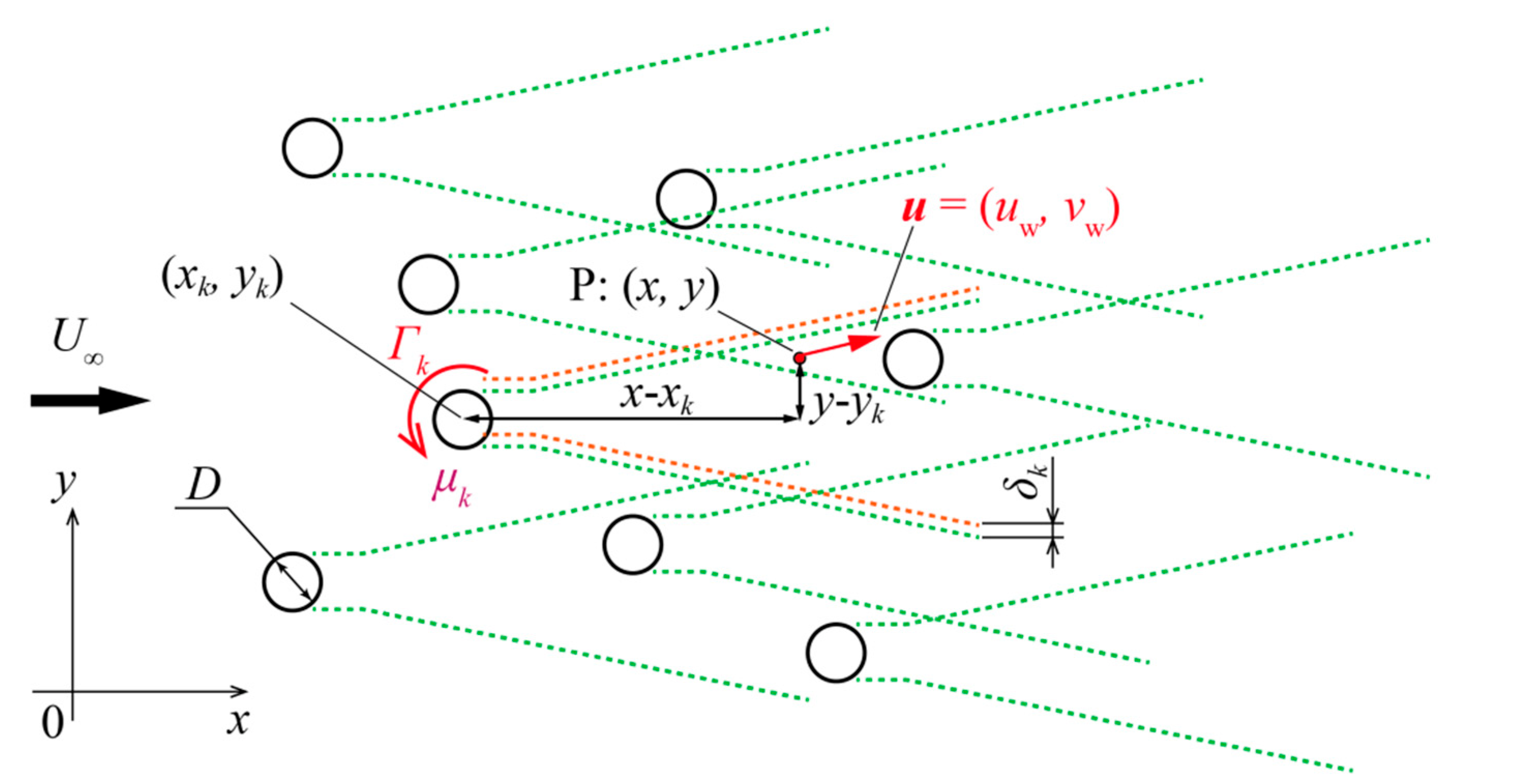
Figure 1 shows a schematic image of a VAWT wind farm, where a VAWT rotor is shown by a circle and our method does not need detailed information on the configuration of a turbine such as the number of blades and the cross-section. In our method, the VAWTs are dealt with as 2D rotors with each having a diameter, D. Let us assume the wind farm consists of N VAWTs. In Figure 1, the coordinate axis x is defined as parallel to the upstream wind speed U; the coordinate axis y is perpendicular to the dominant wind direction. The center position (rotational axis) of the k-th rotor is expressed as (xk, yk). Our method assumes that the circulation around an isolated single rotor (Γ) is given as a linear function of wind speed (U) in advance. Therefore, the blockage effect (dipole μ), thrust force (Th), and power output (P) are given as functions of the circulation, respectively, for each rotor.
If an arbitrary set of the conditions of circulation (Γk) and blockage effect (μk) is given for a wind farm, the complex velocity potential W(z), where z = x + iy is expressed by Equation (1) [23].
W z = U z + k = 1 N i Γ k 2 π ln z z k + μ k z z k 1
Using the above potential W(z), the potential flow (up, vp) at an arbitrary position P:(x, y) in the wind farm can be calculated as follows:
u p x , y = U k = 1 N Γ k 2 π y y k x x k 2 + y y k 2 + μ k x x k 2 y y k 2 x x k 2 + y y k 2 2
v p x , y = k = 1 N Γ k 2 π x x k x x k 2 + y y k 2 μ k 2 x x k y y k x x k 2 + y y k 2 2
However, the potential flow is an ideal flow and cannot express the actual velocity deficit or wake generated by each rotor. Therefore, as Whittlesey et al. introduced [23], the component in the x-direction of the potential flow is modified by a wake function duk showing the velocity deficit of each rotor; the resultant flow uw(x, y) is expressed by Equation (4). The subscript “w” means the flow field obtained by applying the wake function (or wake model) in this study.
u w x , y = u p x , y 1 k = 1 N d u k x , y
In our method, the wake function duk is given by Equation (5) including the ultra-super-Gaussian function fUSG_k defined in our previous study [37]. The function fUSG_k modifies the super-Gaussian function 𝑓SG_k proposed by Shapiro et al. [38] expressing the wake profile transformation from top-hat shape to Gaussian by adding the correction function 𝑓COR_k expressing the acceleration regions and the deflection δk of the wake. μref is a reference value of the blockage effect and CW_k is a fitting parameter to the prepared flow field of an isolated single rotor.
d u k x , y = C w _ k μ k μ ref f USG _ k = C w _ k μ k μ ref f SG _ k f COR _ k
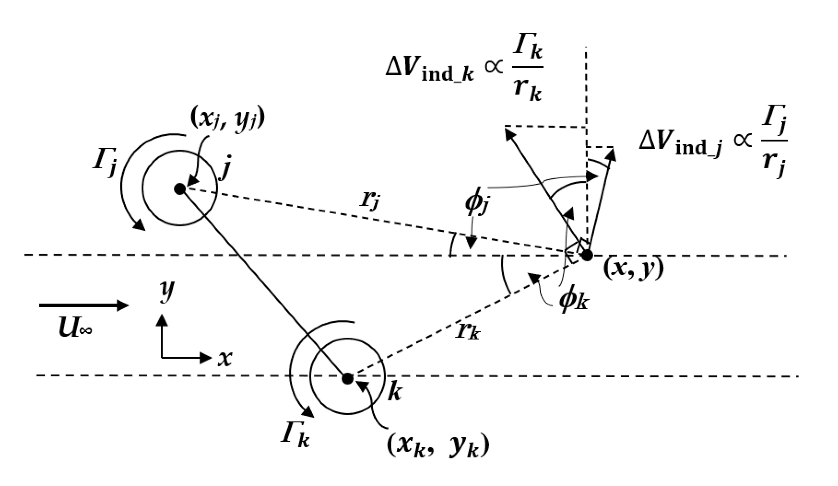
The present method modifies the wake deflection δk and the wake width dW, which are used in the ultra-super-Gaussian function 𝑓USG_k, by using the induced velocity given by the Biot–Savart law. The details are described in Appendix A.
The component in the y-direction of the potential flow is also modified by Equation (6) in our method [40].
v w x , y = v p x , y + U k = 1 N | Γ k | | Γ SI | d v k x , y
where dvk shows the difference in y-component velocity between the potential flow and the prepared flow (by CFD or experiments) around an isolated single rotor, the circulation of which is defined as ΓSI and depends on U (see Equation (A17) in Appendix B). The dvk is approximated using the sum of four Gaussian-type functions fG_i and four resonant-type functions fR_i as shown in Equation (7). The details of functions fG_i and functions fR_i are described in Appendix A.
d v k x , y = i = 1 4 f G _ i + i = 1 4 f R _ i
If an arbitrary set of circulations (Γk) of N rotors is given, a flow field and a set of rotor outputs are calculated by using Equations (2)–(7) and the prepared relation between the circulation and rotor power. However, the result is not always the actual correct condition. Therefore, we have to find out the set of circulations that give the condition satisfying the conservation of momentum expressed by Newton’s law of motion.
Figure 2 shows a schematic image of a control volume (CV) used for the calculation of the flow field around an isolated single rotor. The prepared data of an isolated single rotor, regardless of CFD data or experimental data, must satisfy Equation (8). The left-hand side of Equation (8) is the total force acting on the fluid in the x-direction (main flow direction) and the right-hand side shows the variation in the momentum in the x-direction per unit time. The variation in the momentum Δ m ˙ u x is calculated from the flow velocity at the boundaries of CV by Equation (9), in which the mass flow rate m ˙ x and m ˙ y are expressed by ρ u d y and ρ v d x , respectively. Here, ρ is the air density; dx and dy are small boundary elements. The total force F total _ x is given by Equation (10), in which the pressure forces Fpin and Fpout acting on the inlet and outlet boundaries are considered and are calculated by the integration along each boundary. The Fp in Equation (10) shows the total pressure force in the x-direction and means the pressure loss. The forces ( F _ τ _ top   ,   F _ τ _ bottom ) caused by shear stress on the top and bottom boundaries are neglected in this study. From Equations (8) and (10), the relation of Equation (11) is obtained for an isolated single rotor. In our method, the pressure loss Fp has to be prepared as a function of the upstream speed or the corresponding circulation of a single rotor for an applied CV. Note that the pressure loss Fp cannot be calculated from the model flow field obtained by using Equations (4) and (6).
F total _ x = Δ m ˙ u x
Δ m ˙ u x = m ˙ x u in + m ˙ x u out m ˙ y u bottom + m ˙ y u top
F total _ x = T h + p in d y p out d y = T h + F p in F p out = T h + F p
Δ m ˙ u x = T h + F p
To apply the momentum balance given by Equation (11) to a wind farm, an evaluation function Err is defined by Equation (12).
E r r = Δ m ˙ u x + k T h k k f p k F p k
where Thk and Fpk are the thrust force and pressure loss caused by the k-th rotor under the condition of an isolated single rotor, respectively. Thk and Fpk are calculated using the input value of circulation (Γk) based on the prepared information for an isolated single rotor. fpk is the correction function introduced to express the interaction between the k-th rotor and other rotors and is defined by Equation (13), in which I j is a function expressing the interaction effects from the j-th rotor to the k-th rotor.
f p k = 1 j k I j
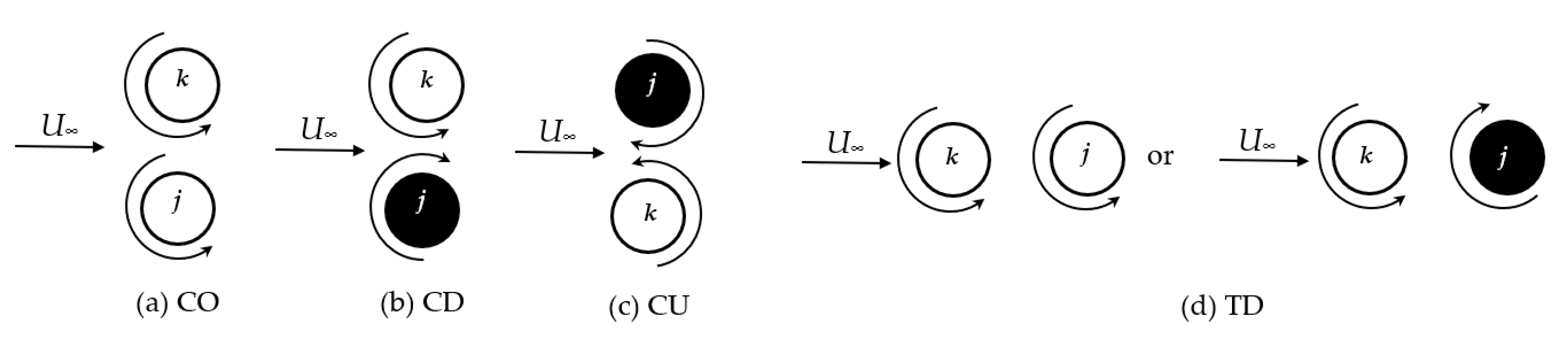
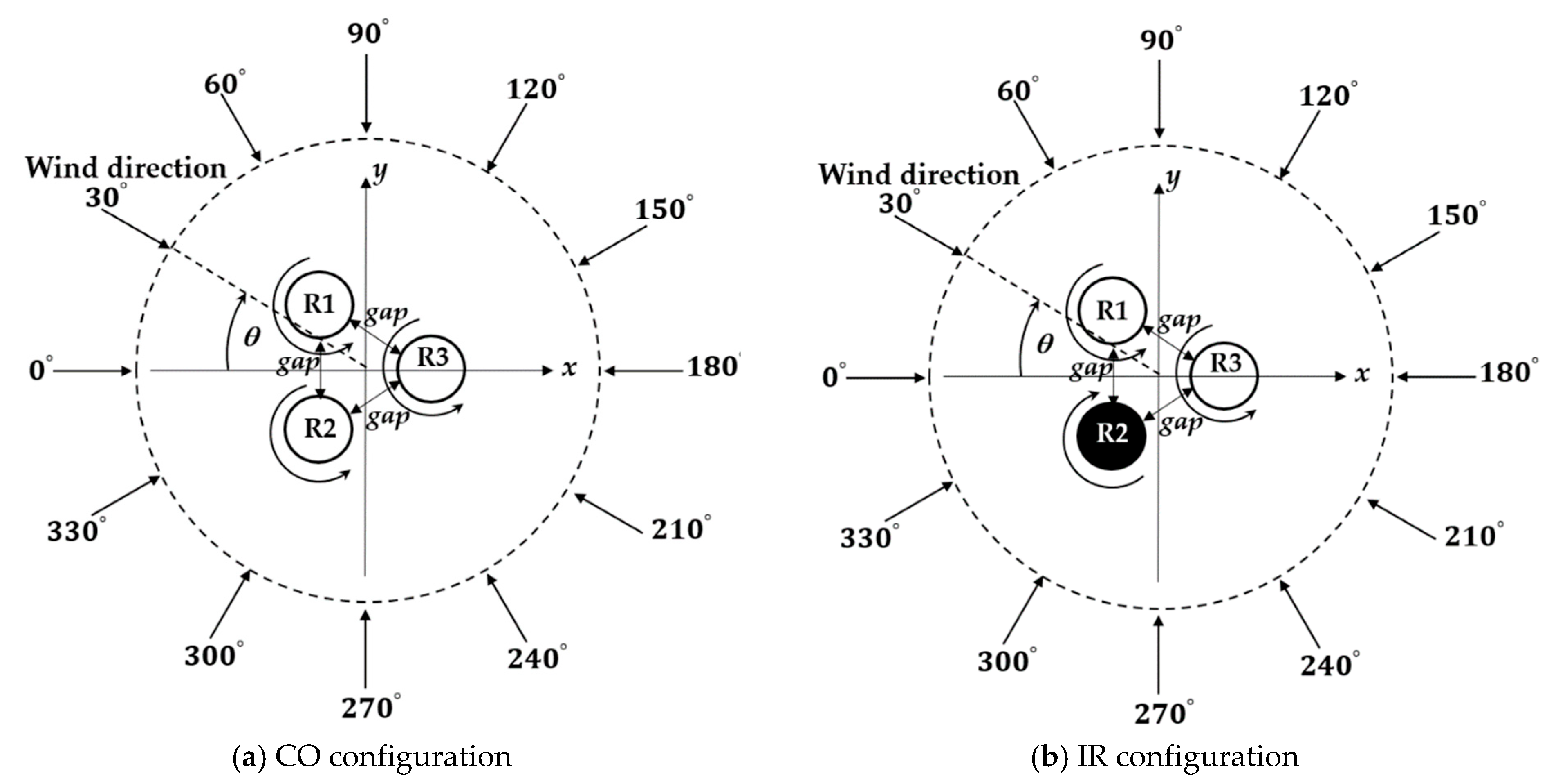
The layouts between selected two 2D-VAWT rotors can be roughly categorized into four kinds according to the relative rotation condition against the main flow U as shown in Figure 3; i.e., co-rotating (CO), counter-down (CD), counter-up (CU), and tandem (TD).
In our method, the interaction function I j 
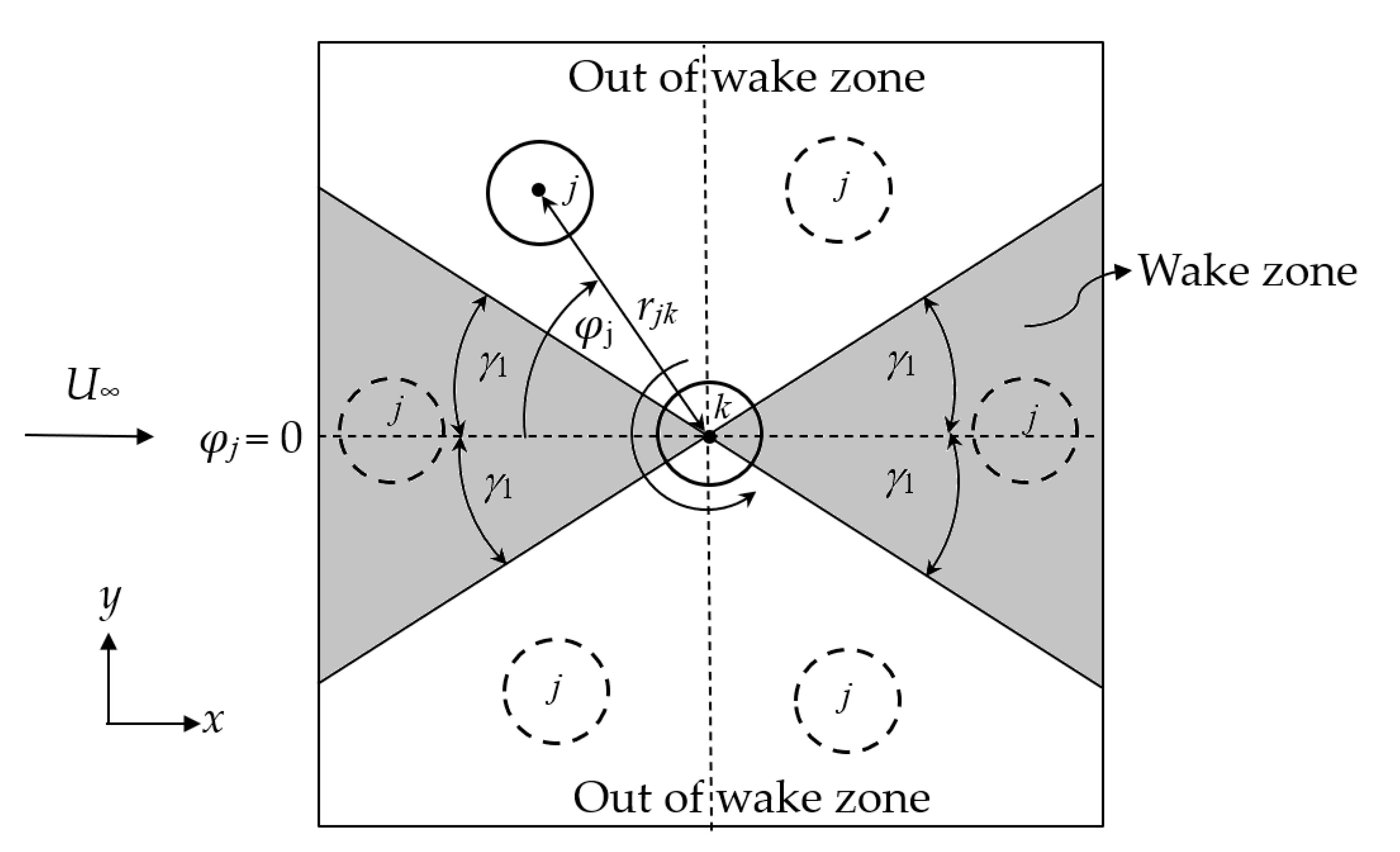
is defined separately for each category of the selected two-rotor layout as shown in Equations (14)–(17).
I j = α 1 Γ j Γ SI sin φ j D r j k 2         ; for   CO like
I j = α 2 Γ j Γ SI sin φ j D r j k 2         ; for   CD like
I j = α 3 Γ j Γ SI sin φ j D r j k 2         ; for   CU like
I j = α 4 Γ j Γ SI cos φ j D r j k 2         ; for   TD like
φ j is defined as the angle between the direction seen from the k-th rotor to the j-th rotor and the upwind direction as shown in Figure 4. r j k is the distance between the centers of the two rotors. A constant angle γ 1 divides the CV into two zones, i.e., the wake zone (in gray) and the out-of-wake zone (in white). If the j-th rotor (counterpart to the k-th rotor) exists in the wake zone, Equation (17) is used for the calculation of the interaction function I j as the TD-like layout. When the counterpart rotor exists in the out-of-wake zone, the equation used for the calculation of the interaction function I j 
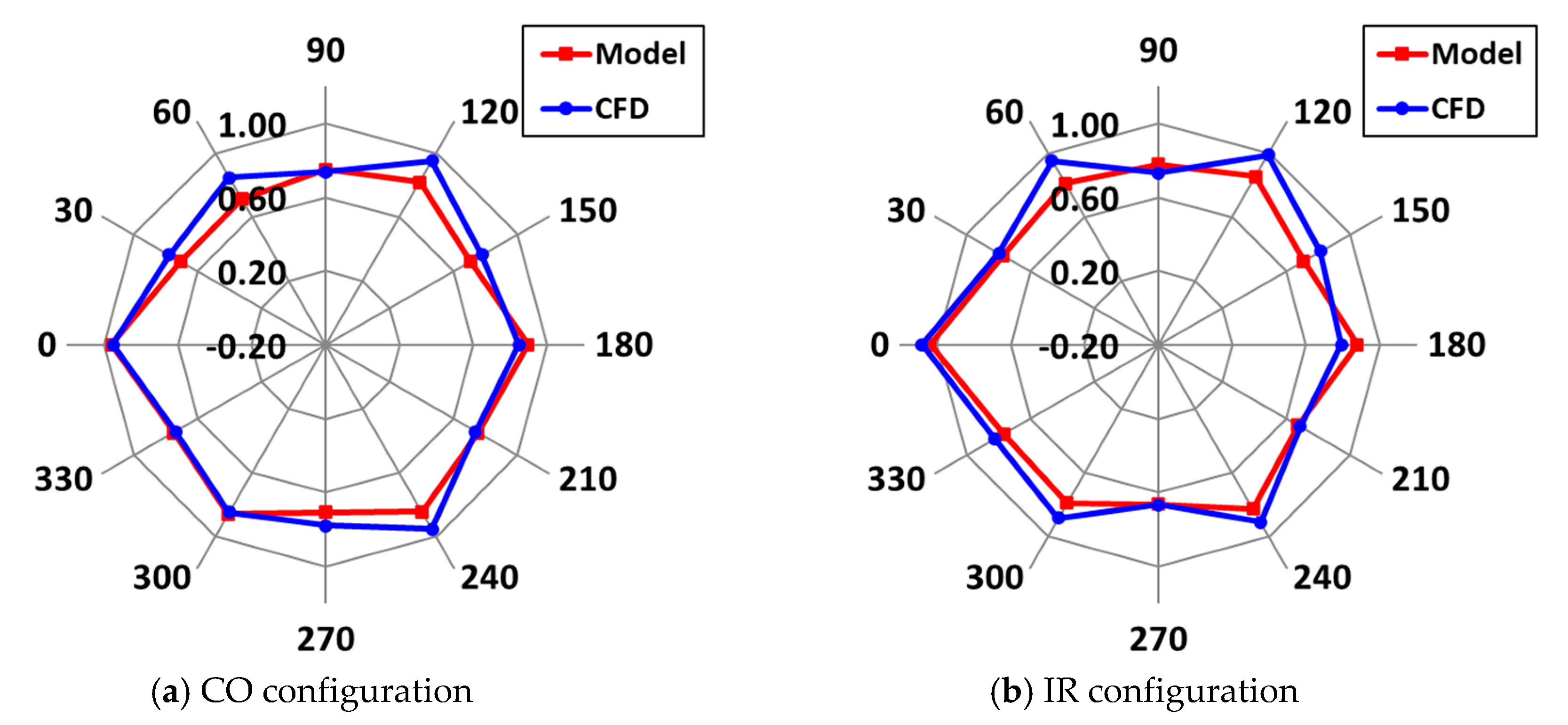
is determined as one of three equations (Equations (14)–(16)) according to the corresponding layout category of the two rotors. The fitting parameters of α 1 ,   α 2 ,   α 3 , and α 4 are introduced so as to obtain a sufficient correspondence between the results of rotor power prediction using the model and the CFD analysis, in the specific four conditions of paired rotors, i.e., CO, CD, CU, and TD layouts.
The flow chart of the method is shown in Figure 5. Before starting the calculation, the relations, such as between the circulation and rotor output, and the fitting parameters must be prepared from the information of an isolated single rotor and four specific conditions of two rotors. The first step of the actual model calculation is to decide the calculation conditions such as the upstream wind speed (U), the positions of the rotors, and the rotational directions. The input parameters are the fitting parameters obtained by comparison of the velocity distribution (x- and y-components) of the model with that of the CFD in the case of an isolated single rotor. For example, the fitting parameters include CN0, CN1, CN2, CN3, CP0, CP1, CP2, and 
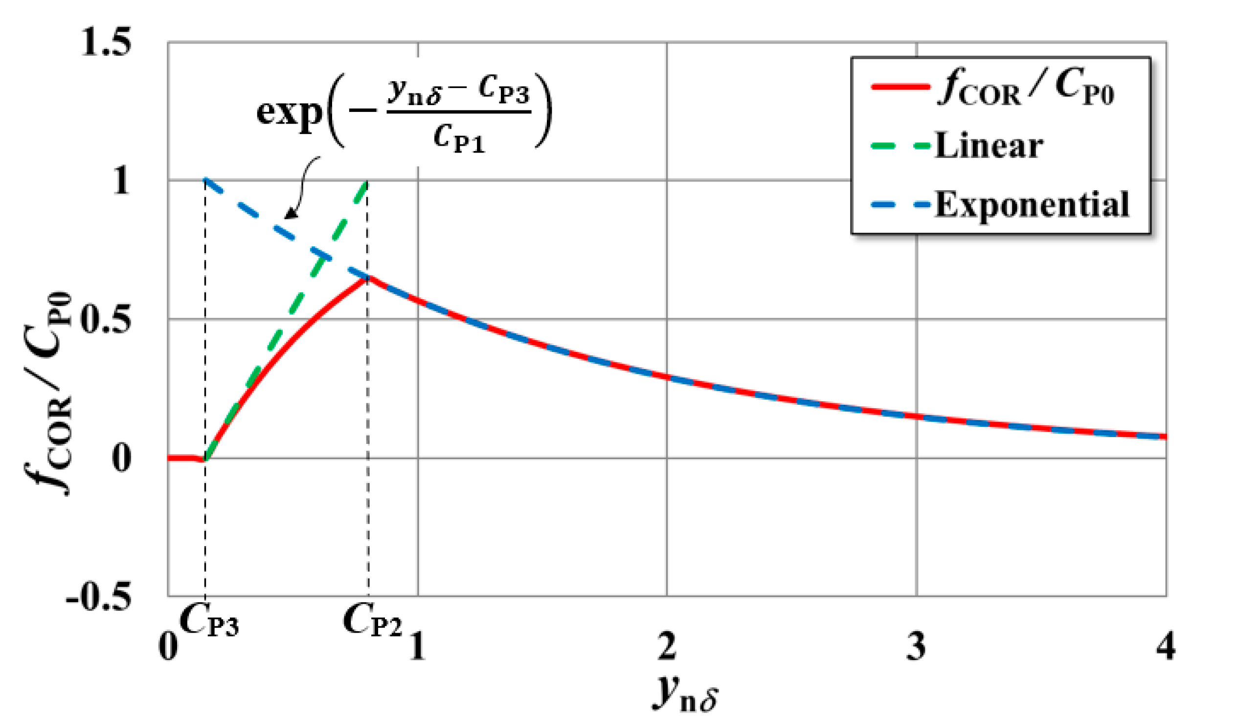
CP3, which are used to define the correction function fCOR of the ultra-super-Gaussian function and are defined in Equations (A4)–(A9) in Appendix A. The fitting parameters must be determined at several positions in the flow field according to the complexity of the local velocity profiles. The present study uses 35 parameters. All the fitting parameters are shown in Table A1, Table A2, Table A3, Table A4, Table A5 and Table A6 of Appendix A. After the initial condition of the rotors and a set of parameters are input, the process of searching for a reasonable combination of circulations is initiated starting from the lowest value of the circulation in a given searching range for each rotor (determining the searching ranges will be described in Section 2.2). For a given combination of circulations, the potential flow is calculated first and it is modified by our wake model to include the effects of the velocity deficits. With the flow field (uw, vw) obtained, the momentum changes in the x-direction per unit of time Δ m ˙ u x is calculated from the four boundary conditions. The thrust force Thk and the (isolated single rotor) pressure loss Fpk are calculated by Equations (A19) and (A20) in Appendix B by using the given circulation value for each rotor. Using the interaction function I j , the correction function fpk which expresses the effects of the inter-rotor interaction is obtained for each rotor by Equation (13). Then, the momentum balance Err is evaluated by Equation (12). The “error” of momentum balance is defined in Equation (18) in the present study. The denominator in Equation (18) is the momentum per unit time entering into the CV from the inlet boundary.
e r r o r = E r r 2 m ˙ x u in
The above calculation is repeated by changing the combination of circulations with the interval of ΔΓ throughout all the searching ranges. After the round robin, a combination of circulation Γk which gives the smallest “error” is obtained. In the present study, the similar searching process (sub-searching) is repeated twice by narrowing the searching ranges as (Γk − ΔΓ) Γk_i  (Γk + ΔΓ). Finally, for the smallest “error” condition, the power output of each rotor can be obtained by using Equation (A21) in Appendix B.

2.2. Specific Calculation and Searching Range of Circulation

In this section, we consider a specific case assuming small rotors in order to explain the selection of searching range to obtain adequate circulation. The target rotors are the same as those investigated in the previous study [35] and the rotor configuration is depicted in Figure A4 in Appendix B. The necessary relations on the performance of the single rotor are given in Equation (A17)–(A20). The values of α 1 ,   α 2 ,   α 3 , and α 4 were determined as 0.2304, 0.19, −0.2853, and 1.07, respectively, from the preliminary calculations of the specific four layouts of paired rotors. The CV was defined as 20D × 20D × 0.868D. The thickness of the CV given by 0.868D corresponds to the rotor height of the target rotor; by considering the rotor height, our 2D method can be applied to the prediction of the power output of an actual 3D-VAWT rotor.
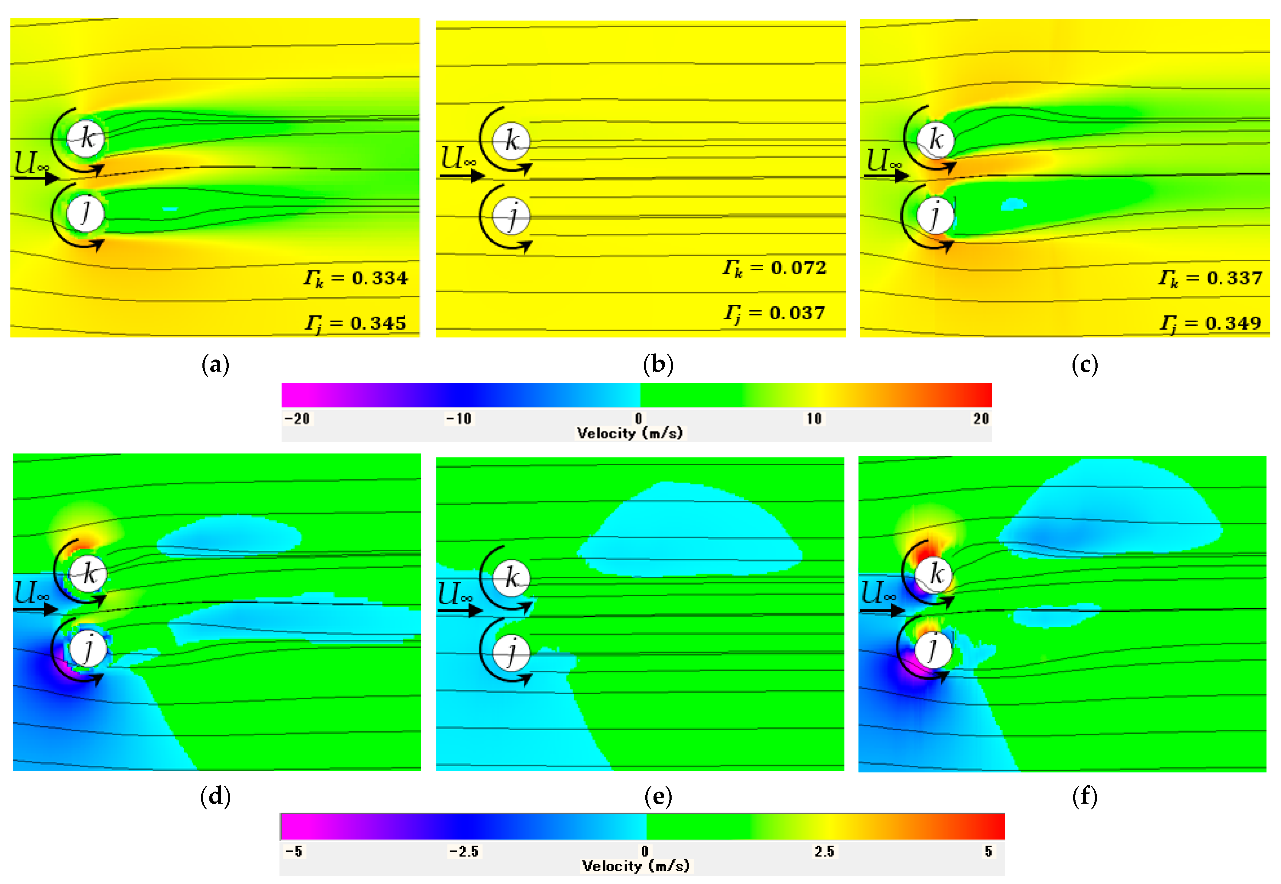
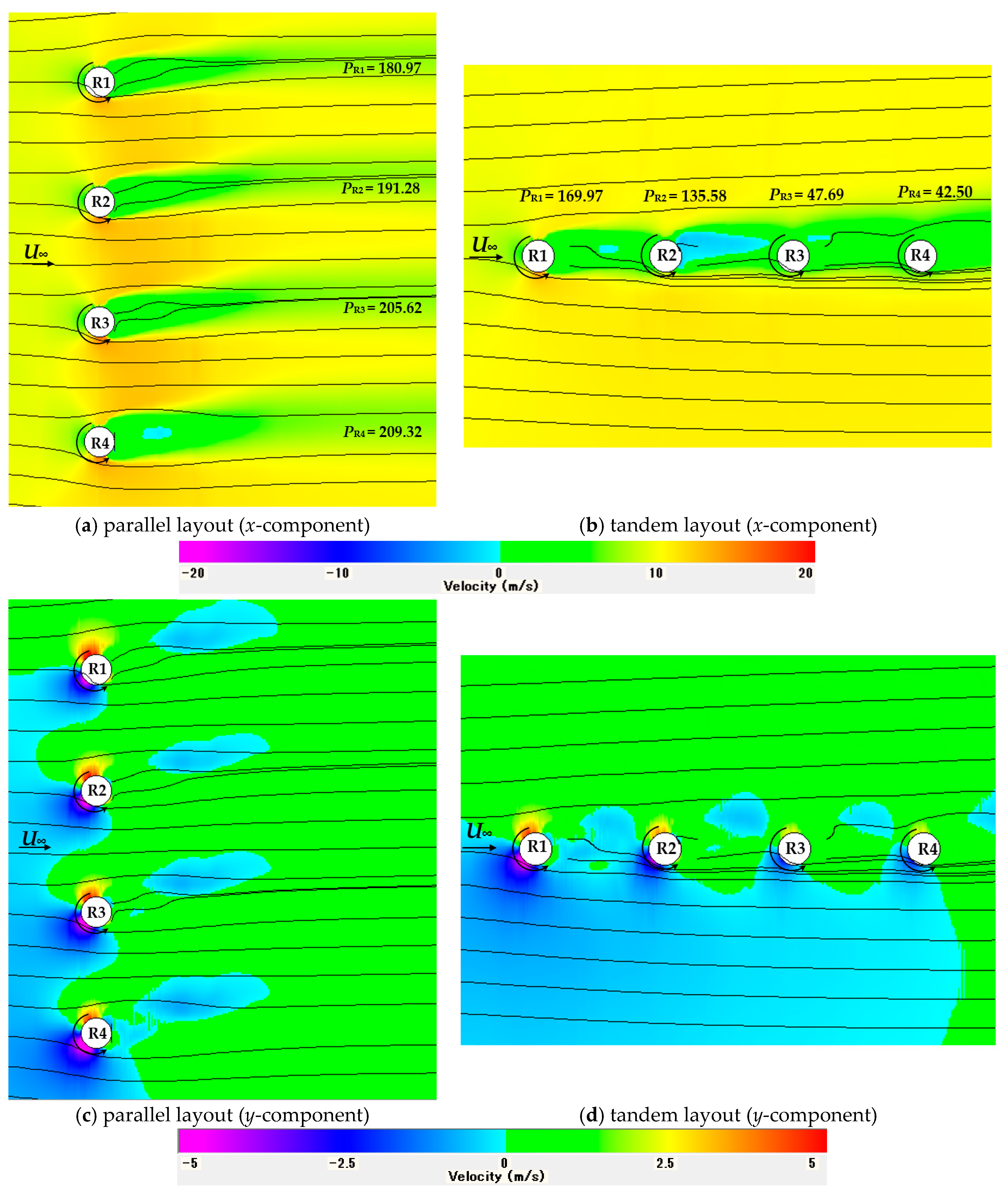
Figure 6a,d show the averaged distributions of the x- and y-component velocities calculated by the CFD analysis around two VAWT rotors rotating CCW direction in the CO-like layout. The commercial code STAR-CCM+ was utilized for the CFD simulation. The circulation of the upper rotor (rotor-k) is 0.334 m2/s, which was obtained by the integration of the flow field along a circular path at r/D = 0.75. The circulation of the lower rotor (rotor-j) is 0.345 m2/s. The details of the rotor shape are not shown but are replaced by circles in white in Figure 6a. The black solid lines around the rotors are path lines.
Figure 6b,e show the resultant flow field obtained by the proposed method using an in-house code, in which the circulation of each rotor was changed step by step in a round robin over a wide searching range from 0.1 Γ SI to 1.1 Γ SI . Here, Γ SI is the circulation of an isolated single rotor obtained from the CFD analysis and the value is 0.326 m2/s in the case of U = 10 m/s. The obtained circulations of two rotors in Figure 6b are Γk = 0.072 m2/s and Γj = 0.037 m2/s, respectively, and they are different from the CFD results in Figure 6a. To demonstrate the variation in the error of momentum balance graphically, we define a new indicator (1 − error) that approaches 1 when the error becomes small. The distribution of the values of (1 − error) obtained in the searching process of the smallest error in the case of Figure 6b is shown in Figure 7, which includes 625 results corresponding to the combinations of circulation values (Γj, Γk) with the interval of (1.1 − 0.1) Γ SI /25. Figure 7 shows that there are a lot of combinations of circulation which might give a small error.
In the parallel layouts, it is expected that two rotors have large circulations close to the value of Γ SI . Therefore, the search range can be narrowed. Figure 6c,f are is the flow field obtained using a searching range limited from 0.95 Γ SI to 1.1 Γ SI for each rotor in the CO layout. The circulation combination giving the smallest error, shown in Figure 6c, is Γk = 0.337 m2/s and Γj = 0.349 m2/s, respectively. 
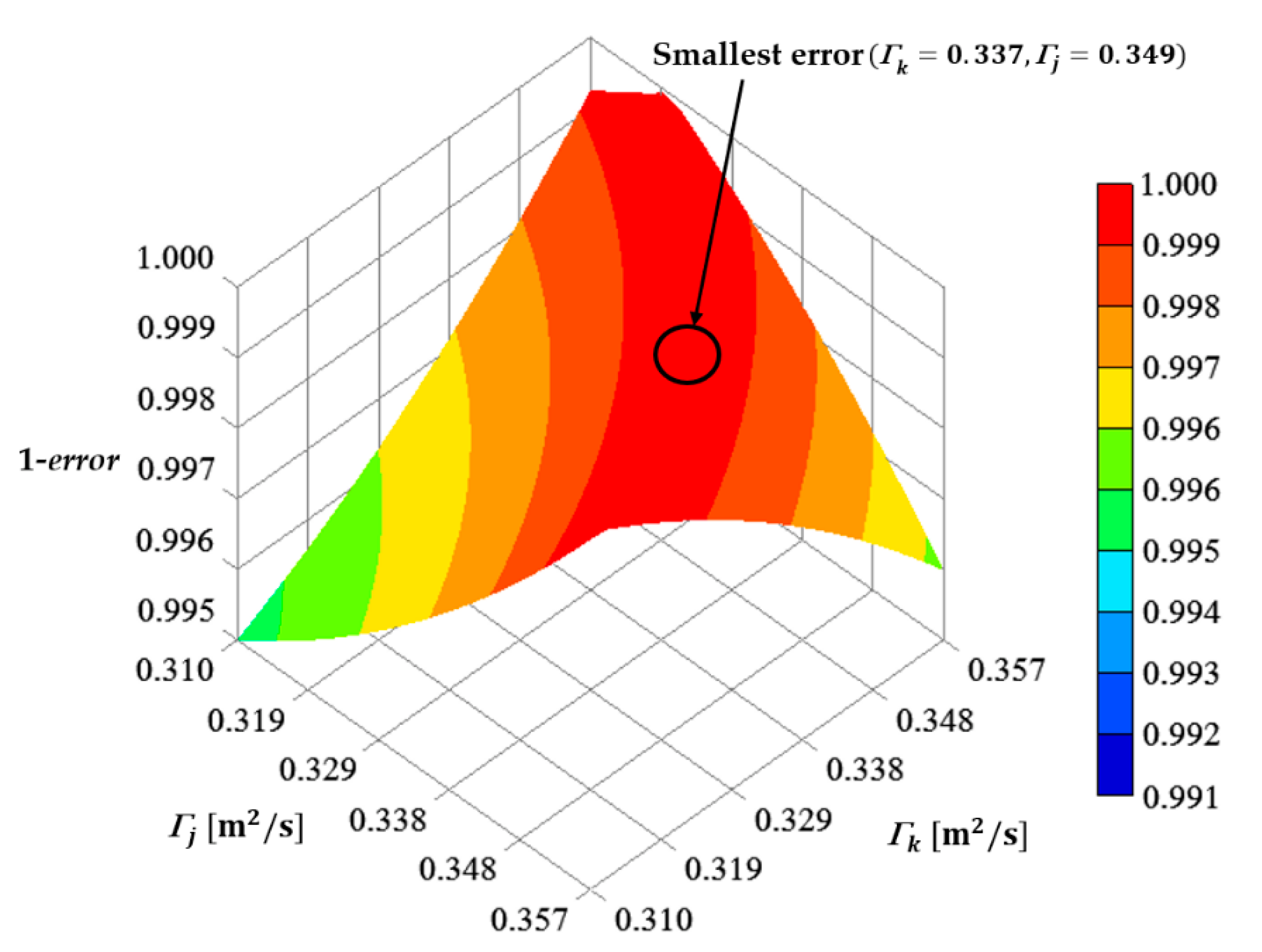
Figure 8 is the distribution of the 625 values of (1 − error) obtained in the searching process with a limited range from 0.95 Γ SI to 1.1 Γ SI for each rotor. The results of our method with appropriately limited searching ranges can approach the CFD results.
Incorrect results are also obtained when the rotor at issue exists in the wake of other rotors if the wide searching range of circulation is applied. In our method, we propose a procedure to search for the appropriate result close to the CFD result, in which the searching range of circulation of each rotor in a VAWT wind farm is limited in the manner described below.
Let us define a circular region of the radius Rint around a rotor (k) at issue, and assume there are Nint rotors in the region. We consider that only the rotors (j) included in the interaction region defined by Rint are used to decide the searching range of circulation of the rotor (k).
First of all, the angle φ j defined in Figure 4 is checked for all rotors in the interaction region. If the absolute value of one of the angles is less than a constant angle γ 2 , the searching range expressed by Equation (19) is applied. Note that the angle γ 2 is different from the angle γ 1 , and γ 2 is less than γ 1 . The interaction region is determined to be a circle of Rint = 10D in this specific calculation; therefore, the maximum of the inter-rotor distance (between rotor centers) rjk is 10D in Equation (19) in this study.
0.3 Γ SI Γ k < 0.075 r j k D + 0.35 Γ SI           ;         for         φ j < γ 2
In the second step of the procedure, the average of the distance dj between the center of the j-th rotor and the stream-wise center line through the k-th rotor at issue is calculated with all the counterpart rotors of the k-th rotor in the interaction region using Equation (20).
d j ¯ = j k d j N int 1
In the third step of the procedure, the searching range of the circulation Γk of the k-th rotor is determined as one of Equations (21)–(23) according to the averaged lateral distance d j ¯ . Figure 9 schematically shows the definition of the angle γ 2 and three zones determining the searching range of circulation of the k-th rotor. The delimiting lateral distances are determined as d1 = 0.9D and d2 = 1.5D in this study.
0.85 Γ SI Γ k < 1.0 Γ SI           ;             for         0   d j ¯ < d 1
0.9 Γ SI Γ k < 1.0 Γ SI           ;             for   d 1 d j ¯ < d 2
0.95 Γ SI Γ k < 1.1 Γ SI           ;             for   d j ¯   d 2

3. Results and Discussion

The method described in Section 2 is validated in this section by applying it to several layouts consisting of the same small 2D rotors as used in the previous section (Section 2.2). Firstly, in Section 3.1, the power dependency of the isolated single rotor on the wind speed is confirmed. Then, in Section 3.2, the power dependency of the paired rotors on the 16 wind directions is compared between the present method and the CFD analysis obtained in the previous study. As for the more complicated layouts, the power dependency of the three-rotor cluster on the 12 wind directions is investigated in Section 3.3. Finally, to show the applicability of the proposed method to VAWT wind farms, the power prediction in the four-rotor layouts arranged in a line is tried in Section 3.4.

3.1. An Isolated Single Rotor

Table 1 shows the comparison between the CFD analysis [35] and the model simulation using the present method based on the momentum balance in the cases of an isolated single rotor in the five different upstream wind speeds (U). Although the original CFD analysis was conducted using a wide calculation domain of 40 D × 50 D, the square region of 20 D × 20 D enclosing the single rotor is extracted as the CV, which is the same size as that of the model simulation, in order to acquire the dependence of the pressure loss Fp on the circulation of the isolated single rotor. The output power shown in the unit of “mW” is equivalent to that of the small rotor, the size of which is 50 mm in diameter × 43.4 mm in height. The parameters necessary to rebuild the flow field calculated by the CFD were obtained at the reference wind speed of U = 10 m/s. Therefore, the smallest percentage difference (% Error) between the model and CFD results is obtained in the case of U = 10 m/s. The output power predicted for a single rotor in other wind speeds agrees well with the CFD result; this means the method using momentum conservation works well.

3.2. Paired Rotors

In this section, the prediction of the powers of paired rotors is investigated. Figure 10 shows the definition of relative wind direction ( θ ) to the rotor pair which is categorized into two configurations in terms of the relative rotational direction of two rotors. The configuration in Figure 10a is defined as the co-rotation (CO), which includes the CO and TD layouts where two rotors rotate in the same direction (see Figure 3). On the other hand, the configuration in Figure 10b is defined as the inverse rotation (IR), which includes the CD, CU, and TD layouts where two rotors rotate mutually in opposite directions. The dotted lines in red in Figure 10 correspond to the boundaries of the wake zone defined by the angle γ 1 in Figure 4. The angle γ 1 is set at 30° in this study.
The power outputs of the upper (Rotor 1: R1) and lower (Rotor 2: R2) rotors and the averaged power of both rotors were predicted in each of the 16 wind directions by the present method under the condition of the upstream wind speed U of 10 m/s. The results in the case the inter-rotor space (gap) is equal to the rotor diameter are shown in Figure 11a–c for CO and Figure 12a–c for the IR configurations. Each of the predicted rotor power is normalized by the power of the isolated single rotor (SI) and compared with the normalized CFD results in Figure 11 and Figure 12. The conditions of θ = 0° and 180° in Figure 11c are the same CO layout and their output powers were adjusted to agree with the CFD results to get the adequate value of the parameter α 1 . The conditions of θ = 0° and 180° in Figure 12c correspond to the CD and CU layouts, respectively, and the values of the parameters α 2 and α 3 were adjusted so as to agree with the CFD results. Similarly, the conditions of θ = 90° and 270° in Figure 11c and Figure 12c correspond to either of the two TD layouts shown in Figure 3d, and the parameter α 4 can be determined by fitting the resultant circulations obtained by the model simulation to those of the CFD analysis in one of the four TD conditions. The actual values of α 1 ,   α 2 ,   α 3 , and α 4 were already shown in Section 2.2. Although the difference between the model simulation and the CFD analysis is somewhat large in a few wind directions as shown in Figure 11 and Figure 12, the method can predict the power of a rotor pair with the gap = 1.0D very well.
Figure 13 and Figure 14 are the results of the rotor power distribution of the paired rotors with the gap = 0.5D. The model simulation seems to underestimate the rotor powers compared with the CFD analysis in many wind directions.
Figure 15 and Figure 16 show the results in the case of gap = 2.0D. Except for a few directions, the model and CFD predictions agree well in the long inter-rotor distance case. This fact may suggest the necessity to modify the interaction function I j defined in Equations (14)–(17) in the case of short inter-rotor distance.
Although further improvements may be needed in the present method, it is worth noting that the prediction of the power of paired rotors in a specific wind direction can be performed by the method in about 40 min, which is 500 times shorter than the calculation time with the CFD analysis using the DFBI model (about 2 weeks).

3.3. Three-Rotor Cluster

The three-rotor cluster is also categorized into the CO and IR configurations. Figure 17 shows the definition of the 12 wind directions for the two configurations in the cases of three-rotor clusters which are arranged like a triangular shape with an inter-rotor space of gap = 1.0D. Under the condition of the upstream wind speed U of 10 m/s, the prediction of the averaged output power of the rotor clusters was carried out. All the parameters and necessary relations such as the pressure loss function are the same as those used in the case of paired rotors except for the division of the searching range of circulation. The number of divisions of the searching range was set as 10 in the three-rotor case instead of the 25 used in paired rotors case to save the calculation time. Therefore, the error in the prediction is anticipated to be a little worse.
Figure 18 is the prediction results of the averaged power of the three rotors. The model calculation underestimates the averaged power of the rotor clusters. However, the dependence on the wind direction is well simulated and the model simulation gives the same trend as the CFD analysis [41].

3.4. Four-Rotor Layout

Finally, to show the applicability of the proposed method to VAWT wind farms, four-rotor layouts arranged in line with an inter-rotor space of 3.0D were selected as the targets of the output power prediction. To cover a large number of rotors, the CV was set to be a large size of 40D × 40D × 0.868D. As the size of the CV was changed, the function expressing the pressure loss Fp of the CV was newly prepared from the CFD flow field of the isolated single rotor; i.e., the reference value Fpref in Equation (A20) in Appendix B was changed from 229.61 to 347.95 mN. The upstream wind speed was assumed to be 10 m/s. The number of divisions of the searching range of the circulation of each rotor was set as 8. In this case, the calculation time is about 50 times as long as the calculation time in a two-rotor case with the 25 division because the subdivision process is executed twice in the actual calculation using the in-house code.
Figure 19a–d show the results of the power prediction and the distributions of x- and y-direction velocity components in two kinds of four-rotor layouts, i.e., parallel and tandem, respectively. The fitting parameters α 1 ,   α 2 ,   α 3 , and α 4 are set to be the same values as those used in the paired rotors (see Section 2.2). The model predicts the decrease in the rotor power in the order of R1, R2, R3, and R4 in the parallel array of four rotors. Similarly, in the tandem array of four rotors, the output power decreases in the same order.
In this study, the CFD analysis of the two kinds of four-rotor layouts was carried out by using the DFBI model. The mesh size and whole domain size of each simulation of the four-rotor layouts are the same as those used in the previous CFD analysis of one-, two-, and three-rotor arrangements. The details of the meshes created for the four-rotor layouts in the present study are shown in Appendix C. The upstream wind speed U is set at 10 m/s in the CFD analysis of four-rotor layouts.
Figure 20a,b show the distributions of x-component of unsteady velocity obtained by the CFD for the parallel and tandem layouts, respectively. Figure 20c,d illustrate the unsteady flow field shown by the y-component velocity for the two layouts of four rotors. The condition shown in Figure 20 corresponds to the state at 4 s from the beginning of the simulation. The time history of the angular velocity of each rotor is shown in Appendix C. The CFD analysis was conducted by a high-performance PC with 28 cores; it took about 1 week for each calculation of two layouts.
Table 2 shows the comparison of each rotor power in the parallel and tandem layouts between the present model and CFD analysis. The percentage error of the rotor power (Err.P) is defined by Equation (24) in this study. PModel is the rotor power predicted by our model using Equation (A21) and the PCFD is the CFD result of the rotor power which is obtained by multiplying the averaged angular velocity and the averaged rotor torque during the last 0.5 s. The Pref is the output power of an isolated single rotor.
E r r . P = P Model P CFD P ref × 100
The comparison shown in Table 2 does not give satisfactory results. In particular, the difference between the model and CFD is large in the tandem layout of four rotors. One of the reasons for the disagreement is the small number of initial divisions of the searching range used for the model prediction. An advanced method like the genetic algorithm (GA) should be used to give the possible combinations of circulations at random. Further improvement in the model of the interaction among rotors also is necessary. Nevertheless, the present model can predict the same trend in the rotor power in the parallel and tandem layouts of four rotors as that of the CFD analysis.

4. Conclusions

We developed a method to predict the output powers of the vertical-axis wind turbine (VAWT) rotors of an arbitrary layout; the calculation time can be incomparably shorter than computational fluid dynamics (CFD) using the dynamic fluid/body dynamics (DFBI) model, which enables the time variation in rotor speed. However, our method needs to know information, such as the flow velocity distributions and pressure loss and circulation, and so on, around an isolated single rotor in several wind speed conditions. In addition, four fitting parameters must be determined in advance to express the interaction effects between two rotors in the CO, CD, CU, and TD layouts having a specific inter-rotor space (gap). By applying the law of the momentum conservation with including the interaction effects through the modification of the pressure loss of the control volume (CV), the method could predict the power dependence of the paired rotor with the rotor gap of 1.0D on the 16 wind directions, which agreed with the CFD analysis well. However, the dependence on the inter-rotor distance (between rotor centers) should be improved. The application of the method to the three-rotor cluster showed almost the same trend as the CFD in the averaged power distribution over 12 wind directions. The method was applied to the four-rotor layouts arranged in line of parallel or tandem to the main flow to show the applicability to VAWT wind farms. The important advantages of our method include the very small number of the calculation grid (actually 400 × 400 used) and the random positioning of rotors as well as the significantly short calculation time compared with the CFD using the DFBI model. Unlike the conventional wake models, our wake model can express the acceleration regions existing on both sides of the velocity deficit. Once the necessary parameters are prepared, the averaged flow field around an arbitrary rotor layout of the VAWT cluster can be reproduced with fidelity as high as the CFD analysis. To apply our method to the problem of finding the optimal layout of rotors in a VAWT wind farm, it is necessary to increase the accuracy of the prediction and to introduce other optimization methods such as the genetic algorithm (GA) instead of the round robin.

Author Contributions

Conceptualization, Y.H.; methodology, J.B. and Y.H.; software, J.B. and Y.H.; validation, Y.H.; formal analysis, J.B. and Y.H.; investigation, J.B.; resources, J.B. and Y.H.; data curation, J.B.; writing—original draft preparation, J.B.; writing—review and editing, Y.H., M.F. and Y.J.; visualization, J.B.; supervision, Y.H.; project administration, Y.H.; funding acquisition, Y.H., M.F. and Y.J. All authors have read and agreed to the published version of the manuscript.

Funding

This research was supported by JSPS KAKENHI Grant Number JP 18K05013, the International Platform for Dryland Research and Education (IPDRE), Tottori University, and the 2021 Special Joint Project of the Faculty of Engineering, Tottori University.

Data Availability Statement

The data that support the findings of this study are available from the corresponding author, J.B., upon reasonable request.

Acknowledgments

The first author thanks Tomoyuki Okinaga at Tottori University for helping with the CFD simulation. The authors thank the Advanced Mechanical and Electronic System Research Center (AMES) for supporting the article processing charge.

Conflicts of Interest

The authors declare no conflict of interest.

Appendix A

Shapiro et al. [38] proposed the super-Gaussian function fSG which simulates the transformation of the wake profile (x-component of velocity deficit) of a horizontal-axis wind turbine (HAWT) from a top-hat shape to a Gaussian shape. We utilize the super-Gaussian function to simulate the wake profile of VAWT. However, the function cannot express the acceleration regions existing on both sides of the velocity deficit. Therefore, in our model, the correction function fCOR is introduced to express the acceleration regions [37,40]. In addition, the deflection of the wake of VAWT is considered.
Figure A1 compares the four profiles of the x-component velocity in the wake of an isolated rotor at xn = 2.0 [37]. As shown in Figure A1, the ultra-super-Gaussian function fUSG which subtracts the correction function (see Figure A2) from the super-Gaussian function fSG can reproduce the profile obtained by the CFD. Note that the super-Gaussian function fSG and the ultra-super-Gaussian function fUSG are defined as the profile of the velocity deficit.
Figure A1. Comparison of the profiles of the x-component velocity of the wake of an isolated rotor at xn = 2.0 (reproduced with permission from Buranarote et al. [37]).
Energies 15 05200 g0a1
Figure A2. Correction function for positive range in ynδ. (reproduced with permission from Buranarote et al. [37]).
Energies 15 05200 g0a2
The super-Gaussian function is expressed by the following Equation (A1):
f SG = exp D 2 8 σ 0 2 2 y n δ D d w x n p x n
where σ0 = D/4. In our model [37], the function p(xn) is defined as the following Equation (A2):
p x n = 2 1 + f p / x n
Here, xn is the non-dimensional coordinate defined by xn = (xxk)/D. fp is one of the fitting parameters, which is not included in the original super-Gaussian function. The normalized coordinate ynδ, which includes the wake shift δ, in Equation (A1) is defined as Equation (A3)
y n δ = y y k δ k D
The correction function f COR for y n δ   0 is defined as follows:
f COR = 0                       for   0 y n δ < C P 3
f COR = C P 0   exp y n δ C P 3   C P 1 1   C P 2 C P 3 y n δ C P 3        for   C P 3 y n δ C P 2
f COR = C P 0   exp y n δ C P 3   C P 1           for   y n δ > C P 2
In the region y n δ < 0 , the correction function f COR is given by Equations (A7)–(A9):
f COR = 0            for   C N 3 < y n δ < 0
f COR = C N 0   exp y n δ + C N 3   C N 1 1   C N 2 C N 3 y n δ + C N 3      for   C N 2 y n δ C N 3
f COR = C N 0   exp y n δ + C N 3   C N 1            for   y n δ < C N 2
In the present method, the wake deflection δk in Equation (A3) is modified by Equation (A10) to consider the interaction between rotors with the induced velocities uind (Equation (A11)) and vind (Equation (A12)) given by the Biot–Savart law. The distance rj and angle ϕ j are defined in Figure A3. Factors β 1 and β 2 are the correction constants. The sign of the second term in parentheses in Equation (A10) depends on the rotational direction of the selected two rotors and is positive when the rotors rotate in the same direction. The sign in front of the induced velocity vind in the index of the exponential function in Equation (A10) is positive when the k-th rotor rotates counterclockwise.
The wake width dW, which is used in the super-Gaussian function 𝑓SG_k [38], is defined by Equation (A13) in our method. kW is one of the fitting parameters in our method. The function α including a correction constant β 3 is defined by Equation (A14), in which the summation of the induced velocity does not include the effect from the k-th rotor.
δ k = Γ k Γ SI δ SI 1 ± 1 β 1 u ind v ind 1 e x x k / β 2 D 1 ± v ind
u ind = j Γ j r j sin ϕ j
v ind = j Γ j r j cos ϕ j
d w x n = 1 + k w ln 1 + e 2 1 + α x n
α = β 3 j k Γ j r j sin ϕ j
Figure A3. Schematic image of a pair of rotors and the induced velocity. Angle ϕ j is defined at an arbitrary point P:(x, y) when seeing the direction of the center position of a rotor on the basis of the upstream direction.
Energies 15 05200 g0a3
The non-dimensional function dvk for the y-component velocity correction is expressed by the superposition of four Gaussian-type functions fG_i and four resonance-type functions fR_i as shown in Equation (7). The Gaussian-type function and resonance-type function are defined by Equations (A15) and (A16), respectively.
f G _ i = C 1 fg _ i   exp y n δ C 3 fg _ i 2 C 2 fg _ i         ;   i = 1   to   4
f R _ i = C 1 fr _ i 1 + C 2 fr _ i y n δ C 3 fr _ i 2                 ;   i = 1   to   4  
There are 11 fitting parameters (Cw, kw, fp, CN0, CN1, CN2, CN3, CP0, CP1, CP2, and CP3) in fUSG, the values are shown in Table A1 and Table A2. There are 24 fitting parameters (C1fg_i, C2fg_i, C3fg_i, C1fr_i, C2fr_i, and C3fr_i; [i = 1 to 4]) in function dvk, the values are shown in Table A3 and Table A4 for the functions fG_i and Table A5 and Table A6 for the functions fR_i. The fitting parameters are determined at 46 positions between xn = −10 and xn = 10 in the x-direction by comparison between the velocity profiles of the model and the CFD result. At an arbitrary x-position in the flow field, the parameters are used for interpolation.
Table A1. The fitting parameters in the ultra-super-Gaussian function, fUSG, (xn < 0).
xnCwkwfpCN0CN1CN2CN3CP0CP1CP2CP3
−100.00910.65820.70100.25420.90570.20540.18450.43612.10680.21560.1880
−80.01140.69050.0993−0.47454.74722.67591.12210.23260.78570.46520.1646
−60.01680.79321.3848−0.55365.53773.12151.30900.14820.90120.58730.0326
−40.02740.90920.8591−0.39567.75061.40800.5688−0.06441.66393.38200.4386
−20.07680.74490.3266−0.63071.89312.01420.79560.158215.55375.71602.4223
−10.18260.78980.0532−0.29611.07241.45560.88660.107013.84693.34431.4025
−0.750.27720.59710.0423−0.34720.72441.41330.73440.08789.82892.89711.5263
−0.70.30000.60010.0161−0.43800.57241.66830.76540.084912.33163.05270.4652
−0.60.28820.63300.0552−0.28690.62561.35190.77410.10089.78762.67590.5537
−0.50.32820.55570.0002−0.30870.57151.29860.60400.10427.46382.54090.7335
−0.40.28870.50190.0501−0.30790.44661.14600.65430.13256.58291.94130.8771
−0.30.42350.23100.0501−0.27390.37180.99420.51100.10355.98611.63610.7088
−0.20.67540.20620.4530−0.26980.34800.17110.17110.07975.27131.29410.3692
−0.10.62320.03340.1954−0.09350.20870.51960.51960.10744.50320.24340.2433
Table A2. The fitting parameters in the ultra-super-Gaussian function, fUSG, (xn  0).
xnCwkwfpCN0CN1CN2CN3CP0CP1CP2CP3
00.54280.00020.05030.03763.29771.85890.41960.15753.62270.25870.2586
0.10.65770.00020.39360.06362.39791.70940.00050.17133.04110.21620.2161
0.20.70260.00020.81190.05692.78570.96080.08700.18692.75980.23820.2343
0.30.59860.25002.46800.09662.33640.13190.06180.26732.51170.43820.1426
0.40.72500.23482.59060.08792.09290.79420.42270.22822.44310.70590.2423
0.50.91000.24142.00280.07621.88440.76250.71460.20282.28530.58070.2810
0.60.90170.26991.47220.10821.90000.26290.25540.21492.09510.64320.4851
0.70.86320.24342.02630.15241.71280.42020.12180.23242.10850.68360.4465
0.750.83820.24012.25070.15661.73340.52600.16150.23932.10850.64020.4687
0.80.85040.23062.39170.16511.72080.52450.13270.24562.08620.68980.4399
0.90.86720.21662.43660.17391.74420.54390.08020.24522.10600.69620.4270
10.87620.20122.20590.21081.59430.81720.05530.24182.13360.74140.4284
1.10.89140.19312.11070.21571.64100.82020.00800.23792.19300.77590.3961
1.20.88790.17771.99140.20771.63460.87210.15080.22822.20080.81000.5021
1.30.90510.16361.84850.20671.71300.92470.06500.20642.27410.75010.6179
1.40.91280.15701.74360.20881.70080.90340.08640.20332.29470.75590.6180
1.50.92190.14981.65070.20901.71500.89720.08370.20252.31730.82850.5823
1.60.93030.14941.39650.20431.73530.87680.09660.18892.42710.75890.6133
1.70.92960.13361.44570.19771.78990.92750.10350.18752.43220.85660.6182
1.80.93780.12811.29450.19401.83140.92960.08050.18012.49070.86480.6216
1.90.94360.12841.12870.19201.82350.81830.08330.17482.56670.91220.5759
20.97400.13331.31910.18491.86770.37590.04240.19712.65590.92140.0583
2.10.97500.12771.15290.17571.92560.35700.02160.18672.74990.95030.0442
2.20.94410.12431.14480.16612.00060.40310.08260.17432.88410.94440.1459
2.30.94000.11941.06550.15722.07210.35830.08210.16662.98700.97970.1179
2.40.92660.11470.91210.14952.15480.38580.07390.15313.09810.99360.2387
2.50.91050.11290.86070.14412.21450.38490.07880.14803.24811.01660.1923
30.79770.10580.69630.10772.83960.38610.07580.11844.21061.18860.1689
40.56570.10630.40070.31312.15686.62510.16850.38662.61416.83360.3954
60.35710.11430.33880.12533.56917.96741.55210.22493.95547.70571.1499
80.30640.10510.03570.09414.89108.31390.80550.15315.32297.89791.2282
100.29200.09050.35960.13073.59558.62591.29000.14615.21497.74291.0662
Table A3. The fitting parameters in Gaussian-type functions, fG_i, (xn < 0).
xnC1fg1C2fg1C2fg1C1fg2C2fg2C2fg2C1fg3C2fg3C2fg3C1fg4C2fg4C3fg4
−100.02350.1686−0.3653−0.02310.1752−0.3619−0.05970.09381.54790.05970.09521.5486
−80.01080.1888−0.2683−0.00810.1372−0.3694−0.01030.19760.16440.00780.14170.2737
−60.01350.1554−0.3257−0.01590.1723−0.2669−0.04270.17210.19440.04480.17790.1726
−40.02290.4217−1.3449−0.02240.4184−1.3278−0.05310.09650.43370.05400.09730.4337
−20.00820.3241−1.1351−0.00440.3085−1.02430.01420.26790.3599−0.01010.78840.4118
−10.02500.4050−1.2649−0.02500.3950−1.17740.01560.43660.2983−0.00921.10560.5103
−0.75−0.02120.2538−0.56220.03620.1196−0.23820.01330.18350.9382−0.01120.49310.8562
−0.7−0.01980.1009−0.9601−0.01940.0485−0.5937−0.02720.21340.50070.02210.70500.1507
−0.6−0.04210.5509−0.20540.02350.0507−0.50070.02020.22920.7502−0.01231.03040.4118
−0.5−0.12131.1116−0.49660.07801.1743−0.76180.16270.10530.8753−0.14380.10410.8753
−0.4−0.16780.9429−0.70030.13291.0688−0.80010.09420.17650.3735−0.19020.16490.2601
−0.3−0.04510.6440−0.79940.02021.1743−1.0633−0.01980.12370.5260−0.09680.05490.4159
−0.2−0.08700.3531−0.49450.04880.1115−0.6442−0.02770.01740.4979−0.14140.14580.2983
−0.1−0.01110.1642−1.10360.03710.0441−0.56630.04610.21340.8890−0.14990.53820.2635
Table A4. The fitting parameters in Gaussian-type functions, fG_i, (xn 0).
xnC1fg1C2fg1C2fg1C1fg2C2fg2C2fg2C1fg3C2fg3C2fg3C1fg4C2fg4C3fg4
0−0.02820.2644−0.73990.03210.2067−0.5096−0.01880.16060.6415−0.19880.10550.3195
0.1−0.01010.1185−1.07490.06480.0471−0.5048−0.03470.09120.5759−0.13260.16900.1507
0.2−0.00860.1905−0.89310.08290.0559−0.47880.17980.02440.5212−0.19830.04670.4911
0.3−0.02070.4419−0.32360.05600.1071−0.45900.09980.10440.3243−0.04320.01180.7140
0.4−0.03010.2881−0.86440.04580.5590−0.47200.09300.06400.4118−0.03210.02000.7194
0.5−0.07820.4384−0.69550.10740.5869−0.45830.06170.11490.4528−0.04580.02210.7659
0.6−0.00750.1009−0.85070.06200.1972−0.32840.09800.05080.4549−0.01530.16490.3134
0.7−0.01160.2116−0.55540.03410.0302−0.46790.08230.60710.2744−0.02900.82120.6627
0.75−0.05590.4797−0.56630.08220.6792−0.26010.06060.87960.3729−0.04801.13840.5431
0.8−0.06410.4331−0.54720.09280.5810−0.28740.07020.88660.4494−0.05691.05910.6319
0.9−0.03240.2019−0.68520.04640.5345−0.41950.21960.89860.2774−0.18471.11130.2855
1−0.01950.0280−0.66450.02310.0927−0.39090.12420.82410.7064−0.10160.67780.9532
1.1−0.01070.2134−0.58820.03210.0485−0.32640.15670.94550.5062−0.12891.02220.6326
1.2−0.02190.1079−0.47540.05900.0661−0.32710.12160.93410.6162−0.10170.97430.7481
1.3−0.05580.0745−0.58680.07940.1665−0.37560.04420.10090.5868−0.00631.06181.4181
1.4−0.06800.0872−0.58840.08080.1703−0.40520.03790.08070.5984−0.00820.83411.3434
1.5−0.06940.0877−0.59990.08100.1966−0.40460.04060.08070.6152−0.00741.14951.6060
1.6−0.07220.0915−0.59910.10110.2151−0.37560.05400.14580.6705−0.02730.77720.5111
1.7−0.05510.0708−0.57650.08670.1519−0.36200.03400.08170.6651−0.00601.39041.0672
1.8−0.01550.0552−0.57590.06340.0961−0.25940.17630.07360.6538−0.14430.07950.6524
1.9−0.03720.0745−0.55280.07790.1463−0.29450.07370.21380.7138−0.04920.45080.6401
2−0.01600.0745−0.51430.06930.0894−0.27470.14890.09900.7382−0.12030.10360.7424
2.1−0.06020.0877−0.56900.08800.1811−0.39810.04550.32590.6873−0.03010.82260.5003
2.2−0.04960.0991−0.58680.07150.2031−0.39200.06190.11320.6155−0.04660.18820.5007
2.3−0.07180.1378−0.59640.09370.2646−0.42550.04160.13520.6401−0.02760.53820.2819
2.4−0.04690.1202−0.58680.06550.2646−0.37900.03550.12020.6436−0.02340.45070.3257
2.5−0.03630.1149−0.60600.05290.2998−0.37350.02840.11580.6360−0.01720.53820.2382
3−0.01111.4491−1.37430.02190.8227−0.76180.05330.38040.3011−0.04050.79930.2054
40.00960.1062−1.1569−0.00370.2368−1.02840.01250.18350.3284−0.00990.24701.3101
60.02240.6458−0.8438−0.02170.7993−0.8329−0.00670.09210.22590.01390.18540.1944
80.02310.4278−0.6121−0.02250.3979−0.6374−0.02580.49290.56490.03010.42740.5417
100.02470.4050−1.0838−0.02460.3745−1.0626−0.02700.49290.48840.03120.44250.4774
Table A5. The fitting parameters in resonance-type functions, fR_i, (xn < 0).
xnC1fr1C2fr1C3fr1C1fr2C2fr2C3fr2C1fr3C2fr3C3fr3C1fr3C2fr3C3fr3
−100.23500.0101−0.0006−0.23960.01010.31111.68241.4410−0.0001−1.68241.44100.0001
−80.24050.0087−0.2206−0.24560.00870.28601.03351.3209−0.0001−1.03351.32090.0001
−60.24700.0161−0.0988−0.25380.01630.43551.29910.6408−0.0004−1.29910.64080.0004
−40.24600.0237−0.4757−0.25340.02370.27331.77980.80080.0007−1.77980.8008−0.0007
−20.30420.0648−0.4639−0.31680.06520.33412.64551.28090.0024−2.64551.2809−0.0024
−10.28640.0647−0.6180−0.30140.06600.18314.69270.64080.0159−4.69270.6408−0.0159
−0.750.29800.0607−0.6671−0.31320.06220.08195.04150.80160.0214−5.04150.8016−0.0214
−0.70.27420.0568−0.2993−0.29640.06320.47845.58350.89060.0209−5.58350.8906−0.0209
−0.60.25500.0575−0.4743−0.27680.06360.38826.01811.04450.0213−6.01811.0445−0.0213
−0.50.26360.0556−0.5181−0.28210.06000.31166.03271.11090.0240−6.03271.1109−0.0240
−0.40.25910.0565−0.5181−0.27910.06190.30626.09381.19920.0259−6.09381.1992−0.0259
−0.30.25930.0562−0.4743−0.27760.06130.30626.09131.09920.0268−6.09131.0992−0.0268
−0.20.27710.0544−0.2200−0.29580.06030.47576.19381.09920.0275−6.19381.0992−0.0275
−0.10.27840.0538−0.1899−0.29590.05940.47576.11820.99920.0273−6.11820.9992−0.0273
Table A6. The fitting parameters in resonance-type functions, fR_i, (xn 0).
xnC1fr1C2fr1C3fr1C1fr2C2fr2C3fr2C1fr3C2fr3C3fr3C1fr3C2fr3C3fr3
00.28020.0552−0.1681−0.29760.06130.48736.15720.99920.0267−6.15720.9992−0.0267
0.10.28390.0538−0.3431−0.29760.05770.30756.04980.99920.0267−6.04980.9992−0.0267
0.20.23440.0547−0.4962−0.24470.05780.31165.84231.04530.0269−5.84231.0453−0.0269
0.30.22850.0538−0.5071−0.23550.05570.30215.76900.95700.0257−5.76900.9570−0.0257
0.40.26080.0557−0.2966−0.26650.05750.38965.66890.90080.0244−5.66890.9008−0.0244
0.50.25890.0510−0.2316−0.26190.05190.43475.32710.80080.0244−5.32710.8008−0.0244
0.60.26790.0500−0.1260−0.26890.05050.53115.39790.80080.0214−5.39790.8008−0.0214
0.70.23990.0501−0.0382−0.23910.05050.70264.79980.80080.0217−4.79980.8008−0.0217
0.750.26980.05420.0493−0.26680.05390.71364.12350.80390.0238−4.12350.8039−0.0238
0.80.24620.05800.0493−0.24210.05750.78064.52150.82270.0196−4.52150.8227−0.0196
0.90.28600.05800.0518−0.27940.05660.67634.87750.79180.0158−4.87750.7918−0.0158
10.25710.05190.0542−0.24940.05010.73635.23560.70080.0131−5.23560.7008−0.0131
1.10.27190.05690.0542−0.26200.05440.70614.37230.72080.0117−4.37230.7208−0.0117
1.20.16810.04450.0710−0.16050.04261.06122.27750.50740.0210−2.27750.5074−0.0210
1.30.30560.0543−0.2436−0.29010.04970.31662.48340.64880.0115−2.48340.6488−0.0115
1.40.30110.07070.0688−0.28660.06730.66943.03071.02500.0035−3.03071.0250−0.0035
1.50.32490.0551−0.2494−0.30710.05030.29072.35801.60100.0019−2.35801.6010−0.0019
1.60.28960.0539−0.2406−0.27220.04880.33162.50451.6788−0.0028−2.50451.67880.0028
1.70.28940.0482−0.1825−0.27390.04420.37092.30871.5857−0.0061−2.30871.58570.0061
1.80.28390.0425−0.3007−0.26810.03860.25561.94821.1992−0.0108−1.94821.19920.0108
1.90.30270.0386−0.0691−0.28930.03610.43282.60241.3038−0.0101−2.60241.30380.0101
20.28380.0284−0.1701−0.27210.02640.35672.11671.6008−0.0142−2.11671.60080.0142
2.10.28670.0319−0.0874−0.27390.02970.42514.26511.0992−0.0097−4.26511.09920.0097
2.20.24300.0313−0.1366−0.23000.02850.43064.75341.2008−0.0100−4.75341.20080.0100
2.30.26640.0291−0.0942−0.25420.02700.42515.38821.0398−0.0098−5.38821.03980.0098
2.40.25390.0294−0.0901−0.24120.02710.43065.80811.0281−0.0100−5.80811.02810.0100
2.50.23070.0250−0.1487−0.21850.02280.44445.98300.9945−0.0104−5.98300.99450.0104
30.25660.0226−0.1334−0.24250.02030.31244.39690.8562−0.0176−4.39690.85620.0176
40.24700.01640.0075−0.23470.01470.35455.36160.5986−0.0135−5.36160.59860.0135
60.24990.00980.0062−0.24100.00890.13922.51000.4103−0.0108−2.51000.41030.0108
80.22230.00980.0395−0.21600.00940.17402.92750.4103−0.0014−2.92750.41030.0014
100.25400.02530.0462−0.24890.02540.18333.18760.31550.0001−3.18760.3155−0.0001

Appendix B

Figure A4 shows the 2D-VAWT rotor [35] as the target of test calculation in this study. The rotor has three blades (cross-section: NACA 0018) of a chord length of c = 20 mm. The diameter D is 50 mm. The rotor height is assumed to be 43.4 mm which is equivalent to the experimental model used in the wind tunnel experiments [34]. The CFD analysis [35] utilizes the commercial application software STAR-CCM+ as the numerical solver. The equation of continuity and two-dimensional unsteady incompressible Reynolds averaged Navier–Stokes (RANS) equations are solved by applying the SST kω turbulence model. The calculation domain has the same size as that of the four-rotor array cases shown in Appendix C. The constant wind speed (10 m/s) is set at the inlet boundary (left side) and the constant gage pressure (0 Pa) is kept at the outlet boundary (right side). The top and bottom boundaries are defined as slip walls. The CFD analysis also applies the DFBI (dynamic fluid/body interaction) model [35] to simulate the change in the rotational speed of each rotor. In the 2D-CFD calculation, the moment of inertia of each rotor with unit height was utilized for the DFBI model which solves the equation of motion of each rotor. The output power obtained by the CFD of each rotor was converted to that of the equivalent rotor to the experimental one with a height of 43.4 mm. From the CFD analysis using the DFBI model for an isolated single rotor in different upstream wind speeds U, the linear relation between the circulation ΓSI and the wind speed is obtained as shown in Equation (A17) (see Figure 4 in [40]). The subscripts SI and ref show “Single Rotor” and “reference”. We assume that the performance of a rotor in a rotor cluster can be given by the same function of the circulation as the relation obtained from the CFD of the isolated single rotor. That is, the blockage effect μ (m3/s) and the thrust force Th (mN) of the 2D rotor in this study are given by Equations (A18) and (A19), respectively, as the functions of circulation Γ (m2/s). The x-direction pressure loss Fp (mN) of the isolated single rotor in the CV (20D × 20D × 0.868D) is expressed by Equation (A20). The power output P (mW) is calculated by Equation (A21). The angular velocity ω (rad/s) is calculated by Equation (A22). The reference values, which correspond to the values at the reference wind speed U∞_ref = 10 m/s, are µref = 0.0015 m3/s, Γref = 0.3264 m2/s, Thref = 141.37 mN, Fpref = 229.61 mN, Pref = 177.62 mW, and ωref = 363.60 rad/s, respectively.
Γ SI = Γ ref U U _ ref
μ = μ ref Γ Γ ref 2
T h = T h ref Γ Γ ref 2
F p = F p ref Γ Γ ref 3
P = P ref Γ Γ ref 3
ω = ω ref Γ Γ ref
Figure A4. 2D-VAWT rotor as the target of the CFD calculation.
Energies 15 05200 g0a4

Appendix C

The computation meshes used in the CFD analysis in this study for the two kinds of four-rotor layouts are shown in Figure A5. Figure A5a,b show the whole domains of the parallel and tandem layouts, respectively. The size of the whole domain is 80D × 100D. The center of each four-rotor array is located at 40D from the inlet boundary. Figure A5c,d show the mesh around the rotors of the parallel and tandem layouts, respectively. The distance between the centers of the adjacent rotors is equal to 4D (i.e., inter-rotor gap = 3D). Figure A5e,f show the details of the mesh created around a rotor and a blade, respectively. These mesh sizes are the same as that used for the CFD analysis of one-, two-, and three- rotor arrangements. The total number of cells is 593,880 in the case of the four-rotor parallel layout and 473,725 in the case of the four-rotor tandem layout.
Figure A6 shows the CFD results of the time history of the angular velocity of each rotor in the two kinds of four-rotor layouts. The calculation using the DFBI model was conducted until 4 s for each layout when the convergence was almost attained. In the last 0.5 s, the angular velocity was averaged to be used to evaluate the power output of each rotor. In the calculations shown in Figure A6, the initial angular velocity is 360 rad/s for all rotors in the parallel layout. On the other hand, in the tandem case, the initial values are set at 366, 250, 200, and 180 rad/s for R1, R2, R3, and R4, respectively.
Figure A5. Computation meshes for the CFD analysis of four-rotor layouts: (a) whole domain of the parallel layout; (b) whole domain of the tandem layout; (c) the mesh around the 4 rotors in the parallel array; (d) the mesh around the 4 rotors in the tandem array; (e) the mesh around a rotor; (f) the mesh around a blade.
Energies 15 05200 g0a5
Figure A6. CFD results of the time history of the angular velocity of each rotor in (a) parallel layout and (b) tandem layouts of 4 rotors, respectively.
Energies 15 05200 g0a6

References

  1. Barthelmie, R.J.; Pryor, S.C. Climate change mitigation potential of wind energy. Climate 2021, 9, 136. [Google Scholar] [CrossRef]
  2. McKenna, R.; Pfenninger, S.; Heinrichs, H.; Schmidt, J.; Staffell, I.; Bauer, C.; Gruber, K.; Hahmann, N.A.; Jansen, M.; Klingler, M.; et al. High-resolution large-scale onshore wind energy assessments: A review of potential definitions, methodologies and future research needs. Renew. Energy 2022, 182, 659–684. [Google Scholar] [CrossRef]
  3. Kou, L.; Li, Y.; Zhang, F.; Gong, X.; Hu, Y.; Quande, Y.; Ke, W. Review on monitoring, operation and maintenance of smart offshore wind farms. Sensors 2022, 22, 2822. [Google Scholar] [CrossRef] [PubMed]
  4. Chen, J.; Kim, M.-H. Review of recent offshore wind turbine research and optimization methodologies in their design. J. Mar. Sci. Eng. 2022, 10, 28. [Google Scholar] [CrossRef]
  5. Vermeer, L.J.; SΦrensen, J.N.; Crespo, A. Wind turbine wake aerodynamics. Prog. Aerosp. Sci. 2003, 39, 467–510. [Google Scholar] [CrossRef]
  6. Fleming, P.; Sinner, M.; Young, T.; Lannic, M.; King, J.; Simley, E.; Doekemeijer, B. Experimental results of wake steering using fixed angles. Wind Energy Sci. 2021, 6, 1521–1531. [Google Scholar] [CrossRef]
  7. Porté-Agel, F.; Wu, Y.-T.; Chen, C.-H. A numerical study of the effects of wind direction on turbine wakes and power losses in a large wind farm. Energies 2013, 6, 5297–5313. [Google Scholar] [CrossRef]
  8. Jensen, N.O. A Note on Wind Generator Interaction; Risø National Laboratory: Roskilde, Denmark, 1983. [Google Scholar]
  9. Niayifar, A.; Porté-Agel, F.; Diaz, A.P. Analytical modeling of wind farms: A new approach for power prediction. Energies 2016, 9, 741. [Google Scholar] [CrossRef] [Green Version]
  10. Göçmen, T.; Laan, P.; Réthoré, P.E.; Diaz, A.P. Wind turbine wake models developed at the technical university of Denmark: A review. J. Renew. Sustain. Energy 2016, 60, 752–769. [Google Scholar] [CrossRef] [Green Version]
  11. Zhang, Z.; Huang, P.; Sun, H. A novel analytical wake model with a cosine-shaped velocity deficit. Energies 2020, 13, 335. [Google Scholar] [CrossRef]
  12. Gao, X.; Li, Y.; Zhao, F.; Sun, H. Comparisons of the accuracy of different wake models in wind farm layout optimization. Energy Explor. Exploit. 2020, 38, 1725–1741. [Google Scholar] [CrossRef]
  13. Porté-Agel, F.; Bastankhah, M.; Shamsoddin, S. Wind-turbine and wind-farm flows: A review. Bound.-Layer Meteorol. 2020, 174, 1–59. [Google Scholar] [CrossRef] [Green Version]
  14. Vahidi, D.; Porté-Agel, F. A physics-based model for wind turbine wake expansion in the atmospheric boundary layer. J. Fluid Mech. 2022, 943, A49. [Google Scholar] [CrossRef]
  15. Mosetti, G.; Poloni, C.; Diviacco, B. Optimization of wind turbine positioning in large windfarms by means of a genetic algorithm. J. Wind. Eng. Ind. Aerodyn. 1994, 51, 105–116. [Google Scholar] [CrossRef]
  16. Feng, J.; Shen, W.Z. Solving the wind farm layout optimization problem using random search algorithm. Renew. Energy 2015, 78, 182–192. [Google Scholar] [CrossRef]
  17. Kirchner-Bossi, N.; Porté-Agel, F. Realistic Wind Farm Layout Optimization through Genetic Algorithms Using a Gaussian Wake Model. Energies 2018, 11, 3268. [Google Scholar] [CrossRef] [Green Version]
  18. Rinker, J.M.; Soto Sagredo, E.; Bergami, L. The Importance of wake meandering on wind turbine fatigue loads in wake. Energies 2021, 14, 7313. [Google Scholar] [CrossRef]
  19. Liang, Z.; Liu, H. Layout optimization of a modular floating wind farm based on the full-field wake model. Energies 2022, 15, 809. [Google Scholar] [CrossRef]
  20. Serrano González, J.; López, B.; Draper, M. Optimal pitch angle strategy for energy maximization in offshore wind farms considering Gaussian wake model. Energies 2021, 14, 938. [Google Scholar] [CrossRef]
  21. Munters, W.; Meyers, J. Dynamic strategies for yaw and induction control of wind farms based on large-eddy simulation and optimization. Energies 2018, 11, 177. [Google Scholar] [CrossRef] [Green Version]
  22. Qian, G.-W.; Ishihara, T. A new analytical wake model for yawed wind turbines. Energies 2018, 11, 665. [Google Scholar] [CrossRef] [Green Version]
  23. Whittlesey, R.W.; Liska, S.; Dabiri, J.O. Fish schooling as a basis for vertical axis wind turbine farm design. Bioinspiration Biomim. 2010, 5, 035005. [Google Scholar] [CrossRef] [Green Version]
  24. Dabiri, J.O. Potential order-of-magnitude enhancement of wind farm power density via counter-rotating vertical-axis wind turbine arrays. J. Renew. Sustain. Energy 2011, 3, 043104. [Google Scholar] [CrossRef] [Green Version]
  25. Zanforlin, S.; Nishino, T. Fluid dynamic mechanisms of enhanced power generation by closely spaced vertical axis wind turbines. Renew. Energy 2016, 99, 1213–1226. [Google Scholar] [CrossRef] [Green Version]
  26. De Tavernier, D.; Ferreira, C.; Li, A.; Paulsen, U.S.; Madsen, H.A. Towards the understanding of vertical-axis wind turbines in double-rotor configuration. J. Phys. Conf. Ser. 2018, 1037, 022015. [Google Scholar] [CrossRef] [Green Version]
  27. Bangga, G.; Lutz, T.; Krämer, E. Energy assessment of two vertical axis wind turbines in side-by-side arrangement. J. Renew. Sustain. Energy 2018, 10, 033303. [Google Scholar] [CrossRef]
  28. Sahebzadeh, S.; Rezaeiha, A.; Montazeri, H. Impact of relative spacing of two adjacent vertical axis wind turbines on their aerodynamics. J. Phys. 2020, 1618, 042002. [Google Scholar] [CrossRef]
  29. Peng, H.Y.; Han, Z.D.; Liu, H.J.; Lin, K.; Lam, H.F. Assessment and optimization of the power performance of twin vertical axis wind turbines via numerical simulations. Renew. Energy 2020, 147, 43–54. [Google Scholar] [CrossRef]
  30. Hezaveh, S.H.; Bou-Zeid, E.; Dabiri, J.; Kinzel, M.; Cortina, G.; Martinelli, L. Increasing the Power Production of Vertical-Axis Wind-Turbine Farms Using Synergistic Clustering. Bound.-Layer Meteorol 2018, 169, 275–296. [Google Scholar] [CrossRef] [Green Version]
  31. Silva, J.E.; Danao, L.A.M. Varying VAWT Cluster Configuration and the Effect on Individual Rotor and Overall Cluster Performance. Energies 2021, 14, 1567. [Google Scholar] [CrossRef]
  32. Vergaerde, A.; De Troyer, T.; Standaert, L.; Kluczewska-Bordier, J.; Pitance, D.; Immas, A.; Silvert, F.; Runacres, M.C. Experimental validation of the power enhancement of a pair of vertical-axis wind turbines. Renew. Energy 2020, 146, 181–187. [Google Scholar] [CrossRef]
  33. Vergaerde, A.; De Troyer, T.; Molina, A.C.; Standaert, L.; Runacres, M.C. Design, manufacturing and validation of a vertical-axis wind turbine setup for wind tunnel tests. J. Wind Eng. Ind. Aerodyn. 2019, 193, 103949. [Google Scholar] [CrossRef]
  34. Jodai, Y.; Hara, Y. Wind tunnel experiments on interaction between two closely spaced vertical-axis wind turbines in side-by-side arrangement. Energies 2021, 14, 7874. [Google Scholar] [CrossRef]
  35. Hara, Y.; Jodai, Y.; Okinaga, T.; Furukawa, M. Numerical analysis of the dynamic interaction between two closely spaced vertical-axis wind turbines. Energies 2021, 14, 2286. [Google Scholar] [CrossRef]
  36. Furukawa, M.; Hara, Y.; Jodai, Y. Analytical model for phase synchronization of a pair of vertical-axis wind turbines. Energies 2022, 15, 4130. [Google Scholar] [CrossRef]
  37. Buranarote, J.; Hara, Y.; Jodai, Y. Proposal of a model simulating the velocity profile of the wake of a two-dimensional vertical axis wind turbine. In Proceedings of the JSFM Annual General Meeting, Yamaguchi, Japan, 18–20 September 2020. [Google Scholar]
  38. Shapiro, C.R.; Starke, G.M.; Meneveau, C.; Gayme, D.F. A wake modeling paradigm for wind farm design and control. Energies 2019, 12, 2956. [Google Scholar] [CrossRef] [Green Version]
  39. Buranarote, J.; Hara, Y.; Jodai, Y. Construction of a model simulating exactly the velocity profile around a two-dimensional vertical axis wind turbine. In Proceedings of the JSME 59th Chugoku-Shikoku Branch Meeting, Okayama, Japan, 5 March 2021. [Google Scholar]
  40. Buranarote, J.; Hara, Y.; Jodai, Y.; Furukawa, M. A wake model simulating the velocity profile of a two-dimensional vertical axis wind turbine. In Proceedings of the 7th International Conference on Jets, Wakes and Separated Flows (ICJWSF-2022), Tokyo, Japan, 15–17 March 2022. [Google Scholar]
  41. Okinaga, T.; Hara, Y.; Yoshino, K.; Jodai, Y. Numerical simulation considering the variation in rotational speed of three closely spaced vertical-axis wind turbines. In Proceedings of the JWEA 43rd Wind Energy Utilization Symposium, Tokyo, Japan, 18–19 November 2021. [Google Scholar]
Figure 1. Schematic image of a wind farm of vertical-axis wind turbines (VAWTs).
Energies 15 05200 g001
Figure 2. Schematic image showing the momentum transports and relevant forces in the x-direction of the control volume (CV) in the case of an isolated single rotor.
Energies 15 05200 g002
Figure 3. Four categories of the layouts between the selected two rotors: (a) co-rotating (CO); (b) counter-down (CD); (c) counter-up (CU); (d) tandem (TD).
Energies 15 05200 g003
Figure 4. Definitions of the angle φ j of the selected two rotors and the wake zone.
Energies 15 05200 g004
Figure 5. The flow chart of the method.
Energies 15 05200 g005
Figure 6. The distribution of the x-component velocity around two rotors in the CO-like layout: (a) CFD; (b) model with a wide searching range; (c) model with a narrow searching range. The distribution of the y-component velocity around two rotors in the CO-like layout: (d) CFD; (e) model with a wide searching range; (f) model with a narrow searching range.
Energies 15 05200 g006
Figure 7. Three-dimensional chart showing the distribution of the value of 1 − error in the model calculation of two rotors in the CO-like layout with a wide searching range from 0.1 Γ SI to 1.1 Γ SI .
Energies 15 05200 g007
Figure 8. Three-dimensional chart showing the distribution of the value of 1 − error in the model calculation of two rotors in the CO-like layout with a narrow searching range from 0.95 Γ SI to 1.1 Γ SI .
Energies 15 05200 g008
Figure 9. Definition of the angle γ 2 and three zones (in gray, yellow, and white) determining the searching range of circulation of the k-th rotor.
Energies 15 05200 g009
Figure 10. Definition of 16 wind directions in the two configurations in the case of paired rotors: (a) co-rotation (CO) configuration; (b) inverse rotation (IR) configuration.
Energies 15 05200 g010
Figure 11. Distributions of normalized rotor powers in the CO-configuration in the case of gap = 1.0D: (a) Rotor 1; (b) Rotor 2; (c) average.
Energies 15 05200 g011
Figure 12. Distributions of normalized rotor powers in the IR−configuration in the case of gap = 1.0D: (a) Rotor 1; (b) Rotor 2; (c) average.
Energies 15 05200 g012
Figure 13. Distributions of normalized rotor powers in the CO-configuration in the case of gap = 0.5D: (a) Rotor 1; (b) Rotor 2; (c) average.
Energies 15 05200 g013
Figure 14. Distributions of normalized rotor powers in the IR−configuration in the case of gap = 0.5D: (a) Rotor 1; (b) Rotor 2; (c) average.
Energies 15 05200 g014
Figure 15. Distributions of normalized rotor powers in the CO-configuration in the case of gap = 2.0D: (a) Rotor 1; (b) Rotor 2; (c) average.
Energies 15 05200 g015
Figure 16. Distributions of normalized rotor powers in the IR−configuration in the case of gap = 2.0D: (a) Rotor 1; (b) Rotor 2; (c) average.
Energies 15 05200 g016
Figure 17. Definition of 12 wind directions in the two configurations in the cases of three-rotor clusters: (a) co-rotation (CO) configuration; (b) inverse rotation (IR) configuration.
Energies 15 05200 g017
Figure 18. Distributions of averaged rotor power of three rotors in the configurations: (a) CO-rotation (CO); (b) inverse rotation (IR). The power is normalized by the single rotor power. Red symbols show the results of model simulation and blue symbols show CFD analysis (reproduced with permission from Okinaga et al. [41]). The inter-rotor space (gap) is 1.0D.
Energies 15 05200 g018
Figure 19. The upper figures show the prediction of the distributions of x-direction velocity components around four-rotor layouts: (a) parallel; (b) tandem. The lower figures show that of the y-direction velocity component: (c) parallel; (d) tandem. The upstream wind speed is 10 m/s and the inter-rotor space (gap) is 3.0D.
Energies 15 05200 g019
Figure 20. CFD results using the DFBI model of the two kinds of four-rotor layouts; (a) x-component distribution in the parallel array; (b) x-component distribution in the tandem array; (c) y-component distribution in the parallel array; (d) y-component distribution in the tandem array. The distributions show the unsteady velocity field at the time of 4 s (see Appendix C).
Energies 15 05200 g020
Table 1. Predicted power output of an isolated single rotor by the present method and the comparison with the CFD results (reproduced with permission from Hara et al. [35]).
U (m/s)P_Model (mW)P_CFD (mW)% Error
48.147.991.88
632.8731.883.11
885.5083.762.08
10177.62177.620.0
12314.23322.17−2.46
Table 2. Comparison of each rotor power in the parallel and tandem layouts between the present model and the CFD analysis.
LayoutParallelTandem
RotorR1R2R3R4R1R2R3R4
Power (model) (mW)181.0191.3205.6209.3170.0135.647.742.5
Power (CFD) (mW)185.3211.8216.0236.2147.847.422.83.0
Err.P (%)−2.4−11.5−5.8−15.112.549.514.022.2
Publisher’s Note: MDPI stays neutral with regard to jurisdictional claims in published maps and institutional affiliations.

