Improvement of Robustness of MPC Adding Repetitive Behavior for the DFIG Current Control

Abstract

This paper shows an increase in the robustness of a DFIG-based wind energy system when a predictive-repetitive controller in the $dq$ reference frame is used for the control of the rotor current. This designing approach proposes a model predictive control with a receding horizon technique that uses the frequency decomposition of the reference signal as a filter. Furthermore, an augmented space-state model from the original plant model is obtained, and its implementation is addressed from the perspective of normal operating conditions of DFIG in wind energy systems. Additionally, this repetitive controller increases the robustness of the predictive control when a mismatch in machine parameters is considered. Experimental results presented in this paper endorse the advantages of this controller.

1. Introduction

Power electronics devices have made possible the evolution of energy production towards new types of generators capable of variable speed operation. One of these devices is the double-fed induction generator, also known as DFIG. This alternative has a good cost–benefit ratio mainly due to its power electronic converter only being precise near to 30% of the rated power [1], which leads to minor power losses, smaller and cheaper components when it is compared with full power converter applications used in other generator-converter topologies, as in squirrel cages [2] and permanent magnet generators [3].

DFIG active and reactive power control can be done by means of different techniques like the field oriented control (FOC) and the voltage oriented control (VOC), both through rotor current direct torque control (DTC) or direct power control (DPC) strategies [4]. All of these strategies have as a feedback loop the electromagnetic torque or flux, the rotor current, and the active and the reactive powers. A considerable number of controllers that make possible the rotor current control has been explained in the literature, one of these is, for instance, the proportional-integral (PI) controller [5]. In this strategy, the controller performance must be negatively affected, because its gains are wrong estimated. In most cases, these gains are tuned by heuristic rules, which neglect the mathematical model, and thus, the performance of the controller may be affected due to this shortcoming [6]. To improve this weakness, Murari et al. [7] designed a method for PI gains with admissible performance. Moreover, other alternatives that can be found in the literature, such as the linear quadratic Gaussian (LQG) method [8], using a linear model or the nonlinear sliding mode controller as shown in [9].

On the other hand, the model-based predictive control (MBPC) [10] is an approach that uses a system model to calculate its future behavior and makes the obtention of the control law for the system possible [11,12]. There are countless predictive control techniques for DFIG reported in specialized journals, for instance, generalized predictive control (GPC), in this one, a transfer function is used as a system model to obtain the corresponding control law after minimization of a quadratic cost function [13,14]. MBPCs with nonlinear models [15,16], predictive control in continuous time [17,18,19] or the finite control set [2,20,21], and others [22], are interesting approaches of this kind of control theory for the control of DFIG. Of all the diversity of predictive controllers, the linear state-space model presents some advantages such as a low computational cost when it is compared with other nonlinear models, for instance, its ability to deal with coupling components and flux components in a direct way, among others [23,24].

The term repetitive control (RC) [25] refers to the ability of the controller to track periodical reference signals, it has wide applications in robotics [26], motion, and power electronics [27]. This capability can be satisfied using a transfer function, which states to track a zero-error reference signal. Sometimes, in control theory, this is known as the internal model control technique [28]. The generator polynomial of this signal must be an integral part of the transfer function denominator [29].

In RC systems, a controller is clearly described by a transfer function that generates, in most cases, a control signal with appropriate coefficients. When, for a particular application, the reference signal contains several frequencies, then, the system must include all periodic modes, in a direct proportion ratio equal to its period length and inversely proportional to its sampling time [30]. Therefore, it is possible to add to the predictive controller the behavior of a repetitive controller. As an advantage, this type of controller is not been applied to the DFIG-based wind energy systems yet, and that is precisely experimentally tested and analyzed in this paper [31]. Liu et al. in [32], propose an interesting robust MPC with a simplified RC technique for a PMSM drive, operating with variable switching frequency. Other recent works on machine drives that use RC can be mentioned, for instance Tang et al., Yi and Cai, and Issa Hammoud [33,34,35].

For all the above, the main goal of this work is to propose a new predictive-repetitive controller (PRC) for DFIG rotor current control. In that sense, this article is preceded by the work of Conde et al. [36], which emphasizes the DFIG operation under distorted voltage conditions, while this one aims to study the normal operation conditions including a parametric variation to demonstrate the robustness increase when the repetitive portion is added. The authors believe that the results presented here fill the gap in the literature on the topic and combine the advantages of MBPCs in conjunction with the RCs in the $dq$ reference frame to command the DFIG rotor current, focusing only in the rotor side controller for a deeper analysis [24,37,38,39]. To prove that, only one controller is used and its dynamic performance is compared with two other controllers: an MPC and a robust one. The PRC proposed here was designed using the state-space model of the DFIG. The PRC was conceived to track the rotor current reference. Hence, using the internal model principle, the signal generator polynomial should be included in the transfer function denominator. One way to satisfy this point is by the addition of a vector term inside the DFIG state-space model. The experimental results presented below validate this new control strategy.

The rest of the paper is organized as follows: First, the DFIG model is discussed and the state-space (SS) model is obtained in Section 2. After that, in Section 3, the predictive-repetitive technique to control the DFIG rotor current and the PRC design are presented in detail. Next, the experimental results are shown in Section 4 and finally, in Section 5, the conclusions about this proposal are written.

2. Double-Fed Induction Generator Model

The DFIG model used here is fully explained in [1,40], its states lie in the dq reference frame, also called the synchronous frame. Expressions for stator and rotor voltages are given in (1) and (2):

$${\overrightarrow{v}}_{sdq}=R_s{\overrightarrow{i}}_{sdq}+\frac{d{\overrightarrow{\psi }}_{sdq}}{dt}+j{\omega }_s{\overrightarrow{\psi }}_{sdq},$$

(1)

$${\overrightarrow{v}}_{rdq}=R_r{\overrightarrow{i}}_{rdq}+\frac{d{\overrightarrow{\psi }}_{rdq}}{dt}+j\left({\omega }_s-PP{\omega }_{mec}\right){\overrightarrow{\psi }}_{rdq}.$$

(2)

In the same reference frame, the expressions of the fluxes are given by (3) and (4):

$${\overrightarrow{\psi }}_{sdq}=L_s{\overrightarrow{i}}_{sdq}+L_m{\overrightarrow{i}}_{rdq},$$

(3)

$${\overrightarrow{\psi }}_{rdq}=L_m{\overrightarrow{i}}_{sdq}+L_r{\overrightarrow{i}}_{rdq}.$$

(4)

The subscript s and r indicate that the stator or rotor variables’ respective voltage and current vectors are $\overrightarrow{v}$ and $\overrightarrow{i}$, the windings resistance is symbolized by R, L represents the windings self-inductance, ${\omega }_{mec}$ is the mechanical speed for the rotor, $PP$ is the DFIG’s pair of poles, and $L_m$ is the mutual inductance between the stator and rotor windings.

Due to the fact that the dq reference frame is aligned with the stator flux, Equation (3) can be rewritten as (5) and (6), for the d and q axes, respectively:

$$i_{sd}=\frac{{\psi }_s}{L_s}-\frac{L_m}{L_s}{i}_{rd},$$

(5)

$$i_{sq}=-\frac{L_m}{L_s}{i}_{rq}.$$

(6)

Hence, the stator power can be manipulated by controlling the rotor current as: Likewise, expressions for active P and reactive Q powers of the stator in this synchronous frame, are given by (7) and (8), in this way:

$$P_s=-\frac{3}{2}\left(v_s\frac{L_m}{L_s}{i}_{rq}\right),$$

(7)

$$Q_s=\frac{3}{2}{v}_s\left(\frac{{\psi }_s}{L_s}-\frac{L_m}{L_s}{i}_{rd}\right).$$

(8)

Introducing expressions (5) and (6) into (4) and then the corresponding result into (2) gives as final result the expression (9):

$${\overrightarrow{v}}_{rdq}=(R_r+j\sigma L_r{\omega }_{sl}){\overrightarrow{i}}_{rdq}+\sigma L_r\frac{d{\overrightarrow{i}}_{rdq}}{dt}+j\frac{L_m}{L_s}{\omega }_{sl}{\psi }_s.$$

(9)

where ${\omega }_{sl}$ is the slip speed, given by ${\omega }_{sl}={\omega }_s-PP{\omega }_{mec}$ and $\sigma =1-(L_m^2/L_1{L}_2)$ and ${\psi }_s$ and $v_s$ are the magnitude of the stator flux and voltage, respectively.

State-Space Model

It is easy to deduce from (9) the state-space model expressions, in which the currents $i_{rd}$ and $i_{rq}$ are the state variables and the rotor voltages $v_{rd}$ and $v_{rq}$ are the input variables or control signals. Additionally, ${\psi }_s$ is considered as a perturbation. Rewriting and discretizing (9), considering T as the sampling period and k as the instant “sample” using a zero-order hold (ZOH) with no delay [41,42], expression (10) can be rewritten:

$$\begin{array}{cc}\hfill {\overline{i}}_r(k+1)& =A_m{\overline{i}}_r\left(k\right)+B_m{\overline{v}}_r\left(k\right)+G_d{\overline{\psi }}_s\left(k\right),\hfill \\ \hfill \overline{y}(k+1)& =C_m{\overline{i}}_r(k+1).\hfill \end{array}$$

(10)

where:

$$\begin{array}{cccc}\hfill A_m& =\left[\begin{array}{cc}1-\frac{R_{r}T}{\sigma L_r}& {\omega }_{sl}T\\ -{\omega }_{sl}T& 1-\frac{R_{r}T}{\sigma L_r}\end{array}\right],B_m\hfill & \hfill =\left[\begin{array}{cc}\frac{T}{\sigma L_r}& 0\\ 0& \frac{T}{\sigma L_r}\end{array}\right],G_d& =\left[\begin{array}{cc}0& \frac{{\omega }_{sl}{L}_{m}T}{\sigma L_r{L}_s}\\ -\frac{{\omega }_{sl}{L}_{m}T}{\sigma L_r{L}_s}& 0\end{array}\right].\hfill \end{array}$$

(11)

with $C_m=I$ and I is the identity matrix.

3. Predictive-Repetitive Technique to Control DFIG Rotor Currents

The MPC [43] consists of the future behavior estimation of the system through its mathematical model, that is, the plant is controlled by means of a quadratic cost function, the controller decisions are made based on the effort needed to command the deviation between real and expected values. For this new control technique, the PRC states that a disturbance model ($D\left(q^{-1}\right)$) has to be introduced into this predictive controller in order to follow the reference trajectories imposed [31,44]. In a general way, assuming a plant that has m outputs and p inputs represented by (12), similar to (10) where $A_m$ and $B_m$ have the same function,

$$\begin{array}{cc}\hfill x_m(k+1)& =A_m{x}_m\left(k\right)+B_{m}u\left(k\right)+\mu \left(k\right)\hfill \\ \hfill y(k+1)& =C_m{x}_m(k+1).\hfill \end{array}$$

(12)

With $x_m$ as the $n\times 1$ state vector, u as the $p\times 1$ input vector, y the $m\times 1$ output vector and $\mu$ a $n\times 1$ disturbance signal, it is important to highlight that for the implementation with the DFIG state-space model $x_m\left(k\right)$ is analogous to ${\overline{i}}_r\left(k\right)$, $u\left(k\right)$ to ${\overline{v}}_r\left(k\right)$ and $\mu \left(k\right)$ to $G_d{\overline{\psi }}_s\left(k\right)$.

Now, this disturbance signal that has to be introduced is given by the z-inverse transform of $1/D\left(z\right)$, and in steady state $\mu \left(k\right)$ is distinguished by the difference Equation (13) in the back shift operator $q^{-1}$,

$$D\left(q^{-1}\right)\mu \left(k\right)=0.$$

(13)

where the term $D\left(z\right)$ is given by (14) and represents the signal generator polynomial to be introduced in the repetitive controller,

$$\begin{array}{ccc}\hfill D\left(z\right)& =(1-z^{-1})\prod _{i=1}^n(1-2cos\left(l_i\omega \right)z^{-1}+z^{-2})\hfill & \hfill =1+d_1{z}^{-1}+d_2{z}^{-2}+...+d_{\lambda }{z}^{-\lambda }.\end{array}$$

(14)

Multiplying $D\left(q^{-1}\right)$ with the state equation in (12) yields (15),

$$x_s(k+1)=A_m{x}_s\left(k\right)+B_m{u}_s\left(k\right).$$

(15)

where the variables that result from the use of the disturbance model are defined as is depicted in (16):

$$x_s\left(k\right)=D\left(q^{-1}\right)x_m\left(k\right),u_s\left(k\right)=D\left(q^{-1}\right)u\left(k\right).$$

(16)

The output equation results as in (17):

$$D\left(q^{-1}\right)y(k+1)=C_m{A}_m{x}_s\left(k\right)+C_m{B}_m{u}_s\left(k\right).$$

(17)

Expanding the output expressions (17) and (18), it can be obtained:

$$\begin{array}{ccc}\hfill & y(k+1)=-d_{1}y\left(k\right)-d_{2}y(k-1)-\dots \hfill & \hfill -d_{\lambda }y(k-\lambda +1)+C_m{A}_m{x}_s\left(k\right)+C_m{B}_m{u}_s\left(k\right).\end{array}$$

(18)

According to this, a new x vector is obtained as is expressed in (19):

$$\begin{array}{c}\hfill x\left(k\right)={\left[\begin{array}{cccc}{x}_s^T\left(k\right)& y^T\left(k\right)& \dots & y^T(k-\lambda +1)\end{array}\right]}^T.\end{array}$$

(19)

Note that the states and outputs of the systems are the same as the variable to be controlled is the current, so for that the matrix C is the identity. Finally, a expanded model of the plant with the embedded signal generator polynomial can be attained as follows:

$$\begin{array}{cc}\hfill x(k+1)& =Ax\left(k\right)+B{u}_s\left(k\right)\hfill \\ \hfill y\left(k\right)& =Cx\left(k\right).\hfill \end{array}$$

(20)

From (20) the matrices can be defined in this way:

$$\begin{array}{cccc}\hfill A& =\left[\begin{array}{cc}{A}_m& O\\ \widehat{C}& A_d\end{array}\right],\widehat{C}\hfill & \hfill =\left[\begin{array}{c}{C}_m{A}_m\\ O\end{array}\right],A_d& =\left[\begin{array}{ccccc}-d_{1}I& -d_{2}I& \dots & -d_{\lambda -1}I& -d_{\lambda }I\\ I& O& O& \dots & O\\ 0& I& O& \dots & O\\ ⋮& \ddots & \ddots & \ddots & ⋮\\ 0& 0& \dots & I& O\end{array}\right].\hfill \end{array}$$

(21)

Here, O and I indicate the zero and identity matrix respectively. Moreover, the other matrices are defined as follows:

$$\begin{array}{c}\hfill B=\left[\begin{array}{c}{B}_m\\ C_m{B}_m\\ O\\ ⋮\\ O\end{array}\right],C=\left[\begin{array}{ccccc}O& I& O& \dots & O\end{array}\right].\end{array}$$

(22)

3.1. A Predictive-Repetitive Controller (PRC) Design for the DFIG

The PRC design is done by means of this new expanded state-space model given in (20) and synthesizing the filtered control signal $u_s\left(k\right)$. For doing this, it can be considered a sampling instant $k_i$, (with $k_i>0$), where the state vector $x\left(k_i\right)$ can be known by measurements. The control trajectory can be expressed in a vectorial form as is shown in (23), and the future state vectors can be obtained through this control trajectory, that can be expressed as (24):

$$\begin{array}{c}\hfill U_s={\left[\begin{array}{ccc}{u}_s{\left(k_i\right)}^T& \dots & u_s{(k_i+N_c-1)}^T\end{array}\right]}^T,\end{array}$$

(23)

$$\begin{array}{c}\hfill X={\left[\begin{array}{ccc}x{(k_i+1|k_i)}^T& \dots & x{(k_i+N_p|k_i)}^T\end{array}\right]}^T.\end{array}$$

(24)

where $N_c$ is the control horizon that estimates the number of inputs utilized to acquire the future control trajectory, $N_p$ is the prediction horizon, and the future state vectors $x\left(k_i\right)$ are predicted for $N_p$ samples. Moreover, it is assumed that $N_c\le N_p$ and, after $N_c$ samples, the filtered control signal $u_s(k_i+k)$ becomes zero for all future samples $(k\ge N_c)$. According to this definitions and using the augmented state-space model (20), the future state vectors X can be calculated sequentially using $U_s$ and the measured state vector $x\left(k_i\right)$ as is follows:

$$X=F_{x}x\left(k_i\right)+{\mathrm{\Phi }}_s{U}_s.$$

(25)

Introducing the matrices $F_x$ and ${\mathrm{\Phi }}_s$:

$$F_x=\left[\begin{array}{c}A\\ A^2\\ ⋮\\ A^{N_p}\end{array}\right],{\mathrm{\Phi }}_s=\left[\begin{array}{cccc}B& O& \dots & O\\ AB& B& \dots & O\\ A^{2}B& AB& \dots & O\\ ⋮& \ddots & \ddots & ⋮\\ A^{N_p-1}B& A^{N_p-2}B& \dots & A^{N_p-N_c}B\end{array}\right].$$

(26)

Here, A and B are the same matrices depicted in (21) and (22) respectively.

According to [31], the design of the predictive-repetitive controller must minimize the cost function given in (27) in order to find the control vector $U_s$,

$$J=X^T\overline{W_x}X+U_s^T\overline{W_u}{U}_s.$$

(27)

Here, $\overline{W_x}$ is a block diagonal matrix with the configuration $W_{x}I$, where $W_x$ is a symmetric positive semi-definite matrix, likewise, $\overline{W_u}$ is a block diagonal matrix of the form $W_{u}I$, and $W_u$ now is a symmetric positive definite matrix. The adjustments of the weighting matrices were performed heuristically for this research work, as it is a complex optimization problem and has been addressed by [45,46,47] in addition to being a proposal for future work. In terms of the current state vector and the future control trajectory vector, the cost function can be written as was done in (28):

$$J=U_s^T({\mathrm{\Phi }}_s^T\overline{W_x}{\mathrm{\Phi }}_s+\overline{W_u})U_s+2U_s^T{\mathrm{\Phi }}_s^T\overline{W_x}{F}_{x}x\left(k_i\right)+x{\left(k_i\right)}^T{F}_x^T{W}_x{F}_{x}x\left(k_i\right),$$

(28)

without constraints, as is the case for this paper, the optimal $U_s$ vector is given by:

$$U_s=-{({\mathrm{\Phi }}_s^T\overline{W_x}{\mathrm{\Phi }}_s+\overline{W_u})}^{-1}{\mathrm{\Phi }}_s^T\overline{W_x}{F}_{x}x\left(k_i\right).$$

(29)

From $U_s$ only the components corresponding to $u_s\left(k_i\right)$ are taken, using the receding horizon control. Now, from $u_s\left(k_i\right)$ it is necessary to compute the actual control signal applied, this is made using the corresponding $u_s\left(k\right)$ equation from (16). Isolating $u\left(k_i\right)$, the following expression can be obtained:

$$\begin{array}{c}\hfill u\left(k_i\right)=u_s\left(k_i\right)-d_{1}u(k_i-1)-\dots -d_{\lambda }u(k_i-\lambda ).\end{array}$$

(30)

In this case, the predictive-repetitive controller is used to track an input reference signal, therefore, this reference signal should enter into the augmented state-space model computation through the output variables in the expanded state-space vector $x\left(k_i\right)$, the reason is that the controller will take the states of the expanded model to zero, so when the state is the error between the reference and the output signal the stationary error zero is obtained. So, as (19) this vector includes the filtered state vector $x_s$ and the output variables y for each sampling time in the past.

$$\begin{array}{ccc}\hfill & {\left[\begin{array}{c}{(y\left(k_i\right)-r\left(k_i\right))}^T\dots {(y(k-\lambda +1)-r(k-\lambda +1))}^T\end{array}\right]}^T\hfill & \hfill ={\left[\begin{array}{c}e{\left(k_i\right)}^T\dots e{(k-\lambda +1)}^T\end{array}\right]}^T.\end{array}$$

(31)

This reference signal is introduced into the model subtracting it with the output in every sampling instant time, this gives rise to the error between the output variable and the reference signal, as is depicted in (31). This error vector will be replaced in the original output vector $x\left(k_i\right)$ and this vector is the one to be used in (25).

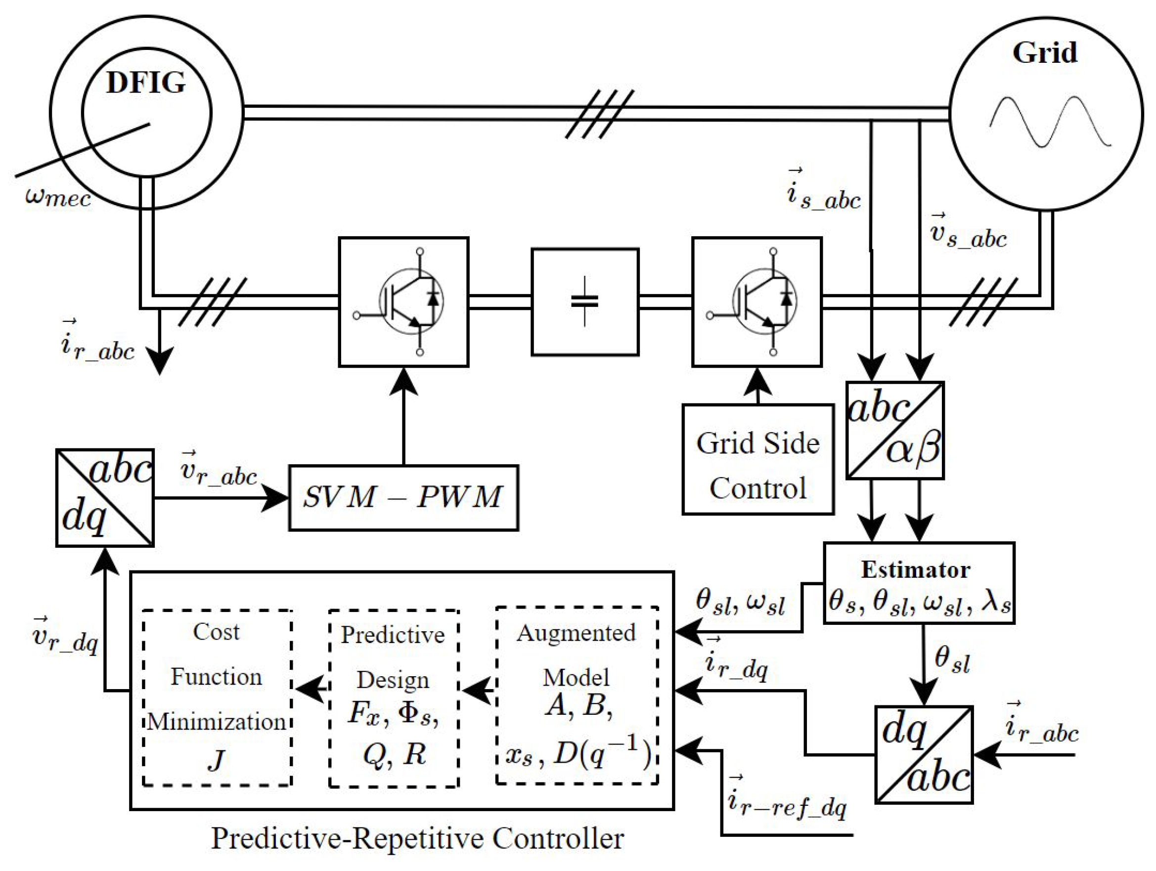
The closed-loop performance of this controller is established by the selection of the weighting matrices $W_x$ and $W_u$. A complete block diagram of the predictive-RC applied to the double-fed induction generator is shown in Figure 1, here are depicted the transformation blocks, the space vector modulation, the proposed PRC, and the estimator, which is similar to the one proposed in [48].

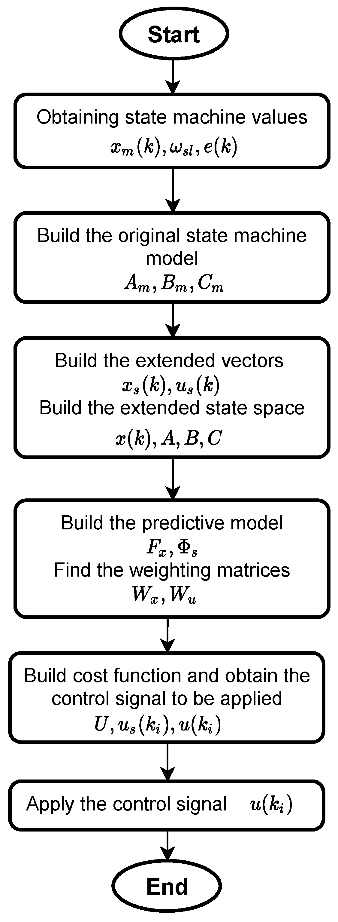
For more details on the control signal generation process, a flowchart of the process from measurement to output of the voltage to be applied is shown in Figure 2.

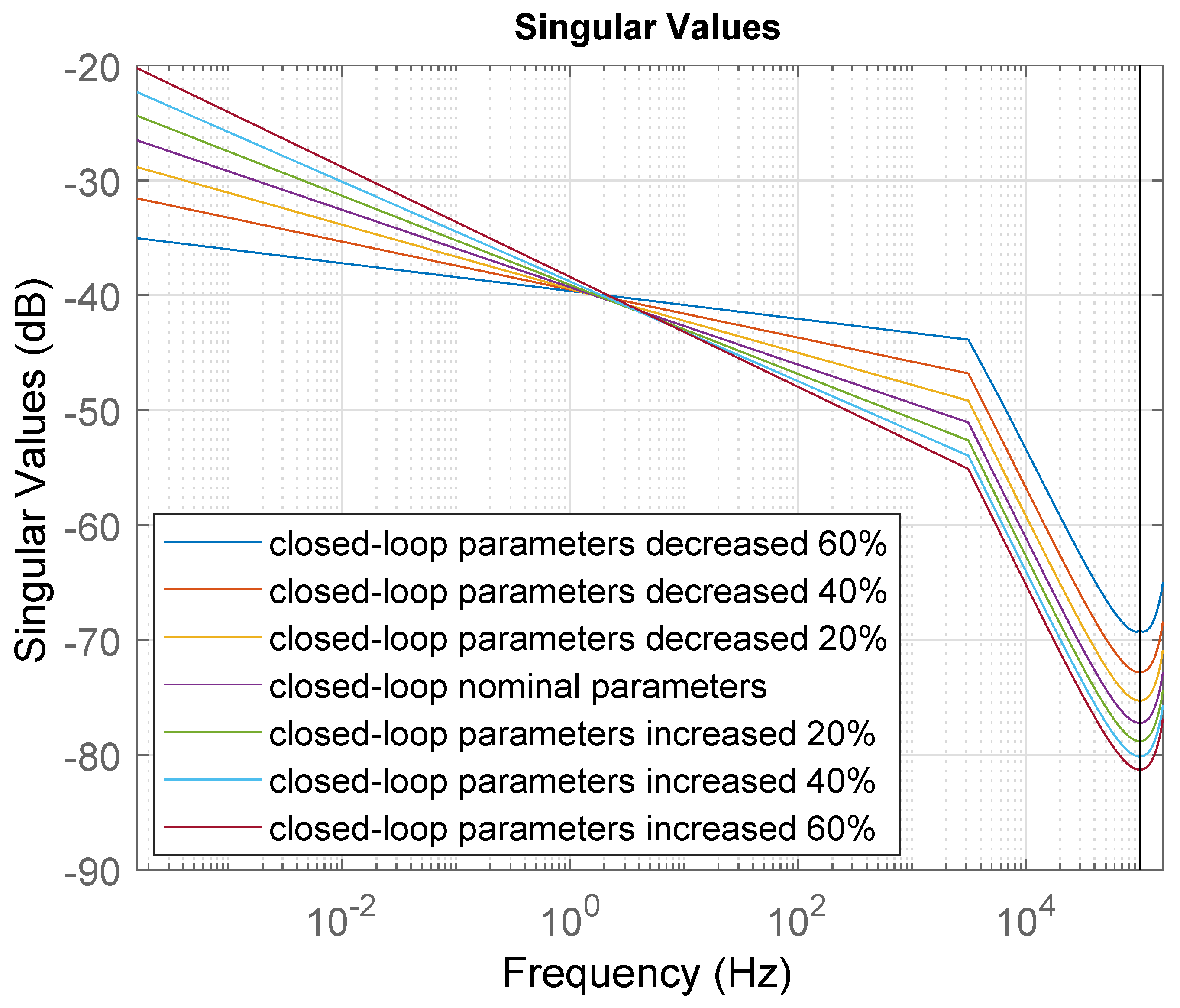
3.2. Controller Stability Due to Parameter Mismatch

To analyze the system model and the controller stability, one of the first points to be considered is the eigenvalues from the state-space model, specifically the eigenvalues of the matrix A. In this DFIG model, the proposed eigenvalues are [0.997 −0.8 0.997 −0.8], and all of them are inside the unitary circle for the discrete system, which means that it has nominal stability in an opened loop. Another important point of analysis in this controller is the stability of itself, which should be analyzed by singular values decomposition, these are determined in order to obtain measurements of robustness and system stability. This is made by means of the state-space model presented above and computing a K matrix using (29) without $x\left(k_i\right)$, which acts as the rotor current and it is considered as a state when is compared with classical state-space feedback.

Singular values can be displayed for the closed-loop system, where it is possible to note that the plant plus the controller are stable considering the theory described in chapter 8 of [49]. Placing the resultant curves in the same figure allows confirming that the system is still stable. This is shown in Figure 3.

4. Experimental Results

Once the controller has been designed, the disturbance model had been embedded and the weighting matrices were set and the experimental implementation for the controller was made up using the general scheme presented in Figure 1. The PRC was implemented using a TMS320F28335 Texas Instruments Digital Signal Processor (DSP). Some electronic boards were used for the voltage $\left(v\right)$ and current $\left(i\right)$ acquisition and an encoder of 3600 p.p.r. to measure rotor speed is also used.

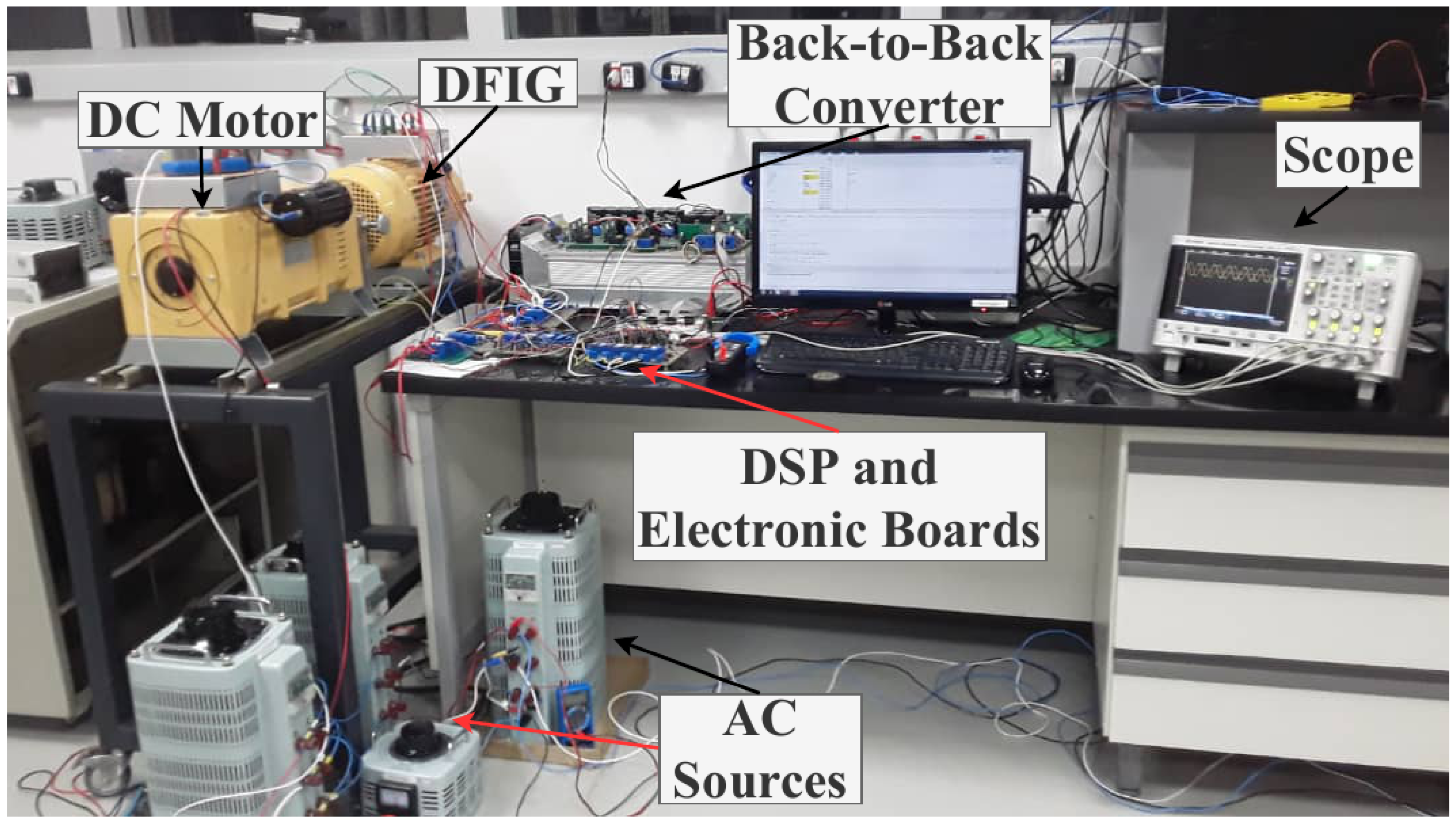
The experimental test bench where all the tests were performed can be seen in Figure 4, it consists of a DC motor that is mechanically coupled to a DFIG to emulate the wind speed, a back-to-back power converter was connected to the DFIG rotor windings and to the stator windings through the grid by means of a set of electrical contactors.

Additionally, the DSP output signals that carry the trigger signals are connected to the power converter and use the space vector modulation (SVM) switching technique at a frequency equal to 10 kHz, which is the same sampling frequency that was chosen for the electric variables. Considering the repetitive characteristic of the proposed PRC, the signal generator polynomial used for this purpose is $D\left(z\right)=1-z^{-1}$. Regarding the predictive characteristics of the controller, the prediction and control horizon were adjusted experimentally with values of $N_p=3$ and $N_c=2$, respectively. The rest of the test bench parameters can be resumed as follows: rated stator voltage $V_{s,n}$ equal to 220/380 $\Delta$–Y, rated stator current $I_{s,n}$ equal to 12 A, and rated power $P_n$ equal to 3 kW. Additionally, the DFIG’s main parameters can be listed as follows: rotor resistance $R_r$ 3.1322 $\Omega$, stator resistance $R_s$ 1 $\Omega$, mutual inductance $L_m$ 0.1917 $\Omega$, stator inductance $L_s$ 0.2010 $\Omega$, rotor inductance $L_r$ 0.2010 $\Omega$, the number of poles is equal to 4, the rated speed is 1800 rpm, rated frequency $f_s$ is 60 Hz, and lumped inertia Constant J is 0.05 kgm². Furthermore, the voltage for the DC link in the back-to-back converter is 130 $V_{dc}$, and the predictive $N_p$ and control $N_c$ horizons for the predictive algorithm are 2 and 3, respectively. The DSP switching frequency is equal to 10 kHz and the signal generator polynomial $D\left(z\right)$ is $1-z^{-1}$.

Wind energy systems can be divided into three control levels [1,50], the first one (Level 1) focuses on the control of the energy on the generator side and the grid side. The second level (Level 2) governs the interaction between the wind turbine mechanical systems and its aerodynamics, this controller generates the MPPT signals that the first level will use as reference signals. The third level (Level 3) aims to handle the integration of the DFIG into the electrical grid and the wind turbine. In that sense, this paper addresses the study of first-level control (Level 1), more specifically the rotor side converter—RSC.

For all the above, this section is split into four subsections, first one summarizes the tests and measurements made from an experiment with constant rotor speed, the second one studies the mismatch parameters of the system, next, the generator behavior during the rotor speed variation is summarized and the last one makes a performance comparison between the proposed PRC with two predictive controllers: a robust FCS controller described in [48] and an MPC-FARE controller based on weighting matrices approach depicted in [45].

4.1. Fixed Rotor Speed Tests

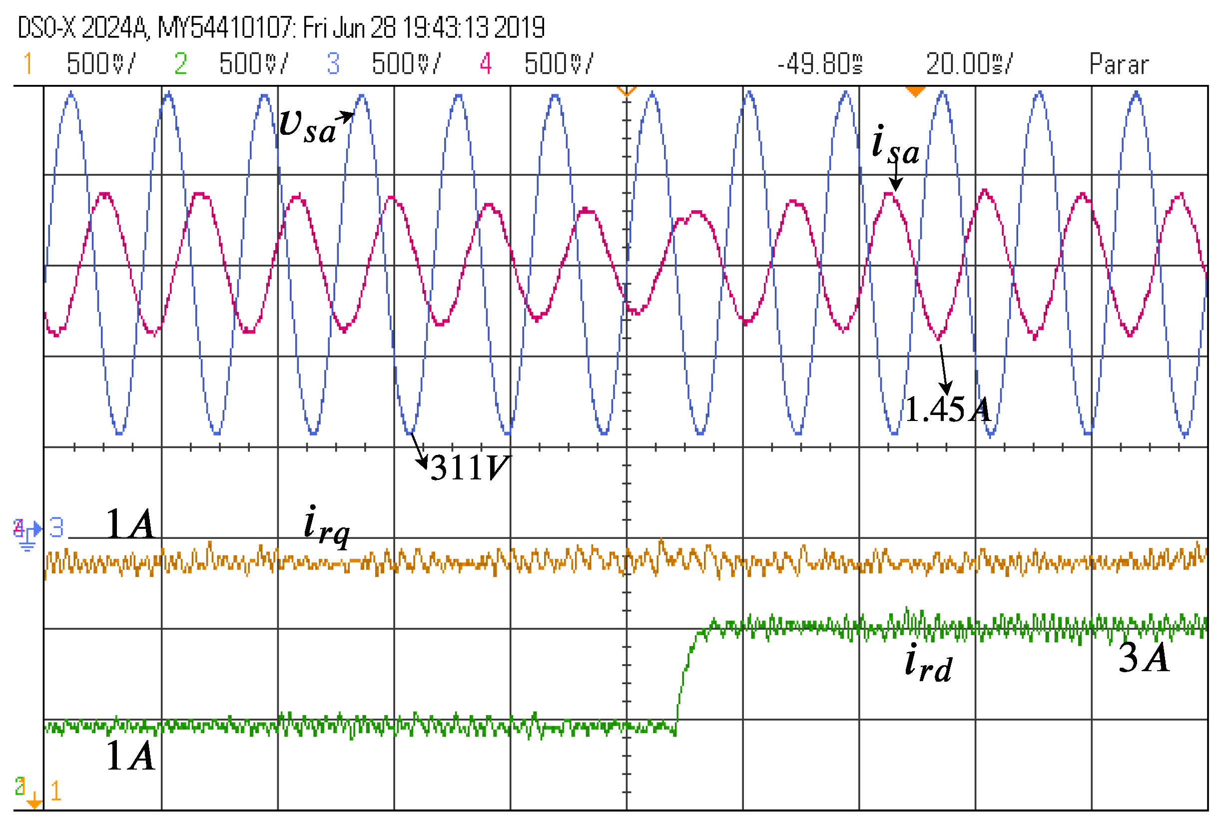
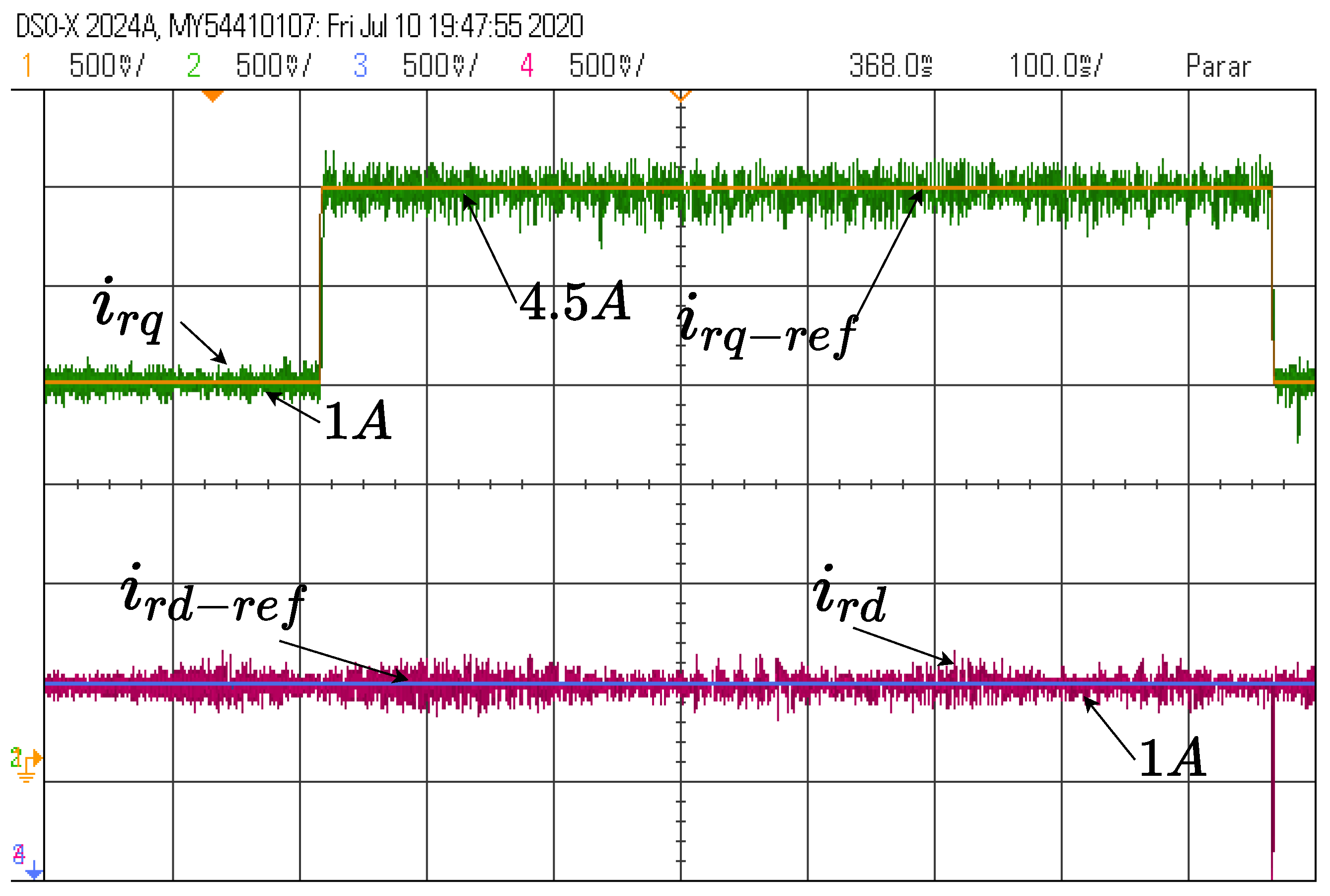
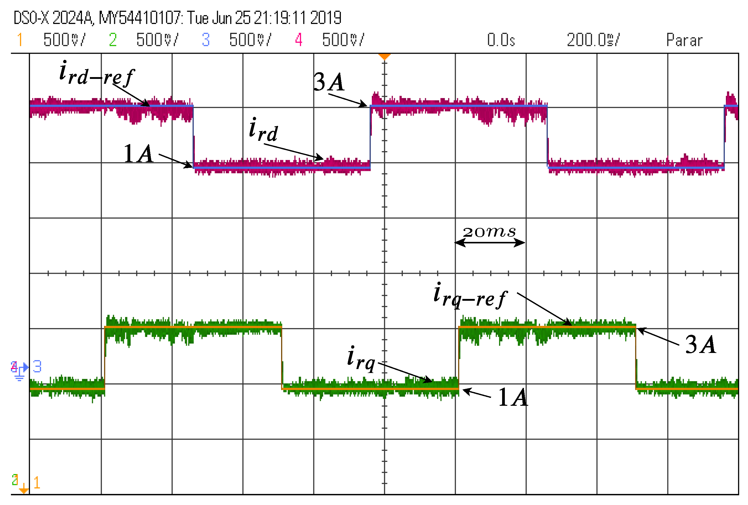
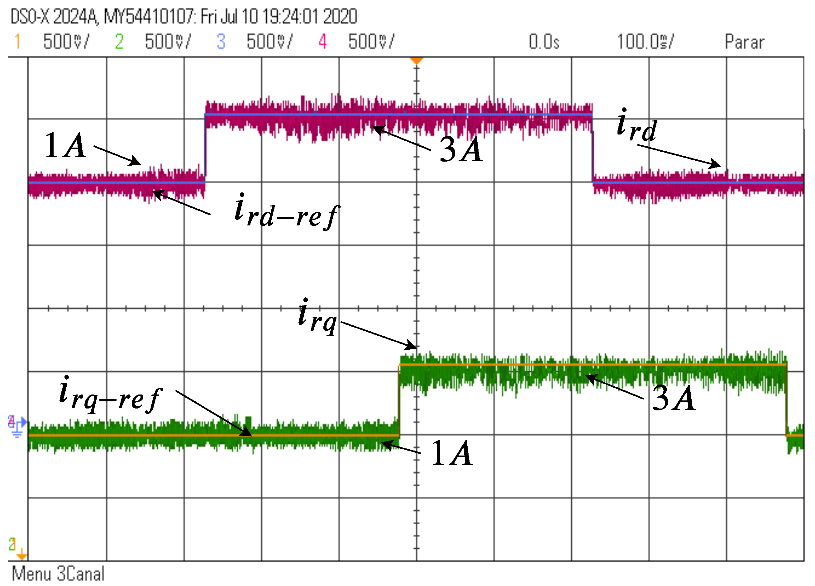
For the first test, a scenario with constant rotor speed equal to $w_m=1750$ rpm was prepared, where the rotor currents ${\overrightarrow{i}}_{rdq}$ (the controlled variables of the PRC) follow its references ${\overrightarrow{i}}_{r-ref\_dq}$ changing its values from 1 A to 3 A and from 3 A to 1 A. These changes in the reference values are not made simultaneously as can be seen in Figure 5. The real rotor currents manage to follow their respective references in an acceptable way. 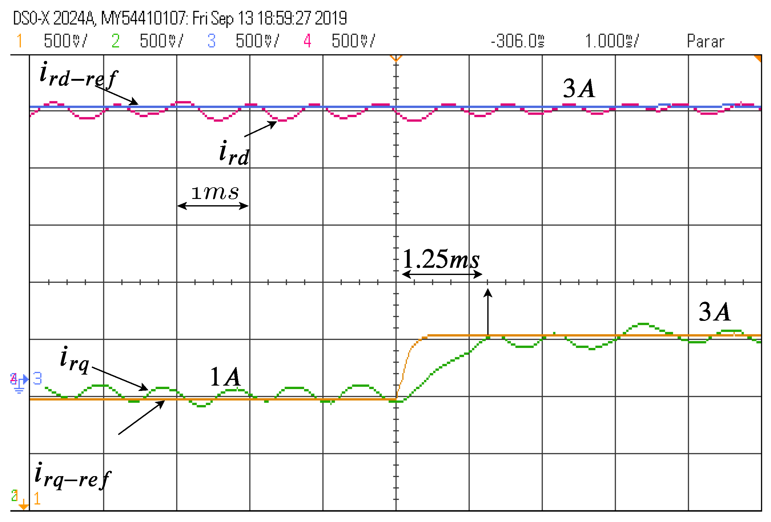Furthermore, Figure 6 presents a detailed view of one rotor current step from 1A to 3A and it can be observed that there is a response without overshoot and a settling time equal to 1.25 ms, approx.

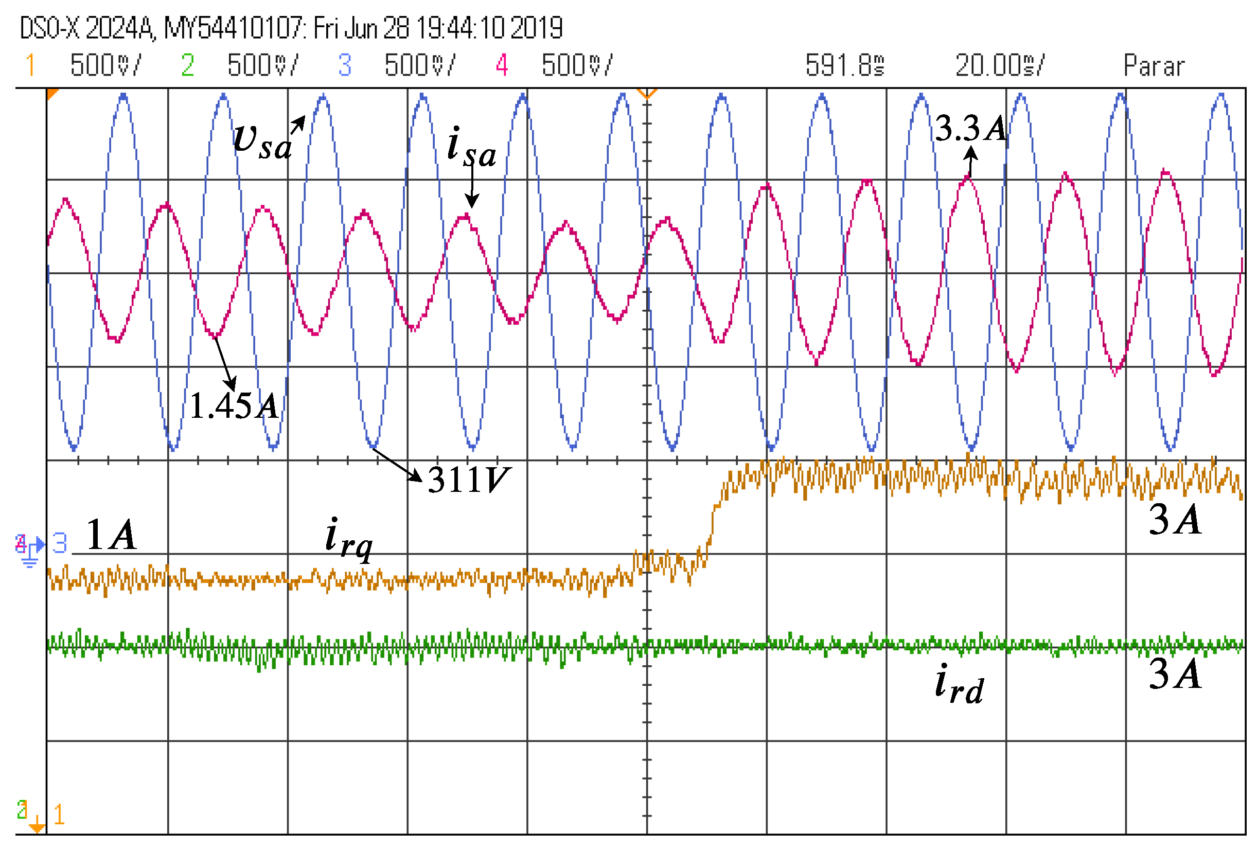
On the other hand, these tests can be analyzed from a different perspective, observing the behavior of other electrical variables while the change in the reference currents is occurring, Figure 7 and Figure 8 show the rotor currents and voltages and stator current for phase A$(v_{sa},i_{sa})$, all this reminding that the reference currents are still changing as is depicted in Figure 5. Specifically, Figure 7 shows the behavior of the stator current while $i_{rq}$ is changing from 1 A to 3 A, while on the left side of the figure the amplitude of the stator current $i_{sa}$ has a value that corresponds to the value of $i_{rq}$ equal to 1 A, an accretion in the value of the rotor current $i_{rq}$ until to 3 A, also increasing, consequently, the amplitude of the stator current.

Analyzing the Figure 8, it can be observed that the rotor current $i_{rd}$ is changing now from 1 A to 3 A, noticing that instead of changing the amplitude of the $i_{sa}$, what is changing now is the phase of this current. Just where the rotor current $i_{rd}$ step change is occurring, an abrupt change in the phase of the stator current $i_{sa}$ can be observed, which is maintained on the right side of the step. The behavior can be inspected in Figure 7 and Figure 8, confirming the theory discussed in [1], according to that, a step change in $i_{rq}$ causes a direct impact on active power $\left(P_s\right)$ and a step change in $i_{dq}$ affects the reactive power $\left(Q_s\right)$, this is: $P_s=-\frac{3}{2}\left(v_s\frac{L_m}{L_s}{i}_{rq}\right)$ and $Q_s=\frac{3}{2}{v}_s\left(\frac{{\psi }_s}{L_s}-\frac{L_m}{L_s}{i}_{rd}\right)$.

In addition to these above tests confirming the controllability of the controller and its performance during fixed rotor speed, other tests were carried out. Figure 9 demonstrates that the controller can perform very well even at different operating points. In this case, Figure 9 shows the controller operating closer to the rated power of the generator with a step change of rotor current $i_{rq}$ from $1A$ to $4.5A$ while $i_{rd}$ remains constant at $1A$.

4.2. Parameter Mismatch Tests

In this section, the same test presented in Figure 5 are reproduced considering $1.5\times R_r$, $1.5\times R_s$ and $1.5\times L_m$ in Figure 10. It can be noticed that the predictive-repetitive controller for DFIG rotor current control reaches the references and the steady state error is minor than 1% while the error in MPC presented in [43,45] is 1.5%.

4.3. Variable Rotor Speed Tests

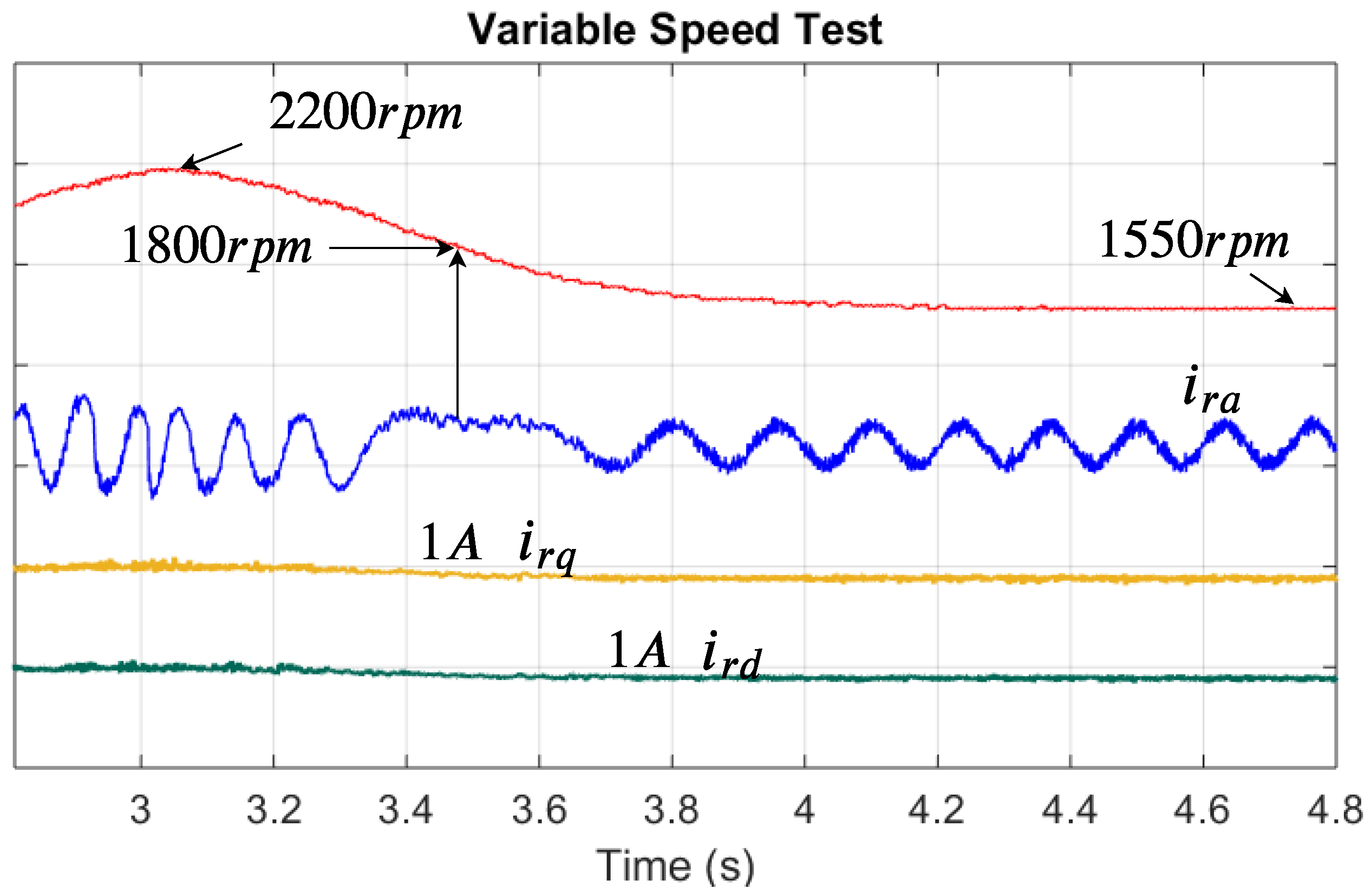
The second test carried out, was the imitation of a wind speed profile, using for that a DC motor mechanically coupled to the DFIG (as is depicted in Figure 4). The mechanical speed increases from a sub-synchronous speed of 1550 rpm, passing by synchronous speed (1800 rpm), up to a super-synchronous top speed of 2200 rpm to finally return to the initial sub-synchronous speed of 1550 rpm. Figure 11 shows the behavior of four variables: the mechanical rotor speed (${\omega }_m$, to show the wind speed profile), the rotor current of the phase A ($i_{ra}$, in the rotor reference frame) and the rotor current components in the dq reference frame $i_{rd},i_{rq}$ (as the controlled variables). Figure 11 shows only the behavior of these four variables when the speed is going down. When this speed falls from 2200 rpm to 1550 rpm, a frequency inversion for phase A of the rotor current at a synchronous speed of 1800 rpm can be observed. This frequency inversion indicates the transition from super-synchronous to sub-synchronous speed and it is proportional to the slip speed ${\omega }_{sl}$.

All of this is happening while the rotor currents $i_{rd}$ and $i_{rq}$ (the controlled variables) remain constant and follow their respective references $(i_{rd-ref}=1A,i_{rq-ref}=1A)$, confirming the proper operation of the PRC proposed here at different mechanical speeds.

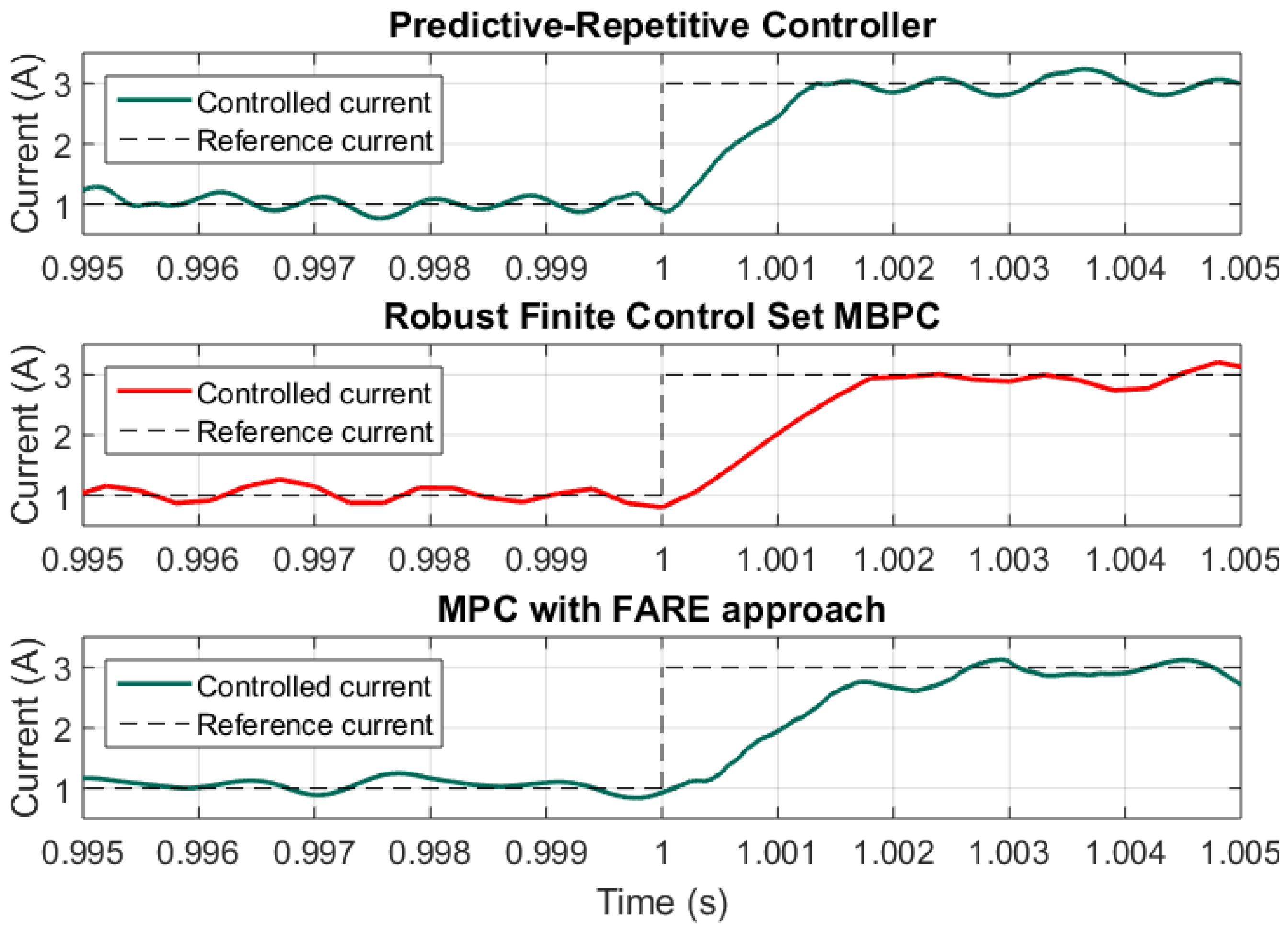
4.4. Controller Performance Comparison

To address the analysis of the proposed controller performance in a deeper way, we used the performance of the robust finite control set [48] and the performance of an MPC with a FARE approach [45] for contrast purposes. All controllers were tuned with the aim of the best reaching for the reference signal, for a more detailed explanation of the controllers tuning methods, there are works such as [45] that have as scope illustrates the tuning process, the results presented here are based on these methods to obtain a fair and easy comparison between controllers. Figure 12 compares the step response of the different strategies. Thus, the comparison was made with a step from 1 A to 3 A. It can be highlighted that the proposed PRC has a better performance due to its settling time being minor at more than 30% when compared with the other approaches. Additionally, the PRC proposed has a lower steady state error when compared with [48] and [45], as is presented in

Table 1. Comparison information between controllers.

Controller	SwF, kHz	SaF, kHz	ST, ms	SSE, %	THDi, %	CB, μs
PRC	10	10	$1.25$	$0.034$	$2.98$	36.2
Robust FCS [48]	-	10	$2.2$	$0.7$	$3.85$	20.3
MPC-FARE [45]	10	10	$2.6$	$1.37$	$5.80$	27.6

.

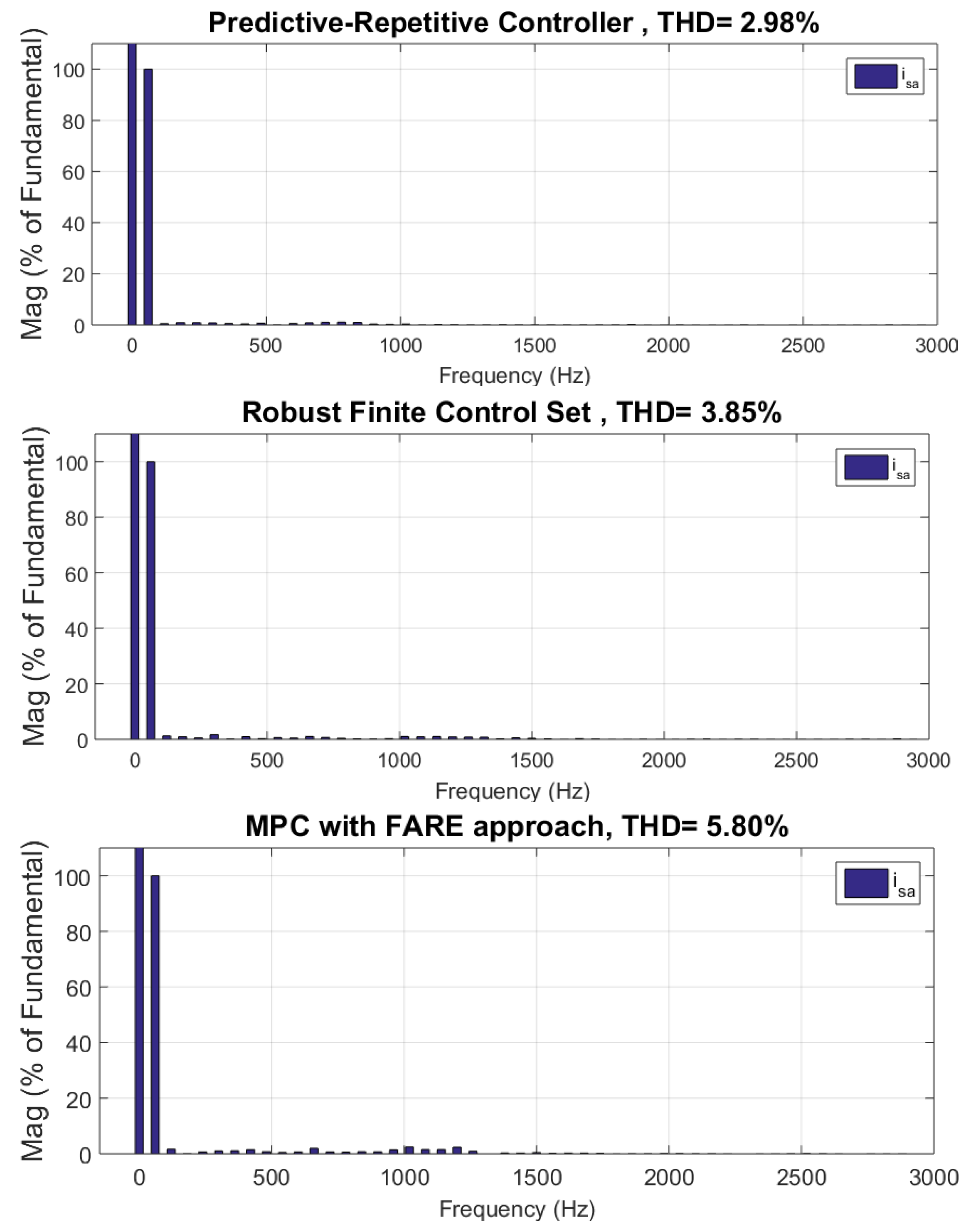
Besides the step response and the settling time, the total harmonic distortion for stator current (THDi) is also an important variable to take into account when the performance of the controllers is evaluated. It is well known that a lower value of the THDi obtains a satisfactory performance of the controller and a minimal THD. Computation of the THDi stator currents for all controllers is compared in Figure 13, at the top of this, appears the PRC, at the middle, the robust finite control set, and at the bottom the MPC with the FARE approach. In all cases, the THDi results in $2.98\%$, $3.85\%$, and $5.80\%$, respectively. Again, the proposed PRC has better performance due to its lower THDi.

Table 1 summarizes all the comparisons between the proposed PRC, the robust finite control set (robust FCS), and the MPC with FARE. Where SwF, SaF, ST, SSE, and CB mean switching frequency, sampling frequency, settling time, steady state error, and computational burden, respectively.

The first point of the comparison present in Table 1 is the switching frequency for the PRC controller and the MPC with the FARE approach the frequency is fixed (due to the fact that both are continuous MPC) and it is equal to 10 kHz for both controllers. However, in the case of the robust FCS, the switching frequency is variable while the sampling frequency is fixed. The authors decided to use the same sampling frequency for all strategies, also based on the frequency limits of the available switching devices. According to [51], the switching frequency of robust FCS is concentrated between $f_s/5$ and $f_s/4$, where $f_s$ is the sample frequency of the controller, that is, between 2 kHz and 2.5 kHz in this case. The results yield other main comparison points, i.e. the PRC is faster in more than $30\%$ of cases against the others, with a lower SSE and better THDi. The lower THDi means that the proposed PRC is better than its contenders in rejection of the switching noise and following the references. As the last check point, the computational burden (CB) of all controllers was compared. In this, the comparison concludes that the proposed PRC is the heaviest one, computationally speaking, the MPC-FARE approach resulted in the middle and FCS is the lightest due to the fact that this is a predictive control that just has to choose between 8 vector options and its prediction horizon is equal to 1.

5. Conclusions

In this paper, a predictive-repetitive controller (PRC) for the DFIG current control was presented. This proposal starts from the use of the traditional and well-known DFIG model based on vector control by stator flux orientation evolving through its model in state-space representation, then, RC characteristics are applied, embedding a signal generator polynomial $D\left(z\right)$ into the state-space model, and thus generating a new expanded state-space model, where the model framework of predictive control will be applied. Additionally, the RC allows increasing the robustness of the controller against parameter mismatch.

The PRC was implemented in the experimental test bench as is shown in Figure 4, with the parameters described in Section 4. During the test developed at fixed rotor speed, the experimental results yielded a good reference tracking and fast step response, confirming the rotor currents control and hence the power control of the DFIG. In the variable rotor speed test, it was possible to observe the behavior of system variables and their controllability under sub-synchronous, synchronous, and super synchronous speeds. In summary, this PRC reached the expectation according to its fast response, low THDi, and low steady-state error, demonstrating that can be a real alternative for the DFIG control in wind energy applications.