A Day-Ahead Energy Management for Multi MicroGrid System to Optimize the Energy Storage Charge and Grid Dependency—A Comparative Analysis

Abstract

Microgrid (MG) is a combination of distributed generators (DGs), energy storage systems (ESSs), and loads connected to distribution network that can either be in islanded mode or grid-tied mode. Similarly, a multi-microgrid (MMG) system is a number of interconnected MGs connected with a larger and complex distribution network. Recently, the MMG energy management has created new challenges due to the inherent intermittency, uncertainty, and probabilistic nature of renewable based DGs output and varying load demands. To ensure the efficient operation and optimal energy management in the MMGs, this work proposes a two-stage, a day-ahead, simultaneous energy management strategy (EMS) of the MMG system as well as the MG system. At the first stage, each MG assumes a day-ahead predicted load demand and DGs output. At the second stage, through EMS, the energy scheduling, minimization of the main grid dependency, and maximization of the stored energy in the ESS are managed simultaneously. Four case studies are considered with four interconnected MGs with different DGs output and different initial state of charge (SOC) of ESS along with varying load demand. The proposed optimization model is formulated in the standard form using MATLAB OptimProblem, and compared with heuristic state flow-based EMS. Results show that the total grid dependency will be reduced to zero and ESS depth of discharge (DoD) will be increased up to 50% with the proposed optimization model.

1. Introduction

Distributed energy resources (DERs), e.g., PV arrays and wind turbines, are becoming the main component of future power system, to ensure system sustainability and reduce fossil fuel-based power generation [1,2]. DERs are also very useful to supply power to the areas with remote or no access to the main grid or areas, with no transmission and distribution infrastructure [3,4]. However, renewable energy systems (RESs) also introduce challenges like intermittency in power generation, creating discontinuity in transmission and load distribution. In recent years, the integration of energy storage systems (ESSs) has been substantially increased to overcome this challenge [5]. Another solution to this challenge is the emergence of microgrids (MG) to integrate DERs with ESSs and loads, and form an independent low voltage, islanded, or grid-connected network [6], as shown in Figure 1. In grid-connected mode, an MG should provide a bi-directional power flow to connect to a distribution network, while in islanded mode, the EMS manages to supply the DER power output to the MG load, and store it in the ESSs [7].

Figure 1. A schematic diagram of a microgrid.

To take advantage of the bi-directional power flow, a new concept of multi-microgrid (MMG) system has emerged to allow for the interaction of neighboring MGs [8,9], as shown in Figure 2. In terms of topology, the MMG systems are categorized into two frameworks, i.e., centralized and distributed. In the centralized topology, the EMS is easy to design and implement; however, it suffers from high computational complexity, longer communication distance, communication delay, and lower reliability [10]. In the distributed framework, each MG in the MMG network is managed by a local EMS, interacting with the neighboring MG using global EMS to achieve a similar objective [11]. If we increase the number of MGs in the MMG distribution network, the MG scheduling becomes a challenge due to inherent uncertainties of power system, load demand, and RESs output power. To overcome this problem and enhance the efficiency of a MMG system, several studies are done by different researchers [12,13,14]. A dynamic pricing scheme was proposed for a home energy management system to obtain an economic benefit [15]. In [16], an optimization problem is proposed for the maximum utilization of the solar PV system through battery charging. In [17], a problem is formulated for minimizing the purchasing power from a conventional grid. In [18], a standalone system is presented and a methodology is proposed to find an optimal system sizing for household electrical appliances, considering the system cost. In [19], a similar work for Optimal planning and design of low-voltage, low-power solar DC microgrids for the selected cities in India is presented. In [20], an optimization approach is proposed to minimize the power flow between the solar PV system, ESSs, and grid with the main objective of minimizing the net cost of ESS charging.

Figure 2. A schematic diagram of interconnected multi-microgrid system.

A dynamic optimization model is presented for power sharing among DERs without considering battery degradation cost to increase battery lifetime in [21]. In [22], for an ESS in an islanded MG system, a non-optimal model is proposed to ensure state of charge (SOC) staying above a threshold level. A method is proposed in [23] to decompose a global optimization problem into local sub-problems, and solve each sub-problem to achieve the global optimal solution. Zhang et al. [24] investigate whether the Shared-ESS can assist energy savings for multiple users through Peer-to-Peer (P2P) trading. Moreover, with the increasing number of market participants in the integrated energy system, a benefit allocation scheme is necessary, ensuring reasonable benefits for every user in the network. In [25], a demand-side management methodology is proposed to improve the household load for estimating power production by the MG. Xiao et al. [26] proposes a stochastic optimization model for generating the optimal price-maker trading strategy for a wind power producer using virtual bidding, which is a kind of financial tool available in most electricity markets of the United States. In [27], a heuristic model is presented to find an optimal EV charging in the time management system. In [28], a heuristic state flow based multi-agent methodology for MG EMS is discussed. In [29], a two-stage energy management strategy for minimizing the consumer energy cost and flattening the load profile is proposed. Other research on energy management of MMG with multi-agent structures is also published in [30,31]. Despite a great deal of research in the area of microgrids, the proposal for the development of an energy management strategy for an MMG system is still missing, where each MG simultaneously manages different types of DGs and ESSs with varying demand responses. In fact, the possible issues due to the varying demand responses, different DG types, and different ESS scenarios have not yet been covered and discussed. Considering the probabilistic nature of all DGs and load demand, a day-ahead planning strategy to perform an optimized energy management for the MMG system seems necessary. In short, we believe the previous research works have not addressed the following critical problems:

• optimal energy scheduling in management of interconnected MMGs system,
• consideration of the energy management of the local MGs while scheduling for MMG,
• a mechanism for energy exchange between different MGs in the same distribution network,
• depth of discharge (DoD) for ESSs to maintain battery health while also reducing the main grid dependency.

Considering the above critical problems, this paper addresses and proposes a day-ahead optimal energy management strategy to maintain the depth of discharge (DoD) of each ESSs and to reduce the grid dependency with neighborhood sharing. The main contributions of this paper are briefed as follows:

• A two-level optimization strategy is proposed. Each local EMS optimizes the energy scheduling of it’s MG and then exchanges a small amount of information with its neighboring MG’s EMSs to collectively optimizes the energy scheduling of the MMG system.
• An optimization model is formulated in the standard form for energy management of the MMG system considering all DGs, ESSs, and load connected with the distribution network.
• Unlike heuristic state flow-based strategy, ‘a day-ahead’ optimization strategy for energy management of an MMG system is proposed.
• The proposed optimization model provides a plug and play option to readily extend the MMG network.

The subsequent sections of this paper are described as follows. In Section 2, a system model formulation is presented. Section 3 explains heuristic state flow-based strategy for EMS. In Section 4, the proposed optimization-based strategy for energy management is proposed. Case studies and system specification are briefly discussed in in Section 5. In Section 6, various case studies are presented in order to compare the proposed model with the heuristic approach in terms of power balance, maintaining the DoD of ESS and reducing the dependency on the main grid. The paper concludes in Section 7.

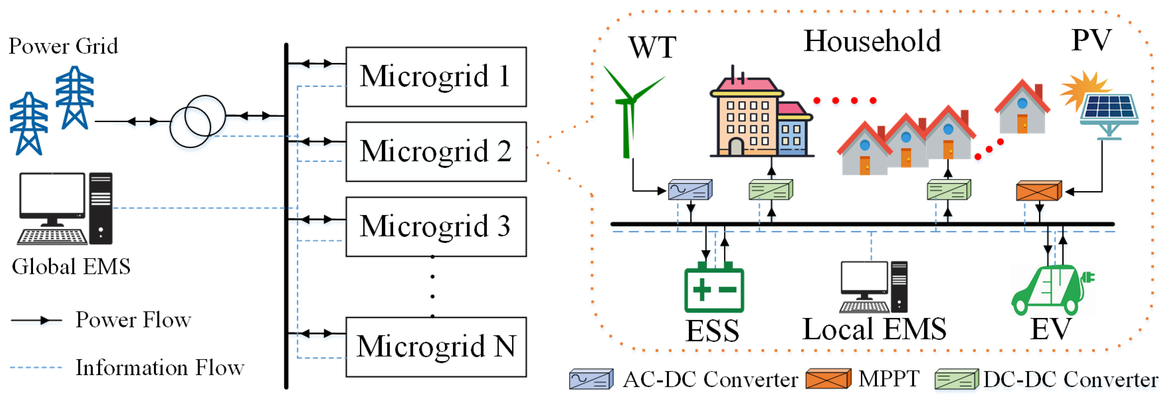
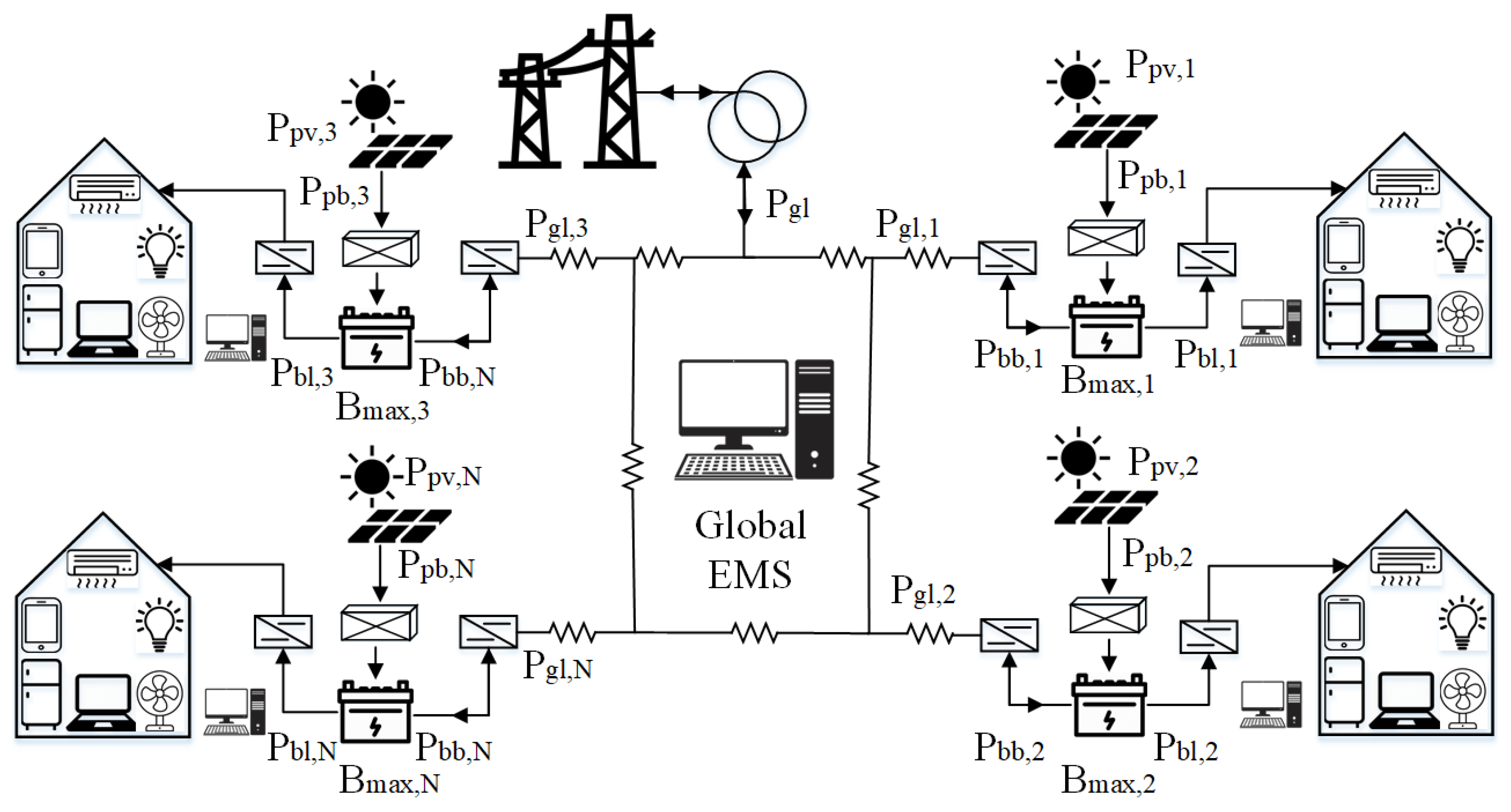
2. System Model Formulation

In order to design a system model, it is important to analyze the system in terms of its parameters such as the load requirements, available DGs, and ESSs of each MG as well as neighboring MGs. In this section, we will study all the individual system’s components. The output power of a PV DG mainly depends on incident irradiance and temperature. In [32,33], a mathematical model to quantify PV output and temperature losses is presented and is given by

$$P\left(t\right)=A\times {\eta }_{pv}\times I_{rr}^t\left(t\right),\forall t,$$

(1)

where ${\eta }_{pv}$ is PV panel efficiency, A represents the system size, and $I_{rr}^t\left(t\right)$ represents the temperature compensated irradiance and is given by [34]:

$$I_{rr}^t\left(t\right)=(1-(T_{cell}\left(t\right)-25)\times 0.0045)\times I_{rr}\left(t\right),\forall t$$

(2)

$$T_{cell}\left(t\right)=T_{amb}\left(t\right)+(0.01875\times I_{rr}\left(t\right)),\forall t$$

(3)

where $T_{cell}\left(t\right)$ and $T_{amb}\left(t\right)$ are cell temperature and ambient temperature, respectively. Similarly, $I_{rr}\left(t\right))$ represents the incidence irradiance, which shows a direct relation between cell temperature and incidence irradiance. Therefore, with inclusion of temperature losses, the power produced by the $i^{th}$ MG for a complete cycle of a day is given by (4):

$$P_{pv}^i=\left[P_{pv}^i\left(1\right),P_{pv}^i\left(2\right),\cdots ,P_{pv}^i\left(T\right)\right],\forall i$$

(4)

The load of an individual MG mainly depends on the number of users in each MG and their respective load demands as per their requirements. Therefore, the load of $i^{th}$ MG for a complete cycle of the day can be given by

$$P_{load}^i=\left[P_{load}^i\left(1\right),P_{load}^i\left(2\right),\cdots ,P_{load}^i\left(T\right)\right],\forall i$$

(5)

Similarly, each MG may have an ESS with its charging and discharging rates depending on manufacturer technology as given by

$$B_{ava}^i=\left[B_{ava}^i\left(1\right),B_{ava}^i\left(2\right),\cdots ,B_{ava}^i\left(T\right)\right],\forall i$$

(6)

$$B_c^i\left(t\right)<=ChargeRate,B_d^i\left(t\right)<=DischargeRate,\forall i,t$$

(7)

Further, each ESS has initial and final state of charge given by

$$B^i\left(0\right)=B_{initial}^i,B^i\left(T\right)=B_{final}^i,\forall i$$

(8)

Since the battery life depends on the DoD, the charge level of the battery at any time t cannot be below/above its minimum/maximum allowed charge level as given by

$$B_{ava}^i\left(t\right)>=B_{min}^i,B_{ava}^i\left(t\right)<=B_{max}^i\forall i,t$$

(9)

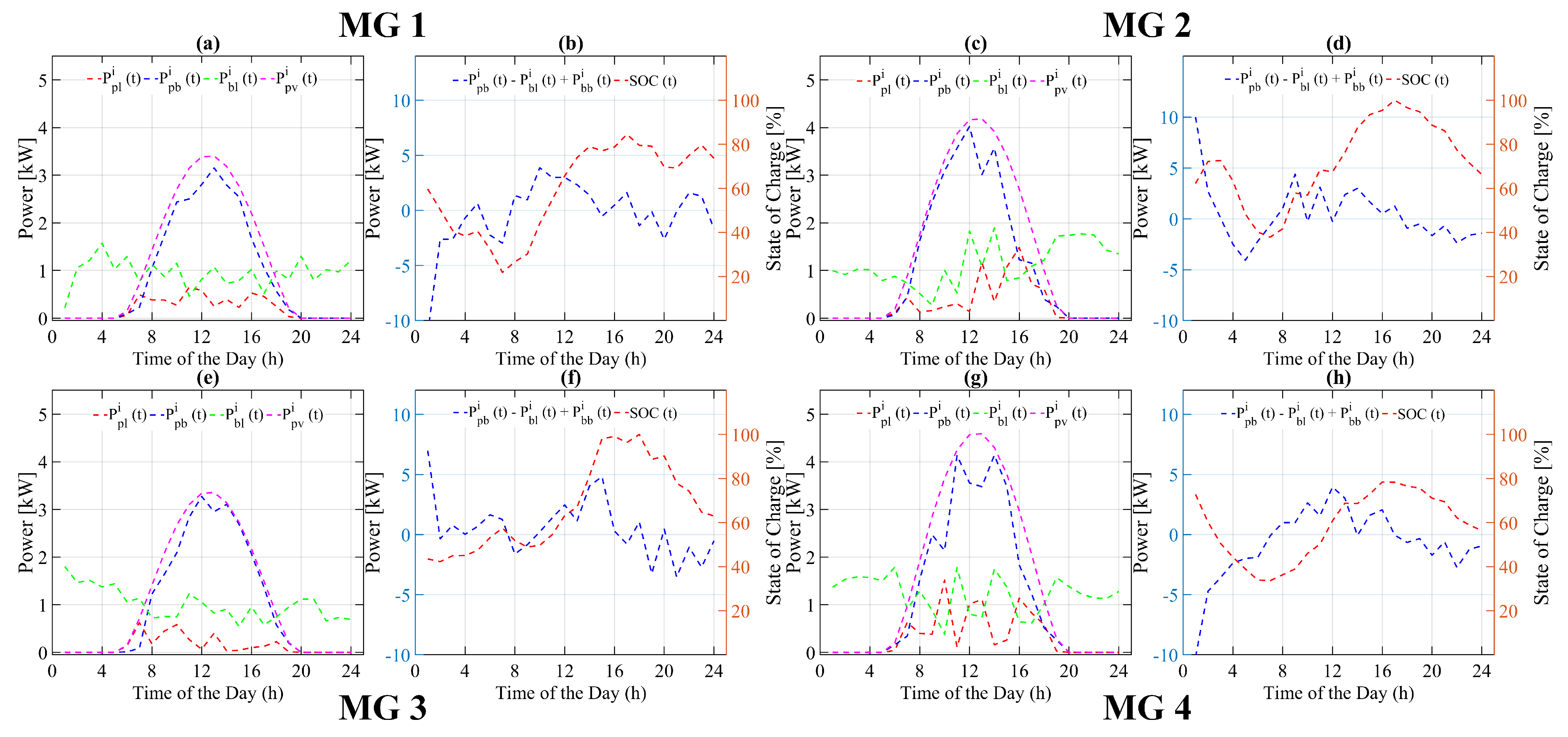
3. The Heuristic State Flow Based Strategy for Energy Management

In heuristic state flow based strategy, the current value of all system’s components such as DGs output, available ESS charge, and load is considered. It does not consider the past and future values of any system component. The power-flow and charging/discharging algorithms for PV and ESS are developed to satisfy the load requirements. At t = 1 and n = 1, the surplus and insufficient power of PV can be calculated by

$$P_{pv,rem}^i\left(t\right)=P_{pv}^i\left(t\right)-P_{load}^i\left(t\right),\forall i,t,$$

(10)

where $P_{pv}^i\left(t\right)$, $P_{load}^i\left(t\right)$ and $P_{pv,rem}^i\left(t\right)$ represent the available PV power, load demand, and remaining power after satisfying the load of ith MG at time t, respectively. $P_{rem}^i\left(t\right)$ in (10) being greater than zero indicates some surplus power at the PV end, and below zero indicates insufficient power to meet load demand. In the former case, the remaining PV power will go to ESS to charge the battery as given by

$$B_{}^i\left(t\right)=B_{}^i(t-1)+P_{pv,rem}^i\left(t\right),\forall i,t$$

(11)

where $B_{}^i\left(t\right)$ is the state of charge of ith battery at time t. In the latter case, the load is powered with available storage as given by

$$B_{}^i\left(t\right)=B_{}^i(t-1)-P_{load}^i\left(t\right),\forall i,t$$

(12)

$B_{}^i\left(t\right)$ is the state of charge (SOC) of ith battery at time t in (12) greater than zero, which means some surplus power at the battery end, whereas lower than zero means the battery has insufficient power to meet load demand at time t.

In the former case, Equation (12) will remain valid and unchanged, while in later cases, the Equation (12) will not remain valid to satisfy load demand. Therefore, the ESS should receive power from its neighboring MG ESS. If the neighboring MG also has insufficient power, then it will check the next neighboring MG (n = n + 1) and it will continue until the Nth MG. So, the ESS charging/discharging as given in Equations (11) and (12) will be modified and are now given by

$$B_{}^i\left(t\right)=B_{}^i(t-1)+P_{pv,rem}^i\left(t\right)+\sum _{i=1}^{N}b{b}_c^i\left(t\right),\forall i,t,$$

(13)

$$B_{}^i\left(t\right)=B_{}^i(t-1)-P_{load}^i\left(t\right)-\sum _{i=1}^{N}b{b}_d^i\left(t\right),\forall i,t,$$

(14)

where $b{b}_c^i\left(t\right)$ and $b{b}_d^i\left(t\right)$ are charging and discharging power flow between ESSs of neighboring MGs. After combining both charging and discharging Equations (13) and (14), the state of charge of ith battery at time t is given by (15):

$$B_{}^i\left(t\right)=B_{}^i(t-1)+P_{pv,rem}^i\left(t\right)-P_{load}^i\left(t\right)+/-\sum _{i=1}^{N}b{b}_{c/d}^i\left(t\right),\forall i,t$$

(15)

If $P_{pv}^i\left(t\right)$ and $B_{}^i\left(t\right)$ is still less than zero, then the load demand will be satisfied with power from the main grid. The power required from the main grid for load can be given by

$$P_G^i\left(t\right)=P_{load}^i\left(t\right)-P_{pv}^i\left(t\right)-P_{ESS}^i\left(t\right),\forall i,t$$

(16)

If $B_{}^i\left(t\right)$ is greater than zero and reaches $B_{max}^i$, then the excess power from ESS is delivered to the main grid and is calculated by

$$P_G^i\left(t\right)=B_{}^i\left(t\right)-B_{max}^i,\forall i,t$$

(17)

After satisfying the load demand and all constraints of MG at n = 1 and t = 0, the state flow model steps forward to the next MG at n = n + 1 and t = 0 and repeats the same steps until n = N. After completing the same steps at n = N and t = 0, the state flow model will repeat same procedure with t = t + 1 until t = T.

All steps of the heuristic state flow based energy management strategy discussed above are also presented in Figure 3.

Figure 3. The steps of the heuristic state flow based energy management strategy.

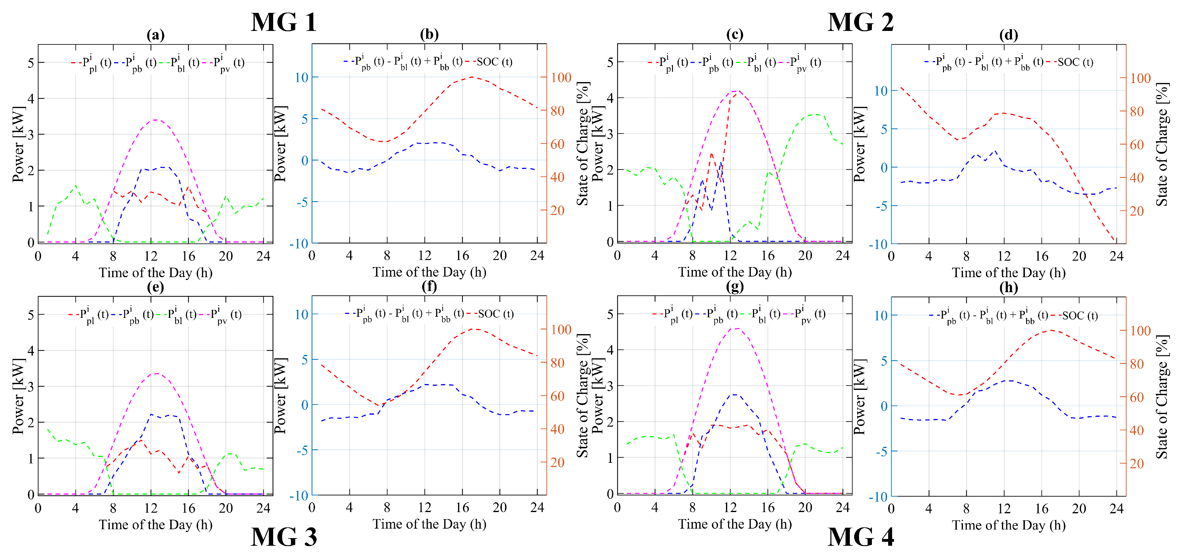
4. The Proposed Optimization Based Strategy for Energy Management

In this section, we propose an optimization based strategy for energy management and the associated objective functions and system constraints. In our proposed strategy, the overall objective function is to minimize the grid dependency in energy management and to maximize the stored energy in the ESSs while satisfying all system constraints for a complete cycle of the day.

4.1. Objective Function

The objective function can be given as

$${\displaystyle \underset{\left(P_{pl}^i,P_{pb}^i,P_{gl}^i,P_{gb}^i,P_{bl}^i,B^i,P_{bb,c}^i,P_{bb,d}^i\right)}{min}\sum _{t=1}^T\sum _{i=1}^N{G}_i\left(t\right),\forall i,}$$

(18)

where $P_{pl}^i$, $P_{pb}^i$, $P_{gl}^i$, $P_{gb}^i$, $P_{bl}^i$, $P_{bb}^i$, and $B^i$ are different power flows between PV, ESS, load, and the main grid of $i^{th}$ MG, respectively. Each system component has lower and upper bounds called system constraints, and is divided into inequality and equality constraints.

4.2. Inequality System’s Constraints

There are some non-negativity inequality constraints on energy flow between different DERs and loads as given by

$$\mathrm{Power}\mathrm{transfer}\mathrm{from}\mathrm{PV}\mathrm{to}\mathrm{load}:P_{pl}^i\left(t\right)⩾0,\forall i,t$$

(19)

$$\mathrm{Power}\mathrm{transfer}\mathrm{from}\mathrm{PV}\mathrm{to}\mathrm{battery}:P_{pb}^i\left(t\right)⩾0,\forall i,t$$

(20)

$$\mathrm{Power}\mathrm{transfer}\mathrm{from}\mathrm{battery}\mathrm{to}\mathrm{load}:P_{bl}^i\left(t\right)⩾0,\forall i,t$$

(21)

$$\mathrm{Power}\mathrm{transfer}\mathrm{from}\mathrm{main}\mathrm{grid}\mathrm{to}\mathrm{load}:P_{gl}^i\left(t\right)⩾0,\forall i,t$$

(22)

$$\mathrm{Power}\mathrm{transfer}\mathrm{from}\mathrm{main}\mathrm{grid}\mathrm{to}\mathrm{battery}:P_{gb}^i\left(t\right)⩾0,\forall i,t$$

(23)

As mentioned, the battery energy density is generally restricted by the minimum and the maximum limits as defined by the following inequality constraint

$$B_{max}^i⩾B^i\left(t\right)⩾B_{min}^i,\forall i,t$$

(24)

Similarly, the charging and discharging rate of the battery is also restricted by allowable limits. Therefore, the inequality constraints on battery charging and discharging rate are given by

$$P_{c,rate,min}^i⩽\sum _{j=1}^N{P}_{bb,c}^i⩽P_{c,rate,max}^i,\forall i,t,$$

(25)

$$P_{d,rate,min}^i⩽\sum _{j=1}^N{P}_{bb,d}^i⩽P_{d,rate,max}^i,\forall i,t,$$

(26)

where $P_{c,rate,max}^i$ and $P_{c,rate,min}^i$ are the minimum and maximum charging rate of the ith battery, respectively. Similarly, $P_{d,rate,max}^i$ and $P_{d,rate,min}^i$ are the minimum and maximum discharging rate of ith battery, respectively.

4.3. Equality Constraints

There are also some equality constraints on DGs output, ESSs, and load demand. The load demand must be fulfilled either by the DGs output, available ESS, or the main grid. Therefore, the equality constraint on the load demand is given by

$$P_{pl}^i\left(t\right)+P_{bl}^i\left(t\right)+P_{gl}^i\left(t\right)=P_{load}^i\left(t\right),\forall i,t,$$

(27)

where $P_{load}^i\left(t\right)$ is the load demand of ith MG at time t. Similarly, the output of DGs can either be supplied to the load or to charge the ESS. Therefore, the equality constraint on DGs output is given by

$$P_{pl}^i\left(t\right)+P_{pb}^i\left(t\right)=P_{pv}^i\left(t\right),\forall i,t,$$

(28)

where $P_{pv}^i\left(t\right)$ is the generation of ith MG at any time t. The simultaneous charging and discharging of the battery and the resultant $SOC$ of the ith battery is given by

$$\begin{array}{c}\hfill B^i(t+1)=B^i\left(t\right)+P_{gb}^i\left(t\right)-P_{bl}^i\left(t\right)+\sum _{j=1}^N{P}_{bb,c}^i\\ \hfill -\sum _{i=1}^N{P}_{bb,d}^i,\forall i,t,\end{array}$$

(29)

where $P_{gb}^i$ and $P_{bl}^i$ are the power flow between DG, ESS, and the load of ith MG, respectively, and $B^i\left(t\right)$ and $B^i(t+1)$ are the available energy in ES of ith MG at time t and $t+1$, respectively. Similarly, the $P_{bb,c}^i$ and $E_{bb,d}^i$ are the charging and discharging power of ith ESS, respectively. The initial and final energy state of the ESS is also restricted by the system defined value of B, and is given by

$$B^i(t=1)=B_{initial}^i,\forall i$$

(30)

$$B^i(t=T)=B_{final}^i,\forall i$$

(31)

The defined objective function in Equation (18), along with all inequality and equality constraints Equations (19)–(31), for all power flows as shown in Figure 4, is formulated in the standard form of optimization using OptimProblem available in MATLAB 2020.

Figure 4. A schematic diagram of interconnected multi-microgrid system showing power flow between different DERs and ESSs.

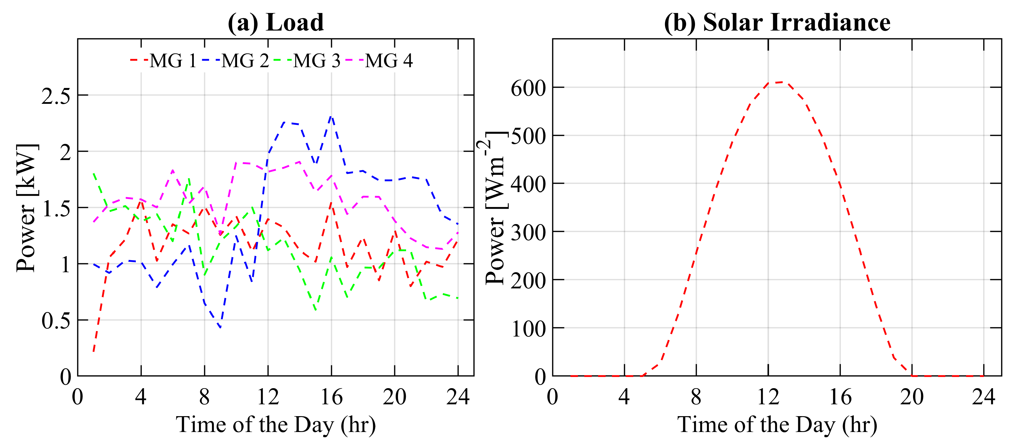
5. Case Studies and System Specifications

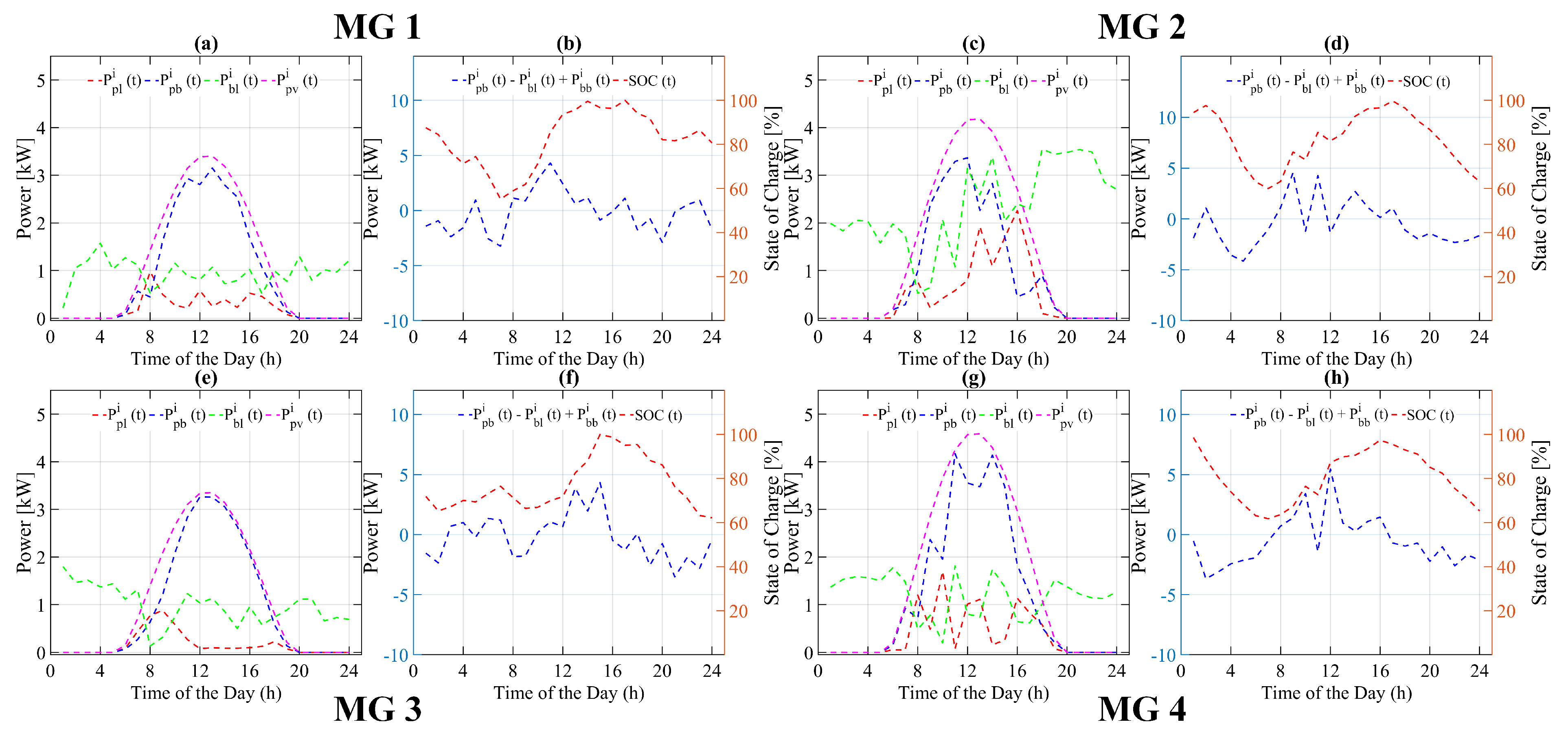
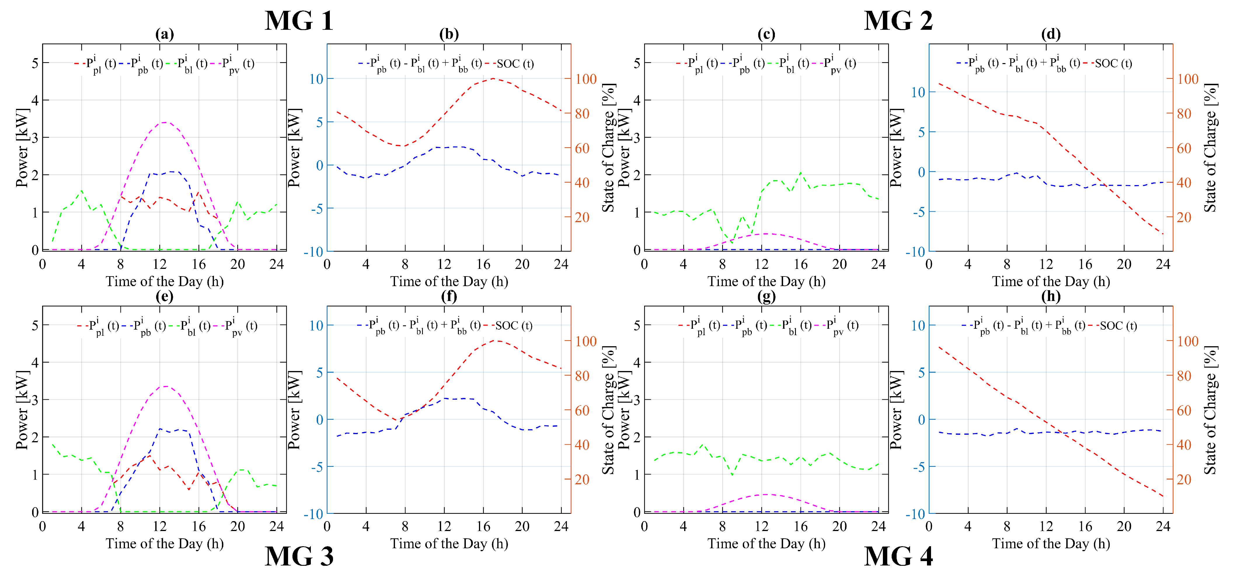
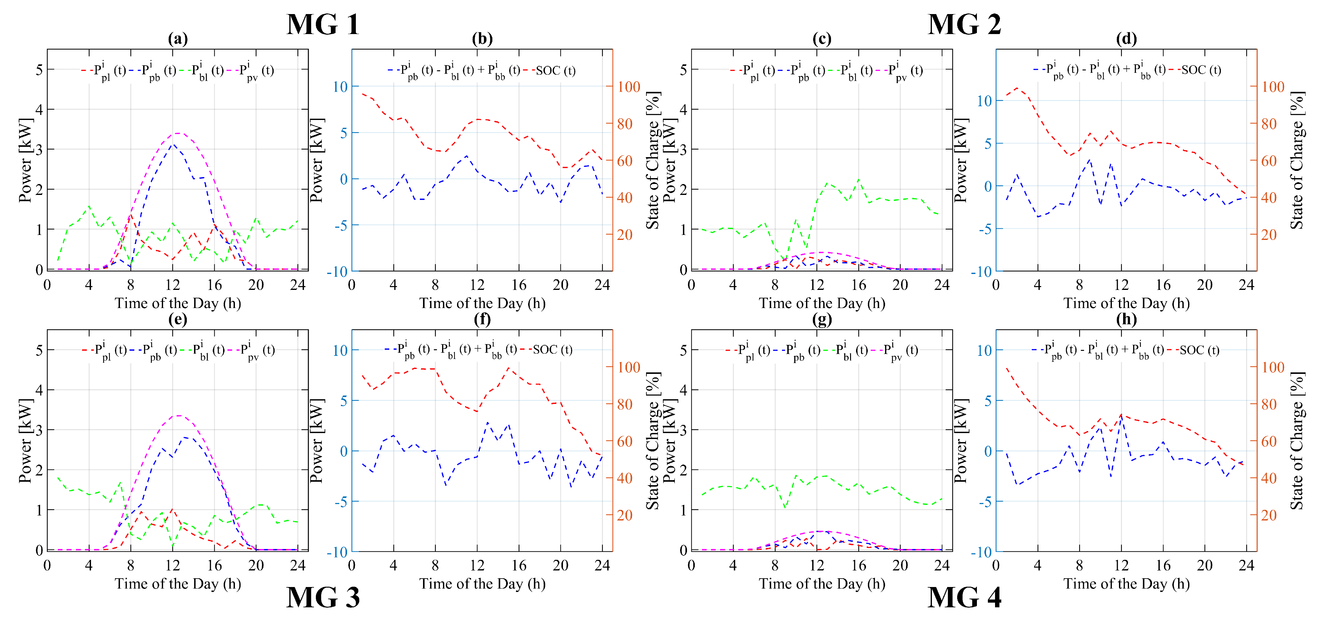
In this section, we have presented the system parameters and case studies. The number of MGs in the study can be considered as N; however, for simplicity we consider N as 4. As the changes in MG load and generation profile are instantaneous, time resolution should be minimized. For our presented work, the time resolution t is 1 h to lower the computational burden. The distribution voltage is considered to be 48 V. The solar irradiance data is adopted from the online available source, the National Solar Radiation Database (NSRDB), for a given location [35]. The NSRDB is a serially complete collection of hourly and half-hourly values of meteorological data and the three most common measurements of solar radiation: global horizontal, direct normal, and diffuse horizontal irradiance. The peak sunlight hour (PSH) for a given location is 4.97 per day, while the hourly incidence irradiance of a given location is also presented in Figure 5b. The load profile is adopted from the Pakistan Residential Electricity Consumption Dataset (PRECON) [36]. PRECON is a first of its kind extensive dataset of electricity consumption patterns of users in developing countries. The dataset has been collected through smart meters over a period of one year. The cumulative load of each MG is given in Table 1 and the hourly load of each MG is also presented in Figure 5a. Depending on the load profile, each MG has been installed with a varying PV and ESS size. All system parameters are shown in Table 1.

Figure 5. (a) Varying load demand of all microgrid under normal day condition, (b) Solar irradiance data used for simulation fro a complete cycle of day [35].

Table 1. The detail of system parameters.

System Parameters	Value (Unit)
No. of microgrids	4
Peak Sunlight hour	4.97
Distribution Voltage	48 (V)
Maximum SOC	90%
Minimum SOC	40%
Microgrid	1	2	3	4
Battery Size	27	34	37	27
	kVAh
PV Size	5.56	6.84	5.49	7.51
	kWp
Load	27	34	37	27
	kWh

Four cases are considered to validate the proposed optimization strategy in comparison with the heuristic state flow for energy management in terms of DGs output, initial SOC of ESSs, and varying load.

5.1. Case A

The PV panel output of all four MGs is 100% of its rated output. The initial state of charge of ESS for 2nd and 3rd MG is at 20% of its maximum value, while the initial state of charge of ESS for remaining two MGs is at 100% of its maximum value. The load of all four MGs is at their normal 100% load.

5.2. Case B

The PV panel output of all four MGs is 100% of its rated output. The initial state of charge of ESS for all four MGs is at 100% of its maximum value. The load of the 2nd MG is twice the normal day load, while the load of all remaining MGs is at their normal load.

5.3. Case C

The PV panel output of 2nd and 4th MG is at 10% of its rated output, while PV panel output of remaining two MGs is at 100% of their rated output. The initial state of charge of ESS for all four MGs is at 100% of its maximum value. The load of all four MGs is at their normal 100% load.

5.4. Case D

The PV panel output of the 2nd MG is at 20% of its rated output, while PV panel output of all remaining three MGs is at 100% of their rated output. The initial state of charge of ESS for the 2nd MG is at 20% of its maximum value, while the initial state of charge of ESS for the remaining three MGs is at 100% of its maximum value. The load of the 2nd MG is at 120% as compared to the normal day load, while the load of all remaining three MGs is at their normal load.

The detail of varying PV panel output, battery initial state of charge and load for all above said cases is presented in Table 2.

Table 2. The Details of Parameters Used for Case Study.

Case	Load (kW)				SOC at t = 0 (%)				PV Panel Output (%)
	1	2	3	4	1	2	3	4	1	2	3	4
A	100	100	100	100	100	20	20	100	100	100	100	100
B	100	200	100	100	100	100	100	100	100	100	100	100
C	100	100	100	100	100	100	100	100	100	10	100	10
D	100	120	100	100	100	20	100	100	100	20	100	100

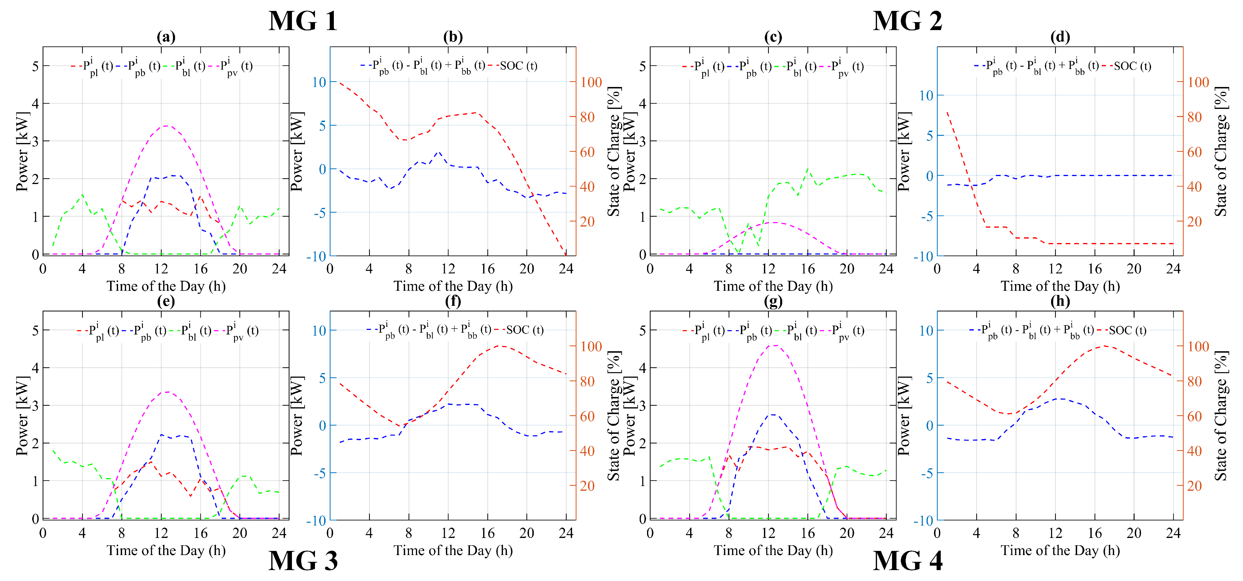
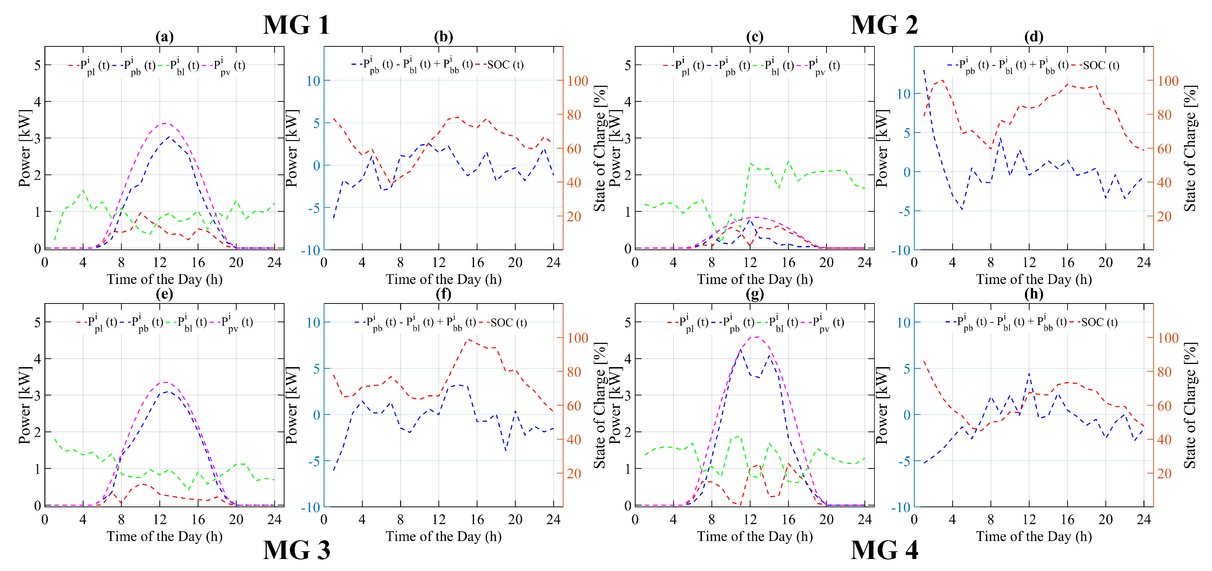
6. Simulation Results and Discussion

In this section, the simulation results of heuristic state flow and the proposed optimization based energy management strategy are discussed for each case separately.

Case A: In case A, as the $SO{C}_{initial}$ of ESSs for the 2nd and 3rd MGs is assumed at 20% of $B_{max}$, while the $SO{C}_{initial}$ of ESSs for remaining two MGs is at 100% of $B_{max}$, therefore, it is obvious that there will be some power deficiency at the 2nd and 3rd MGs, because the available power from each ESS is not enough to run the load during the off-sunlight hour. Furthermore, as soon as the SOC of ESS will reach its $B_{min}$, then there will be no power source available to charge it. In the heuristic state flow based strategy, as seen in Figure 6d, for the 2nd MG the SOC of ESS during time interval $t=0$ to $t=4$ keeps decreasing until it reaches to zero at $t=4$. Similarly, as seen in Figure 6f, for the 3rd MG, the SOC of ESS from $t=0$ to $t=4$ h keeps decreasing to zero at $t=4$. During the time interval $t=4$ to $t=8$, the load of both MGs is run by neighboring MGs 1 and 4. Also, the SOC of ESS for both MGs remains at zero during this time interval, showing that both surplus neighboring MGs supplied the exact amount of power required to run the load during this time interval. As soon as the PV panel starts generating power, the SOC of ESS of each MG starts increasing until $t=16$ as seen in Figure 6b,d,f,h. The ESS of each MG keeps on charging as long as power generated by the PV panel is greater than the load during time interval $t=8$ to $t=16$ (see Figure 6a,c,e,g). From $t=16$ to $t=24$, the SOC of ESS of each MG again starts decreasing because the power generated by PV panel is either zero or less than the load. Therefore, the excess load is now being run by the available charge of the ESS for the remaining time cycle.

Figure 6. Power flow of various system variables of each microgrid using heuristic state flow based energy management strategy for case A. (a,c,e,g) Power flow of PV, battery and Load, (b,d,f,h) Battery charging/discharging and state of charge.

On other hand, for the optimization based strategy, as seen in Figure 7d, for the 2nd MG during time interval $t=0$ to $t=4$, using a day ahead forecasted data of PV generation and load profile of the ESS, starts receiving power from neighboring MGs irrespective of the available SOC, load, and PV generation. Similarly, as seen in Figure 7f, for the 3rd MG during the time interval $t=0$ to $t=4$, the SOC of ESS starts increasing as the power flow for this interval is positive, showing that ESS is in charging mode. The power flow of the ESSs of the 1st and 4th MG is negative, which shows that both ESSs are in discharging mode, as seen in Figure 7b,h. Besides supplying power to their own loads, both surplus MGs are also supplying some amount of power to their neighboring MGs with power shortages. During the time interval $t=4$ to $t=8$, the load of both deficient MGs is run by their own ESS, as both have enough SOC to run their load, which is not the case in the heuristic strategy. As soon as the PV panel starts generating power, the SOC of the ESS of each MG starts increasing until $t=16$ as seen in Figure 7b,d,f,h. From $t=16$ to $t=24$, the SOC of ESS of each MG again starts decreasing, since the power generated by the PV panel is either zero or less than the load provided at that time. Therefore, the excess load is now run by the available ESS charge for the remaining time cycle. The main advantage of the proposed strategy here is the basis of decision making on the forecasted data of PV generation and MG load for a 24-h cycle, not the instant value of load, SOC of ESS, and PV generation. This decision making basis ensures the SOC of MG ESS remains balanced and above the minimum value.

Figure 7. Power flow of various system variable of each microgrid using proposed optimization based energy management strategy for case A. (a,c,e,g) Power flow of PV, battery and Load, (b,d,f,h) Battery charging/discharging and state of charge.

Case B: In case B, the 2nd load is doubled as compared to its normal day load; however, the installed PV system size and generation is the same as the normal day load. The load, PV generation, and SOC of ESS of all remaining MGs is the same as of the normal day. It is obvious that there will be some power shortage at the 2nd, because the available power from ESS and PV generation is not enough to run the load for complete daily cycle. Further, as soon as ESS reached $B_{min}$, there would be no power available to charge it. For the heuristic state flow based strategy, as seen in Figure 8d, for the 2nd MG the SOC of ESS during time interval $t=0$ to $t=8$ keeps decreasing, as there is no PV power available to charge ESS. The negative value of power flow shows that it keeps discharging during this time interval. Similarly, as seen in Figure 8b,f,h, the SOC of all other remaining MGs also keeps decreasing for said time interval, but the discharging rate is not as fast as for the 2nd MG. As soon as the PV panel starts generating power, the SOC of ESS of each MG starts increasing until $t=16$ as as seen in Figure 8b,d,f,h. As also seen from Figure 8d, the ESS of the 2nd MG is in charging mode during $t=8$ to $t=12$, as power flow is positive. The ESS of each MG keeps charging as long as the power generated by the PV panel is more than the load, as shown in Figure 8a,c,e,g. During time interval $t=16$ to $t=24$, the SOC of ESS of each MG again starts decreasing, because the power generated by the PV panel is either zero or less than the load at that time. Therefore, the excess load is now run by the available charge of ESS for the remaining time cycle. At the end of the cycle the SOC of ESS of each MG is at its default value, as the overall load is the same as the power generated by the PV system for 24 h. This is not the case for the 2nd MG, since the load is twice that of to the power generated by PV system. Therefore, the remaining load is run by ESS, which in turn decreases the SOC to zero for the next time cycle.

Figure 8. Power flow of various system variable of each microgrid using heuristic state flow based energy management strategy for case B. (a,c,e,g) Power flow of PV, battery and Load, (b,d,f,h) Battery charging/discharging and state of charge.

For the optimization based strategy, as seen in Figure 9d for 2nd MG, the SOC of ESS during the time interval $t=0$ to $t=8$ keeps decreasing until it reaches $B_{min}$. As soon as the PV system starts generating power during the time interval $t=8$ to $t=16$, the ESS of the 2nd MG remains in charging mode and charges the ESS to a sufficient level so that the load can be run easily during non-sunlight hours without violating the minimum threshold limit for the SOC. All other MGs continue switching between charging and discharging mode, depending on the available generated power and load as seen in Figure 9b,f,h. Similarly, as noticed in Figure 9a,c,e,f, the load is either run directly from the ESS during non-sunlight hours ($t=0$ to $t=8$ and $t=16$ to $t=24$) or by both ESS and PV power during sunlight hours ($t=8$ to $t=16$). Again, the main advantage of our proposed optimization based strategy is that it is not making a decision based on the instant values of load, SOC of ESS, and PV generation, but based on the forecasted data of PV generation and load of each MG for the complete daily time cycle. This strategy also ensures the available SOC of ESS in each MG (above the $B_{min}$) for next daily cycle.

Figure 9. Power flow of various system variables of each microgrid using proposed optimization-based energy management strategy for case B. (a,c,e,g) Power flow of PV, battery and Load, (b,d,f,h) Battery charging/discharging and state of charge.

Case C: In case C, the $SO{C}_{initial}$ of ESS for each MG is at 100% of its maximum value. The load of each MG is also same as the normal day load; however, PV generation of the 2nd and 4th MGs is at 10% of its normal day generation. Therefore, there will be some power shortage at the 2nd and 4th MGs since the generated power from the PV system is not enough to run the load in sunlight hours and also not enough to charge ESS for off sunlight hours. Further, as soon as ESS will go below $B_{min}$, there would be no power source available to recharge to or above its minimum value.

For the heuristic state flow based strategy, as seen in Figure 10d, for the 2nd MG, the SOC of ESS from $t=0$ to $t=24$ keeps decreasing to zero at $t=24$. Similarly, as seen in Figure 10h for the 4th MG, the SOC of ESS from $t=0$ to $t=24$ h also keeps decreasing to zero at $t=24$. As seen in Figure 10c,g, as soon as the PV system starts generating power in sunlight hours during the time interval $t=8$ to $t=16$, there is a slight change in the ESS discharging rate due to the need for a little power to run the load provided by PV system. Both the 1st and 2nd MGs keep working as normal throughout the day. During the time interval $t=0$ to $t=8$, the load of both MG is run by ESS. As soon as the PV panel starts generating power, the SOC of the ESS of each MG starts increasing until it reaches $t=16$ (see Figure 10a,e). The ESS of each MG keeps on charging as long as the power generated by the PV panel is more than the current load, as shown in Figure 10a,c,e,g. During the time interval $t=16$ to $t=24$, the SOC of ESS of each MG again starts decreasing, because the power generated by the PV panel is either zero or less than the load at that time. Therefore, the excess load is now run by the available charge of the ESS for the remaining time cycle.

Figure 10. Power flow of various system variable of each microgrid using heuristic state flow based energy management strategy for case C. (a,c,e,g) Power flow of PV, battery and Load, (b,d,f,h) Battery charging/discharging and state of charge.

For the optimization based strategy, as seen in Figure 11d,h for the 2nd and 4th MG, the SOC of the ESS during time interval $t=0$ to $t=8$ is decreasing. However, as soon as the PV systems of neighboring MGs start generating power, they also start supplying power to the deficient MGs (2nd and 4th) which in turn hold the SOC of ESS above the $B_{min}$. Both, the 1st and 2nd MGs continue as normal. During the time interval $t=0$ to $t=8$, the load of both MG is run by the ESS. As soon as the PV panel starts generating power, the SOC of the ESS of each MG starts increasing until it reaches $t=16$ (see Figure 11a,e). In our proposed optimization-based strategy, although the SOC of the 1st and 3rd MGs at $t=24$ is at 60% of its maximum value, less than the one in the heuristic-based strategy, the SOC of the 2nd and 4th MGs at $t=24$ is also at 50–60% of its maximum value, which is not the case in the heuristic-based strategy, as seen in Figure 11b,d,f,h. The main advantage of the proposed strategy in making decisions based on the forecasted data of PV generation and the load of each MG for a complete daily time cycle is evident in Figure 11a,c,e,g.

Figure 11. Power flow of various system variables of each microgrid using proposed optimization based energy management strategy for case C. (a,c,e,g) Power flow of PV, battery and Load, (b,d,f,h) Battery charging/discharging and state of charge.

Case D: In case D, the PV panel output of the 2nd MG is at 20% of its rated output, while the PV panel output of all three remaining MGs is at 100% of their rated output. The $SO{C}_{initial}$ of the ESS for the 2nd MG is at 20% of its $B_{max}$, while the $SO{C}_{initial}$ of the ESS for the remaining three MGs is at 100% of its $B_{max}$. The load of the 2nd MG is at 120% as compared to the normal day load, while the load of all remaining three MGs is at their normal load. Therefore, there will be some power shortage at the 2nd MG for similar reasons in previous cases. If the ESS goes below its minimum value or reaches zero, then there is no power source to recharge to above its minimum value. For the heuristic state flow based strategy, as seen in Figure 12d, for the 2nd MG the SOC of ESS during time interval $t=0$ to $t=4$ keeps decreasing until reaches zero at $t=4$. During the time interval $t=4$ to $t=24$, the load of the 2nd MG is run by the neighboring MG. As noticed, the SOC of the ESS of the 2nd MG is at a zero level until $t=24$. The MG with a power shortage receives only the same power level as the load from neighboring MGs. This proves that the heuristic state flow based strategy makes decisions on the current situation irrespective of previous and future load and generation, while all other MGs continue as normal with their daily load and generation. During the time interval $t=0$ to $t=8$, the load of both MGs is run by ESS. As soon as the PV panel starts generating power, the SOC of the ESS of each MG starts increasing until $t=16$ as seen in Figure 12a,e. The ESS of each MG keeps charging as long as the power generated by the PV panel is more than the current load, as shown in Figure 12a,c,e,g. From $t=16$ to $t=24$, the SOC of the ESS of each MG again starts decreasing due to the power generated by the PV panel being either zero or less than the load at that time. Therefore, the excess load is now being run by the available SOC of ESS for the remaining time cycle.

Figure 12. Power flow of various system variable of each microgrid using heuristic state flow based energy management strategy for case D. (a,c,e,g) Power flow of PV, battery and Load, (b,d,f,h) Battery charging/discharging and state of charge.

For the proposed strategy, as seen in Figure 13d, for the 2nd MG, the ESS starts charging from its neighboring MGs at $t=0$. Then, from $t=0$ to $t=24$, all MGs continue switching between charging and discharging mode depending on forecasted load and generation data of their own system as well as their neighboring MGs, as seen in Figure 13a,c,e,g. Further, in our proposed optimization-based strategy, although the SOC of the 3rd and 4th MG at $t=24$ is at 40–60% of its maximum value, which is less than the one belonging to the heuristic-based strategy, the SOC of the 1st and 2nd MG at $t=24$ is also at 50–60% of its maximum value, which is not the case in the heuristic-based strategy, as seen in Figure 13b,d,f,h. The main advantage of our proposed optimization-based strategy can be seen from Figure 13a,c,e,g, as the previous cases where the EMS ensures that the SOC of the ESS of each MG always remains above the minimum value for next daily cycle. The SOC of each MG ESS at the end of the time cycle $t=T$ for all case studies discussed above is shown in Table 3. In the heuristic state flow-based model, for case A, the SOC of the ESS of the 2nd MG at t = T (end of time cycle) is at 39% of its maximum value. Similarly, for case B, the SOC of the ESS of the 2nd MG at t = T is at 0% of its maximum value. For case C, the SOC of the ESS of the 2nd and 4th MGs at t = T is at 5% of its maximum value. For case D, the SOC of ESS of 1st and 2nd MGs at t = T is at 5% and 0% of its maximum value, respectively. In our proposed optimization based model, in all cases (A–D), the SOC of the ESS of all MGs is always above the minimum allowed SOC of the ESS. The computational cost of solving the proposed problem for all case studies is shown in Table 4. This information shows that our proposed optimization-based model is applicable in actual decision making in the day-ahead market. As the problem solving time taken in each case study is less than 10 min, the same proposed model is also applicable even for 15–30 min ahead decision making depending on the data availability.

Figure 13. Power flow of various system variable of each microgrid using proposed optimization based energy management strategy for case D. (a,c,e,g) Power flow of PV, battery and Load, (b,d,f,h) Battery charging/discharging and state of charge.

Table 3. State of charge (SOC) (%) of each microgrid at end of time cycle (t = T).

Case	Heuristic State Flow Based Model				Proposed Optimization Based Model
	1	2	3	4	1	2	3	4
A	60	39	65	60	75	65	60	58
B	80	0	80	80	80	60	60	65
C	80	05	80	05	60	40	55	45
D	05	0	80	80	60	60	58	45

Table 4. Computational cost of solving proposed problem using MATLAB 2020.

Case	Computational Cost
	Heuristic State Flow	Proposed
A	0.182 s	390.18 s
B	0.175 s	355.10 s
C	0.266 s	246.12 s
D	0.112 s	432.14 s

7. Conclusions

In this work, we propose a simultaneous, two-stage, day-ahead energy management strategy for MMGs and individual MG distribution system with several DGs, ESSs, and consumption units. The proposed optimization strategy for EMS simultaneously controls the energy scheduling, minimizes the main grid dependency, and enhances the flexibility of the MMG system by maximizing the stored energy in the ESSs and discharging the EMS when required.

In the heuristic state flow-based EMS, the EMS only considers load demand and solar irradiance at the current time instant, irrespective of previous and forecasted values. In our proposed two-stage optimization strategy, the EMS simultaneously incorporates previous and foretasted values of all DGs, ESSs, and consumption units connected in the MMG distribution network, and the total grid dependency reduces to zero, and depth of discharge (DoD) of ESSs increases up to 50%. Future work includes evaluation of proposed day ahead energy management for multi microgrids in hardware-in-loop (HIL) by mitigating the complexity of the system control and by optimizing the power-sharing requirements.

References

1. Chen, S.; Liu, P.; Li, Z. Low carbon transition pathway of power sector with high penetration of renewable energy. Renew. Sustain. Energy Rev. 2020, 130, 109985. [Google Scholar] [CrossRef]
2. Global, E. Outlook 2019: Scaling Up the Transition to Electric Mobility, May 2019; International Energy Agency: Paris, France, 2019.
3. Chaouachi, A.; Kamel, R.M.; Andoulsi, R.; Nagasaka, K. Multiobjective intelligent energy management for a microgrid. IEEE Trans. Ind. Electron. 2012, 60, 1688–1699. [Google Scholar] [CrossRef]
4. Mansour-Saatloo, A.; Agabalaye-Rahvar, M.; Mirzaei, M.A.; Mohammadi-Ivatloo, B.; Abapour, M.; Zare, K. Robust scheduling of hydrogen based smart micro energy hub with integrated demand response. J. Clean. Prod. 2020, 267, 122041. [Google Scholar] [CrossRef]
5. Suberu, M.Y.; Mustafa, M.W.; Bashir, N. Energy storage systems for renewable energy power sector integration and mitigation of intermittency. Renew. Sustain. Energy Rev. 2014, 35, 499–514. [Google Scholar] [CrossRef]
6. Alizadeh Bidgoli, M.; Payravi, A.R.; Ahmadian, A.; Yang, W. Optimal day-ahead scheduling of autonomous operation for the hybrid micro-grid including PV, WT, diesel generator, and pump as turbine system. J. Ambient. Intell. Humaniz. Comput. 2021, 12, 961–977. [Google Scholar] [CrossRef]
7. Zia, M.F.; Elbouchikhi, E.; Benbouzid, M. Microgrids energy management systems: A critical review on methods, solutions, and prospects. Appl. Energy 2018, 222, 1033–1055. [Google Scholar] [CrossRef]
8. Hussain, A.; Bui, V.H.; Kim, H.M. Microgrids as a resilience resource and strategies used by microgrids for enhancing resilience. Appl. Energy 2019, 240, 56–72. [Google Scholar] [CrossRef]
9. Karimi, H.; Jadid, S.; Makui, A. Stochastic energy scheduling of multi-microgrid systems considering independence performance index and energy storage systems. J. Energy Storage 2021, 33, 102083. [Google Scholar] [CrossRef]
10. Arefifar, S.A.; Mohamed, Y.A.R.I.; El-Fouly, T. Optimized multiple microgrid-based clustering of active distribution systems considering communication and control requirements. IEEE Trans. Ind. Electron. 2014, 62, 711–723. [Google Scholar] [CrossRef]
11. Ilic, M.D. From hierarchical to open access electric power systems. Proc. IEEE 2007, 95, 1060–1084. [Google Scholar] [CrossRef] [Green Version]
12. Shoeb, M.A.; Shafiullah, G.; Shahnia, F. Coupling Adjacent Microgrids and Cluster Formation under a Look-Ahead Approach Reassuring Optimal Operation and Satisfactory Voltage and Frequency. IEEE Access 2021, 9, 78083–78097. [Google Scholar] [CrossRef]
13. Backhaus, S.N.; Dobriansky, L.; Glover, S.; Liu, C.C.; Looney, P.; Mashayekh, S.; Pratt, A.; Schneider, K.; Stadler, M.; Starke, M.; et al. Networked Microgrids Scoping Study; Technical Report; Los Alamos National Lab. (LANL): Los Alamos, NM, USA, 2016.
14. Hussain, A.; Bui, V.H.; Kim, H.M. A resilient and privacy-preserving energy management strategy for networked microgrids. IEEE Trans. Smart Grid 2016, 9, 2127–2139. [Google Scholar] [CrossRef]
15. Datta, U.; Kalam, A.; Shi, J. Electric Vehicle (EV) in Home Energy Management to Reduce Daily Electricity Costs of Residential Customer; NISCAIR-CSIR: New Delhi, India, 2018. [Google Scholar]
16. Chowdhury, N.; Hossain, C.A.; Longo, M.; Yaïci, W. Optimization of solar energy system for the electric vehicle at university campus in Dhaka, Bangladesh. Energies 2018, 11, 2433. [Google Scholar] [CrossRef] [Green Version]
17. Khalid, M.; Ahmadi, A.; Savkin, A.V.; Agelidis, V.G. Minimizing the energy cost for microgrids integrated with renewable energy resources and conventional generation using controlled battery energy storage. Renew. Energy 2016, 97, 646–655. [Google Scholar] [CrossRef]
18. Hossain, C.A.; Chowdhury, N.; Longo, M.; Yaïci, W. System and cost analysis of stand-alone solar home system applied to a developing country. Sustainability 2019, 11, 1403. [Google Scholar] [CrossRef] [Green Version]
19. Nasir, M.; Iqbal, S.; Khan, H.A. Optimal planning and design of low-voltage low-power solar DC microgrids. IEEE Trans. Power Syst. 2017, 33, 2919–2928. [Google Scholar] [CrossRef]
20. Van der Meer, D.; Mouli, G.R.C.; Mouli, G.M.E.; Elizondo, L.R.; Bauer, P. Energy management system with PV power forecast to optimally charge EVs at the workplace. IEEE Trans. Ind. Inform. 2016, 14, 311–320. [Google Scholar] [CrossRef] [Green Version]
21. Moayedi, S.; Davoudi, A. Unifying distributed dynamic optimization and control of islanded DC microgrids. IEEE Trans. Power Electron. 2016, 32, 2329–2346. [Google Scholar] [CrossRef]
22. Xiao, J.; Wang, P.; Setyawan, L. Multilevel energy management system for hybridization of energy storages in DC microgrids. IEEE Trans. Smart Grid 2015, 7, 847–856. [Google Scholar] [CrossRef]
23. Loukarakis, E.; Bialek, J.W.; Dent, C.J. Investigation of maximum possible OPF problem decomposition degree for decentralized energy markets. IEEE Trans. Power Syst. 2014, 30, 2566–2578. [Google Scholar] [CrossRef] [Green Version]
24. Zhang, H.; Zhou, S.; Gu, W.; Zhu, C. Optimized operation of micro-energy grids considering the shared energy storage systems and balanced profit allocation. CSEE J. Power Energy Syst. 2022, 1–17. [Google Scholar] [CrossRef]
25. Tushar, M.H.K.; Zeineddine, A.W.; Assi, C. Demand-side management by regulating charging and discharging of the EV, ESS, and utilizing renewable energy. IEEE Trans. Ind. Inform. 2017, 14, 117–126. [Google Scholar] [CrossRef]
26. Xiao, D.; AlAshery, M.K.; Qiao, W. Optimal price-maker trading strategy of wind power producer using virtual bidding. J. Mod. Power Syst. Clean Energy 2021, 10, 766–778. [Google Scholar] [CrossRef]
27. Rana, R.; Prakash, S.; Mishra, S. Energy management of electric vehicle integrated home in a time-of-day regime. IEEE Trans. Transp. Electrif. 2018, 4, 804–816. [Google Scholar] [CrossRef]
28. Ali, Z.; Putrus, G.; Marzband, M.; Tookanlou, M.B.; Saleem, K.; Ray, P.K.; Subudhi, B. Heuristic Multi-Agent Control for Energy Management of Microgrids with Distributed Energy Sources. In Proceedings of the 2021 56th International Universities Power Engineering Conference (UPEC), Middlesbrough, UK, 31 August–3 September 2021; IEEE: Piscataway, NJ, USA, 2021; pp. 1–6. [Google Scholar]
29. Abdalla, M.A.A.; Min, W.; Mohammed, O.A.A. Two-stage energy management strategy of EV and PV integrated smart home to minimize electricity cost and flatten power load profile. Energies 2020, 13, 6387. [Google Scholar] [CrossRef]
30. Mao, M.; Jin, P.; Hatziargyriou, N.D.; Chang, L. Multiagent-based hybrid energy management system for microgrids. IEEE Trans. Sustain. Energy 2014, 5, 938–946. [Google Scholar] [CrossRef]
31. Xiao, J.; Wang, P.; Setyawan, L.; Xu, Q. Multi-level energy management system for real-time scheduling of DC microgrids with multiple slack terminals. IEEE Trans. Energy Convers. 2015, 31, 392–400. [Google Scholar] [CrossRef]
32. Pervaiz, S.; Khan, H.A. Low irradiance loss quantification in c-Si panels for photovoltaic systems. J. Renew. Sustain. Energy 2015, 7, 013129. [Google Scholar] [CrossRef]
33. Forniés, E.; Naranjo, F.; Mazo, M.; Ruiz, F. The influence of mismatch of solar cells on relative power loss of photovoltaic modules. Sol. Energy 2013, 97, 39–47. [Google Scholar] [CrossRef]
34. Solanki, C.S. Solar Photovoltaics: Fundamentals, Technologies and Applications; Phi Learning Pvt., Ltd.: New Delhi, India, 2015. [Google Scholar]
35. Sengupta, M.; Xie, Y.; Lopez, A.; Habte, A.; Maclaurin, G.; Shelby, J. The national solar radiation data base (NSRDB). Renew. Sustain. Energy Rev. 2018, 89, 51–60. [Google Scholar] [CrossRef]
36. Nadeem, A.; Arshad, N. PRECON: Pakistan Residential Electricity Consumption Dataset. In Proceedings of the Tenth ACM International Conference on Future Energy Systems (e-Energy ’19), Phoenix, AZ, USA, 25–28 June 2019; ACM: New York, NY, USA, 2019; pp. 52–57. [Google Scholar] [CrossRef]