Machine Learning for Solar Resource Assessment Using Satellite Images

Abstract

Understanding solar energy has become crucial for the development of modern societies. For this reason, significant effort has been placed on building models of solar resource assessment. Here, we analyzed satellite imagery and solar radiation data of three years (2012, 2013, and 2014) to build seven predictive models of the solar energy obtained at different altitudes above sea level. The performance of four machine learning algorithms was evaluated using four evaluation metrics, MBE, R², RMSE, and MAPE. Random Forest showed the best performance in the model with data obtained at altitudes below 800 m.a.s.l. The results achieved by the algorithm were: 4.89, 0.82, 107.25, and 41.08%, respectively. In general, the differences in the results of the machine learning algorithms in the different models were not very significant; however, the results provide evidence showing that the estimation of solar radiation from satellite images anywhere on the planet is feasible.

1. Introduction

Nowadays, many countries depend on electrical energy generated by large-scale hydroelectric plants and fossil fuels, whereas the percentage of energy obtained from renewable sources remains low [1,2]. For this reason, great efforts have been made to obtain clean energy from removable sources such as the sun and the wind [3].

However, the viability of the use of these types of energy in a specific location depends on their availability (sun, wind, etc.) in the specific geographical location and on the energy requirements. Traditionally, data from monitoring stations have been used to determine this potential; however, the number of stations and sensors is limited. For this reason, the research community has been working on building mathematical, statistical, and predictive models for solar resource assessment [4].

The use of solar energy depends on the knowledge about the behavior of solar radiation in a specific geographical location; therefore, numerous studies have revolved around the feasibility of the solar resource based on data obtained from monitoring stations and meteorological satellites. Ordoñez-Palacios et al. [5] aimed at predicting solar radiation resources in photovoltaic systems using diverse machine learning techniques. In regression, the multilayer perceptron algorithm showed the highest performance, according to R² and RMSE, with values of 0.9 and 77.37, respectively. In classification, the AdaBoost ensemble method achieved the best results according to the accuracy, precision, recall, and F1-score metrics, with values of 0.94, 0.90, 0.99, and 0.94, respectively.

Nwokolo et al. [6] estimated the global solar radiation potential using improved probabilistic Ångstrom–Prescott and Gumbel models. In total, 29 Ångstrom–Prescott (AP) empirical models were analyzed, revealing the parameters of each model, its parental season, and the bibliographic source. The M1–M3 models were fitted using generalized data sets. The M4–M20 models were acquired from the literature. The M21–M29 models were fitted using the data sets obtained from measurement stations in Nigeria. The M13 model obtained the lowest values of RMSE = 0.0001 and RRMSE = 0.0176% and the corresponding maximum value of R² = 0.990 and GPI = 0.9321.

Similarly, Geetha et al. [7] made predictions of hourly solar radiation using different Artificial Neural Network (ANN) models. The best ANN model showed an R² of 0.9376 for the training data and 0.9340 for the test data. The findings revealed that the ANN model may be used to effectively estimate the hourly average solar radiation, even in the absence of monitoring facilities.

On the other hand, Oyewola et al. [8] showed that the inclusion of air temperature and humidity as the two main predictors, along with duration of sunlight, day length, and extraterrestrial radiation, improves the global solar radiation predictions. The authors adopted 20 empirical models based on their simplicity and the availability of the predictive parameters over 35 years (1984–2018) from six weather stations in the Fiji Islands. The models with the most reliable values of global solar radiation showed an R² between 0.415 and 0.988 at a confidence level of 95%.

Alrashidi et al. [9] introduced a framework that integrates Support Vector Regression, the grasshopper optimization algorithm, and the feature selection algorithm to forecast global solar radiation. The performance of the proposed predictive model (SVR-GOA-BA), applied to the locations of Dhahran, Riyadh, and Jeddah, in Saudi Arabia, obtained an R² of 0.98823481, 0.98863249, and 0.98883136 and an RMSE of 45.0903, 49.8129, and 41.1592 for each site, respectively.

Finally, Ağbulut et al. [10] evaluated the performance of different machine learning algorithms for the daily prediction of global solar radiation. The results show that the R², MABE, and RMSE values of all algorithms ranged from 0.855 to 0.936, from 1.870 to 2.328 MJ/m², and from 2.273 to 2.820 MJ/m², respectively. k-NN exhibited the worst results for all the metrics.

Other studies focused on the prediction of solar radiation using images. Ajith and Martínez-Ramón [11] aimed at forecasting solar radiation using deep learning and the fusion of infrared cloud imagery and radiation data. The work used the metrics MAPE, R², RMSE, MAE, and the t-statistic for the proposed networks and other reference models for cloudy days. The proposed CNN-L and MICNN-L models outperformed time series-based methodologies with a minimum MAPE of 2.00 and 2.96, respectively. Similarly, the MAE was reduced by 43.75% (from 0.016 to 0.009) for CNN-L and by 31.25% (from 0.016 to 0.011) for MICNN-L compared with the reference model with the best performance.

Rodríguez-Benitez et al. [12] evaluated new solar radiation forecasting methods based on satellite imagery and sky cameras. The study, carried out at a site in southern Spain, revealed that the use of models based on all-sky imagery (ASI), which consists of a set of three video surveillance cameras, provides little benefit compared with the use of satellite-based models for the nowcasting of solar radiation.

Magnone et al. [13] used cloud motion identification algorithms based on full-sky images to support solar radiation forecasting. Three different cloud motion algorithms were considered, heuristic motion detection (HMD), particle image velocimetry (PIV), and a persistent model. The results show that the integration of the forecast cloud cover information in the circumsolar area leads to a decrease in the width of forecast global horizontal irradiance (GHI) intervals by up to 2% for forecast horizons in the range of 1–10 min.

Similarly, the study by Si et al. [14] proposed a new hybrid method to forecast global horizontal radiation combining satellite images and meteorological information. It could be seen that the use of three continuous satellite images contributes to the improvement of the forecast accuracy of global horizontal irradiance several hours in advance, leading to excellent performance produced by the hybrid approach of combining meteorological data and factors of cloud cover, extracted from satellite images.

Li [15] made short-term PV energy predictions based on clear-sky data from a moderate-resolution imaging spectroradiometer. Polycrystalline silicon photovoltaic panels of 1.2 kW of the same specifications were selected, divided into five groups, and placed at different tilt angles. A representative clean panel of 35° tilt was taken as the verification object, with data obtained prior to 16 December 2018, and trained to predict PV power from 9:00 a.m. to 15:00 p.m. daily from 17 December 2018. The accuracy of the experimental process was demonstrated by practical engineering verification.

Alonso-Suárez [16] built a model based on satellite imagery that allows one to build monthly and annual maps of solar potential. The model represents the second version of the Solar Map of Uruguay (MSUv2) and constitutes an advance in the quantity and quality of the information available on the long-term behavior of the resource. This new version increases the accuracy of the annual and monthly mapping from 2% to 15% and increases the spatial resolution from 150 km to 3 km. In addition, it includes components of solar radiation that had not been considered to date and a map of photovoltaic generation potential.

Yang et al. [17] analyzed the main aspects related to the evaluation and forecast of the solar resource. Solar resource assessment focuses primarily on ground-based measurement data, remote-sensing retrieved data, and output of numerical weather prediction models. Solar forecasting has five main aspects: forecasting methodology, post-processing, irradiance-to-power conversion, verification, and materialization of values. In this sense, this work proposes a predictive model of solar radiation as part of an evaluation process of solar resources.

Solar radiation estimation models can be mathematical, statistical, and predictive. In that sense, it is important to highlight that the data sets used in this research study were obtained from satellite images using a mathematical model. Subsequently, these data and the observed solar radiation were integrated to form a data set for each geographic location. In that order of ideas, our model is hybrid, because it uses a mathematical model to obtain data from satellite images and a predictive machine learning model to look for patterns in the data that lead to the prediction of solar radiation. In the present research study, images of 1447 × 1636 pixels from the years 2012, 2013, and 2014 from the GOES-13 meteorological satellite [18] were processed. With these data, (i) the features in the data sets were obtained through a mathematical model; (ii) three models (M1–M3) were built to estimate solar radiation, using data extracted from the images at geographical points located at different altitudes; (iii) three models (M5–M7) were built with a sample of 6500 records from each geographic location; (iv) a model (M4) was built with data from all geographic locations. The models used the following variables: reflectance, cloudiness index, bright sunshine hours, solar radiation at the edge of the atmosphere, and solar radiation observed by the monitoring station. The study seeks to determine if altitude affects the prediction of solar radiation.

The rest of the document includes the following sections: Materials and Methods, Results, Discussion, and, finally, Conclusions.

2. Materials and Methods

This section exposes the questions of interest that guided the research project, the information sources for building the models, the way in which data were processed, and the tools used to build solar radiation prediction models.

2.1. Questions of Interest

Renewable energy sources can be transformed into electrical energy through systems designed for their use, and it is essential to know their availability in a specific geographical location, using measuring instruments, or mathematical, statistical, or predictive models. The photovoltaic industry constitutes a viable option to satisfy the growing demand for energy and the imperative need to reduce the carbon footprint, according to the works of Abdoli et al. [19] and Carneiro et al. [20].

The number of monitoring stations for environmental variables is limited. Due to this, it is necessary to build models for the prediction of solar radiation. These models can be obtained using variables from satellite imagery; therefore, it is crucial to answer the following questions: What is the process to extract variables from satellite images? Which machine learning techniques have the best performance in the prediction of solar radiation? What is the performance of the models if a sample of the total data is used? Which metrics are used to evaluate the results of the models? Does the altitude of a geographical location affect the results of the predictions? These questions are answered in the different sections of this paper.

2.2. Sources of Information

Table 1. Satellite imagery.

ID	Year	Number of Images	Approximate Size	Size after Processing
1	2012	1991 out of 4758	1991 out of 4758	1991 out of 4758
2	2013	9–20 MB	9–20 MB	9–20 MB
3	2014	2.3 MB	2.3 MB	2.3 MB

,

Table 2. Data sets from the DAGMA stations.

ID	Station	Latitude	Longitude	Altitude (m.a.s.l)	Years	Hourly Records
1	ERA	3.44779	−76.51918	968	2012–2014	18,705
2	Compartir	3.42823125782003	−76.46654484665319	952	2014	6270
3	Univalle	3.3780	−76.53388889	996	2012–2014	12,337

and

Table 3. Data set from the IDEAM stations.

ID	Station	Latitude	Longitude	Altitude (m.a.s.l)	Years	Hourly Records
1	Acueducto Mocoa (Putumayo)	1.157333333	−76.65183333	650	2012–2014	17,480
2	El Pepino (Putumayo)	1.082888889	−76.66711111	760	2012–2014	9029
3	Florencia (Caquetá)	1.7330	−75.64502778	600	2012–2014	8306
4	Macagual (Caquetá)	1.50	−75.66	280	2012, 2014	5045
5	Botana-Pasto (Nariño)	1.16	−77.27880556	2820	2012–2014	21,828
6	Estrecho Patía (Cauca)	1.96	−77.12	720	2012–2014	12,088
7	Aeropuerto Guapi (Cauca)	2.574416667	−77.89475	42	2014	1397
8	Inzá (Cauca)	2.548194444	−76.06394444	1800	2012–2014	6724
9	La Sierra (Cauca)	2.193833333	−76.75033333	1870	2012, 2014	2071

depict the images and data sets used. The historical images were obtained from the visible spectral channel of the GOES-13 weather satellite. The dimensions of each image are 1447 × 1636 pixels and 16 bits per pixel. Likewise, solar radiation data sets were used from the Administrative Department of Environmental Management DAGMA (Cali Mayor’s Office, Colombia), and the Institute of Hydrology, Meteorology and Environmental Studies, IDEAM. Each pixel in the image represents a specific location with geographic coordinates represented by latitude and longitude values. The images were taken in ranges between 6 and 18 h; however, some days of the year do not have all the images.

The images were obtained from the website of the CLASS library of the National Oceanic and Atmospheric Administration (NOAA) [21]. These images were processed using NOAA Weather and Climate Tools (WCT) [22] to transform them into binary format files with an NC extension (which stores multidimensional data organized in matrices). Subsequently, python geographic information libraries (Rasterio and Pyproj) were used to convert these files into GeoTIFF files (a metadata standard that allows georeferenced information to be embedded in a TIFF image). GeoTIFF allows the digital level of coordinates to be extracted from the image so that reflectance and the cloud index can be calculated.

According to the work of the researcher Poveda Matallana [23], the digital level of the image ($nd$) and the satellite calibration coefficient ($k$) [24] enable the calculation of the nominal reflectance $\left(R_{prev}\right)$ (1) to be conducted; the monthly correction factor ($C$) of the satellite [25] and the nominal reflectance allow one to calculate the back reflectance ($R_{post}$) (2). Finally, the back reflectance enables the calculation of the pixel reflectance ($R_p$) (3) of each image; to this end, the calculation of the astronomical variable distance from the Earth to the Sun ($r$) and the zenith angle (${\theta }_z$) are also required.

$$R_{prev}=k \left(nd-29\right)$$

(1)

$$R_{post}=C\ast R_{prev}$$

(2)

$$R_p=\left(R_{post}\ast r^2\right) cos\left({\theta }_z\right)$$

(3)

With the data obtained, the cloudiness index can be calculated ($n_c$) (4), from the maximum ($R_{max}$) and minimum ($R_{min}$) reflectance for every hour of the day. The exact value of the minimum reflectance and 80% of the maximum reflectance must be taken. In addition, the values of the cloudiness index must be between 0 and 1; therefore, they must be adjusted if they overflow outside the domain [26].

$$n_c=\left(R_p-R_{min}\right) \left(R_{max}-R_{min}\right)$$

(4)

The theoretical variables of daily sunshine hours ($N$) and daily extraterrestrial solar radiation ($H_{ext}$) are obtained from the calculation of other astronomical variables, such as solar declination, the equation of time, true solar time, and the astronomical length of the day.

The number of records of each solar radiation data set was reduced according to the number of images available. This is because the variables of each image were integrated with the measured solar radiation, thus forming the data sets to be used to build the predictive models.

Table 4. Data sets used for each model.

Model	Data Sets	Records
M1	Putumayo: Acueducto Mocoa, El Pepino; Cauca: Estrecho Patía, Aeropuerto Guapi; Caquetá: Florencia, Macagual	14,468
M2	Valle del cauca: ERA (Escuela República Argentina), Compartir, Univalle	8299
M3	Cauca: Inzá, La Sierra; Nariño: Botana (Pasto)	6856
M4	All the data sets	29,623

summarizes the number of records of the data sets used for each model.

The data sets were grouped considering the altitude of each monitoring station as follows: Model M1 included data from locations below 800 m.a.s.l. Model M2 used data from locations between 950 and 1000 m.a.s.l. Model M3 used data sets from locations above 1800 m.a.s.l. Model M4 integrates all data sets. Finally, considering that the first three models have significant differences in the number of records, an additional study was carried out with a random sample of 6500 records for each model (M5–M7), thus preventing the results from being affected by the number of records.

2.3. Machine Learning Algorithms

Regression models were implemented in python and Jupyter Notebooks. For data preparation, the RobustScaler method was used to normalize the data and prevent the results of the algorithms from being affected by outliers. The data were divided into training and test data (30% for test data). Four machine learning techniques were analyzed: Multiple Linear Regression, Support Vector Regression (SVR), Random Forest (RF), and Artificial Neural Network (ANN).

2.3.1. Multiple Linear Regression

This algorithm from Scikit Learn fits a linear model with coefficients w to minimize the residual sum of squares between the observed targets in the data set and the targets predicted by the linear approximation. Considering the simplicity of the method and the poor performance of the results, it was not necessary to adjust the hyperparameters.

2.3.2. Support Vector Regression (SVR)

The SVR algorithm is a variant of the support vector machine (SVM), which finds a hyperplane that maximizes the separation margin between classes. Different configurations were tested on the parameters for the kernel type that the algorithm uses, the tolerance for the stopping criteria, the degrees of the function for the polynomial kernel, the kernel coefficient for ‘rbf’, ‘poly’, and ‘sigmoid’, and the regularization parameter.

2.3.3. Random Forest (RF)

The Random Forest algorithm is an ensemble method that uses a set of decision trees to better generalize and avoid overfitting. We tuned the algorithm by varying the following hyperparameters: the number of trees, the number of features to consider in each split, the maximum number of levels in the tree, the minimum number of samples required to split a node, the minimum number of samples required at each leaf node, and the sample selection method to train each tree.

2.3.4. Artificial Neural Network (ANN)

The Multi-Layer Perceptron (MLP) is a supervised learning algorithm that learns by training on a data set. Given a set of features and a target, it can learn a non-linear function approximator for either classification or regression. Different configurations were tested with seven different hyperparameters, such as the optimization algorithm, the number of hidden layers, the L2 regularization term, the activation function, the learning rate, the maximum number of iterations, and the maximum number of epochs.

We used the randomized search method (RandomizedSearchCV) from the Scikit Learn library to tune the hyperparameters of each model. RandomizedSearchCV allows one to find hyperparameter values that achieve accuracy results similar to the hyperparameters returned by the grid search method (GridSearchCV) but significantly reduces the processing time. In contrast to GridSearchCV, RandomizedSearchCV simply performs sampling from the defined distribution. Furthermore, we used cross-validation (RepeatedKFold) to improve the accuracy performance of each model and to avoid overfitting. The implemented cross-validation randomly divided the data into 10 subsets and used RMSE as the loss function to optimize.

Seven regression models were built for the prediction of solar radiation: 3 models (M1–M3) using 100% of the data sets and 3 models (M5–M7) using a sample of 6500 records for locations with altitudes below 800 m.a.s.l, locations with altitudes between 950 and 1000 m.a.s.l, and locations with altitudes above 1800 m.a.s.l, respectively; additionally, 1 model (M4) was created using 100% of all data sets. Each model included variables obtained from satellite images (reflectance, cloudiness index), the sunlight hours, extraterrestrial solar radiation, and solar radiation. These variables were measured in diverse meteorological stations.

Table 5. Variables’ description.

ID	Variable	Description
1	Reflectance	It represents the value of solar radiation reflected by clouds.
2	Cloudiness index	It is a value related to cloud conditions: clear sky, partly cloudy, and cloudy (0-1).
3	Extraterrestrial solar radiation	It corresponds to the value of the electromagnetic radiation emitted by the sun, before entering the atmosphere; it is measured in W/m2.
4	Sunshine hours	It is the time in hours during which the sun provides an effective sunshine.
5	Solar radiation (target variable)	It is the flow of energy received from the sun in the form of electromagnetic waves; it is measured in W/m2.

describes each of the variables.

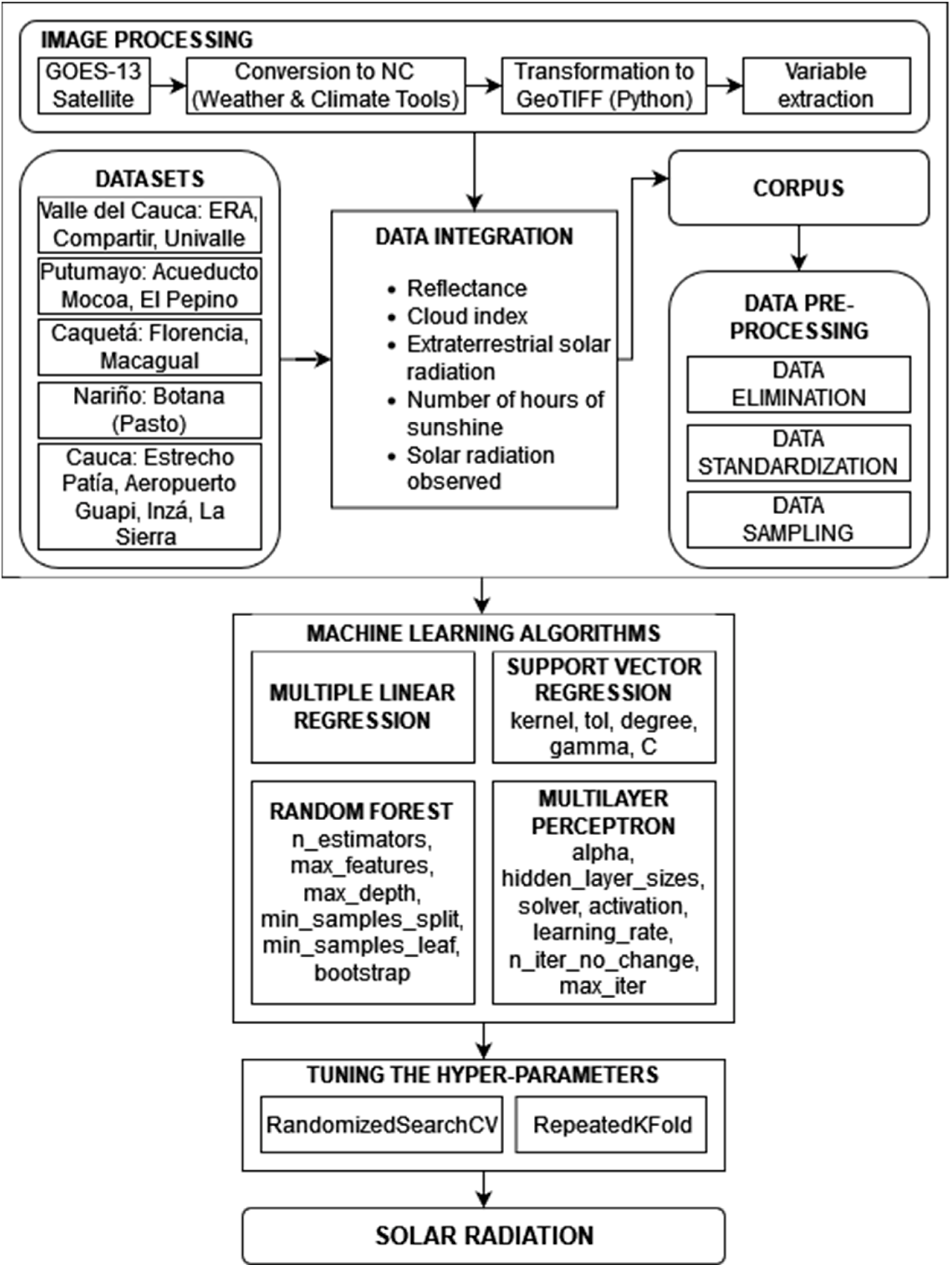
2.4. Model Architecture

Figure 1 depicts the data flow, from the information sources on the ground and on the satellite to the predictions of solar radiation using the regression algorithms, passing through the processing of the images, the integration, and the data processing.

2.5. Evaluation Metrics

The performance of the machine learning algorithms used in this work was evaluated using the following metrics: mean bias error (MBE), coefficient of determination (R²), root mean square error (RMSE) and the mean absolute percentage error (MAPE).

Table 6. Evaluation metrics.

Metric	Equation	Description	Performance Criteria
MBE	${\displaystyle \frac{1}{n}\sum _{i=1}^n}\left(y_i-x_i\right)$	Provides information on the long-term performance of the models. [27]	The closer it is to zero, the better the prediction result. [27]
R2	$1-{\displaystyle \frac{\sum {\left(y_i-x_i\right)}^2}{\sum {\left(x_i-\overline{x_i}\right)}^2}}$	Sets how well the actual data approximate the regression line. [27]	It ranges between 0 and 1; the closer it is to 1, the better the performance of the model. [27]
RMSE	$\sqrt{{\displaystyle \frac{1}{n}\sum _{i=1}^n}{\left(y_i-x_i\right)}^2}$	It represents the difference between actual and estimated values. [27]	It is a positive value, and the closer it is to zero, the better the estimation result. [27]
MAPE	${\displaystyle \frac{1}{n}\sum _{i=1}^n}\left|{\displaystyle \frac{x_i-y_i}{x_i}}\right|\times 100$	It explains how good a predictive model can be and measures the size of the errors as a percentage. [27]	As this value approaches zero, the performance of the model increases [27], considering the following categories [10]: High precision: MAPE ≤ 10%; Good: 10% < MAPE ≤ 20%; Reasonable: 20% < MAPE ≤ 50%; Low precision: MAPE > 50%.

exposes the equations, description, and performance criteria of each evaluation metric.

The data estimated by the models are represented by $y_i$, and the data obtained from the measurement stations are represented by $x_i$. Likewise, $\overline{x_i}$ represents the average of the measured data and $n$ the number of observations.

3. Results

According to R², RMSE and MAPE, Random Forest (RF) achieved the best performance (see

Table 7. Results obtained.

ID	Machine Learning Algorithms	Metrics	Locations with Altitudes below 800 m.a.s.l (M1, M5)		Locations with Altitudes between 950 and 1000 m.a.s.l (M2, M6)		Locations with Altitudes above 1800 m.a.s.l (M3, M7)		All the Data Sets (M4)
			100%	6500	100%	6500	100%	6500
1	Multiple Linear Regression	MBE	3.46	−1.26	1.85	−6.10	−2.02	−5.06	2.38
		R2	0.30	0.30	0.39	0.40	0.30	0.29	0.30
		RMSE	211.17	210.47	199.40	197.45	210.00	214.08	211.13
		MAPE	254.20	266.74	375.27	364.10	226.91	225.82	298.30
2	Support Vector Regression	MBE	1.81	2.75	0.60	−1.44	−6.25	−16.06	−3.56
		R2	0.77	0.77	0.76	0.75	0.74	0.72	0.76
		RMSE	119.85	118.39	125.41	128.72	127.87	134.19	124.62
		MAPE	65.95	73.61	80.89	80.00	58.92	61.49	61.10
3	Random Forest	MBE	4.86	4.77	−0.37	−5.76	2.89	−2.92	0.96
		R2	0.82	0.79	0.77	0.76	0.73	0.73	0.77
		RMSE	107.05	114.79	121.54	126.43	129.09	133.44	119.12
		MAPE	41.08	50.69	55.86	48.46	49.79	51.19	51.41
4	Neural Network	MBE	−2.32	−17.10	−1.87	−8.06	1.95	−3.32	−0.67
		R2	0.77	0.77	0.77	0.76	0.74	0.74	0.76
		RMSE	117.40	119.94	122.25	126.34	125.96	130.36	124.41
		MAPE	46.47	66.18	70.83	75.23	52.29	48.30	56.35

), followed by Neural Network in the model (M1) that contained 100% of the samples with locations below 800 m.a.s.l. For models (M5–M7) that only included a sample of 6500 records, RF also showed the best performance, followed by Neural Network, but only for R² and RMSE. Regarding MBE, RF achieved the value closest to zero (−0.37) when all the locations with altitudes between 950 and 1000 m.a.s.l were included (M2). Negative MBE values indicate that the average of the actual observations is greater than the average of the results estimated by the models.

In the model (M1) that included all the locations with altitudes below 800 m.a.s.l, RF surpassed the ANN by 5% according to the coefficient of determination R², which indicates that the model (M1) was better at explaining the variability of the data around the mean. Moreover, the model (M1) had 10 fewer points in the number of errors between the real data set and the estimated one, according to the RMSE metric. Likewise, RF showed 5% more precision in the measure of the size of errors (MAPE). RF and ANN achieved good performance in the measure of the size of error, given that the estimated results in the model (M1) with altitudes less than 800 m.a.s.l are between 20% and 50%, whereas for other models (M2, M5, M7), the prediction was inaccurate as the results are above 50%.

Table 7 shows a trend in all the models; according to the results obtained by RF in R² and RMSE, the performance decreases as the altitude increases. R² in all the models (M1–M3) with 100% of the samples was 0.82 in locations below 800 m.a.s.l, 0.77 in locations with altitudes between 950 and 1000 m.a.s.l, and 0.73 in altitudes above 1800 m.a.s.l. In the models (M5–M7) with a sample of 6500 records, the results are: 0.79, 0.76, and 0.73, respectively. Regarding RMSE, the performance is better when the value is closer to zero; in the case of the models (M1–M3) with 100% of the samples, the results are: 107.05, 121.54, and 129.09. In the models (M5–M7) with 6500 records, the results are: 114.79, 126.43, and 133.44, respectively.

The same trend was observed in the results of the ANN; according to R² in the models (M1–M3) with 100% of data, the values are: 0.77, 0.77, and 0.74. In the models (M5–M7) with 6500 records, the results are: 0.77, 0.76, and 0.74. Regarding RMSE, in the models (M1–M3) with 100% of the samples, the results are: 117.40, 122.25, and 125.96. In the 6500-sample models (M5–M7), the results are: 119.94, 126.34, and 130.36, respectively. From the results of RF and ANN in R² and RMSE, it can be observed that the relation between altitude and model performance is inversely proportional.

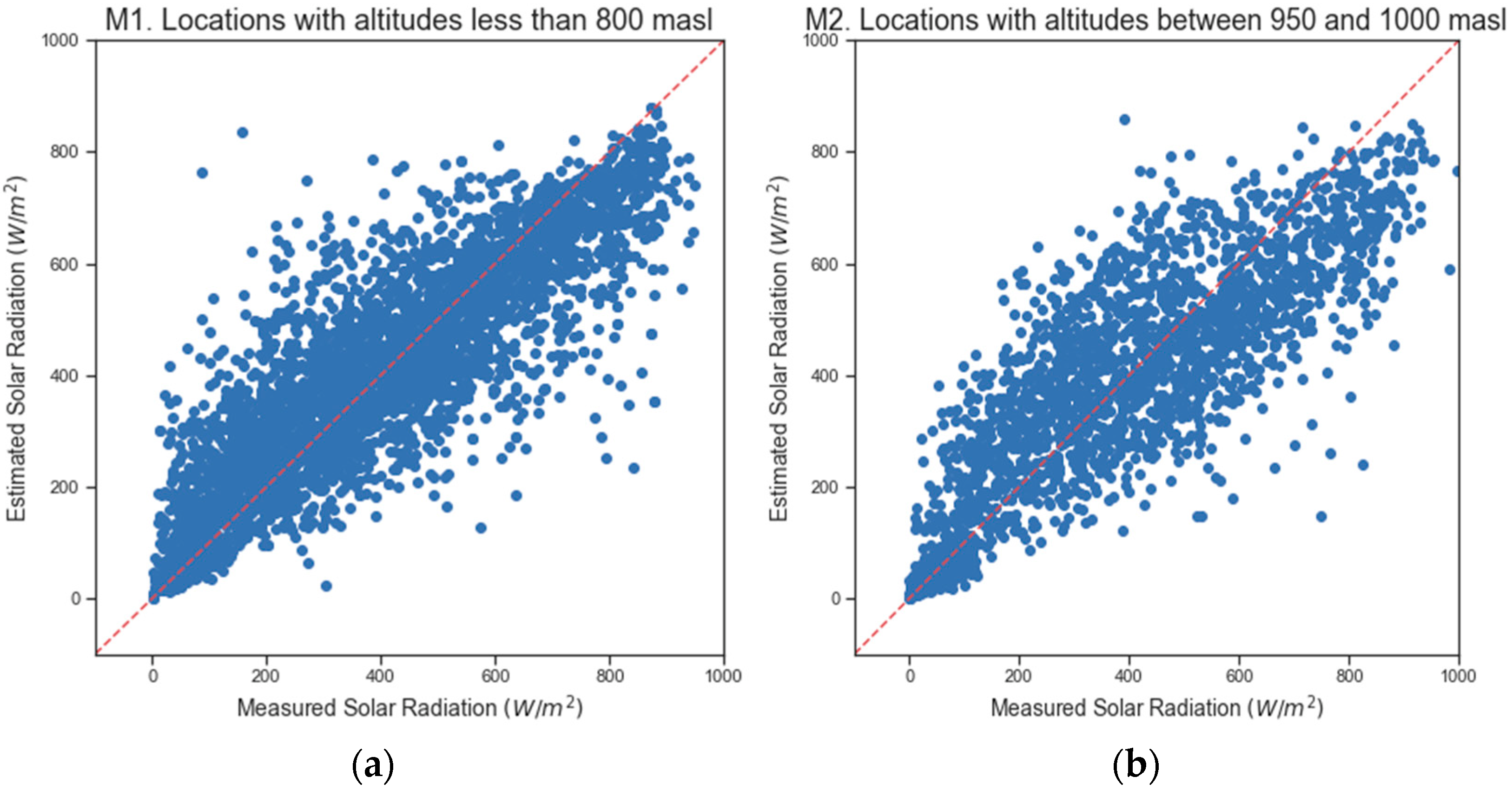
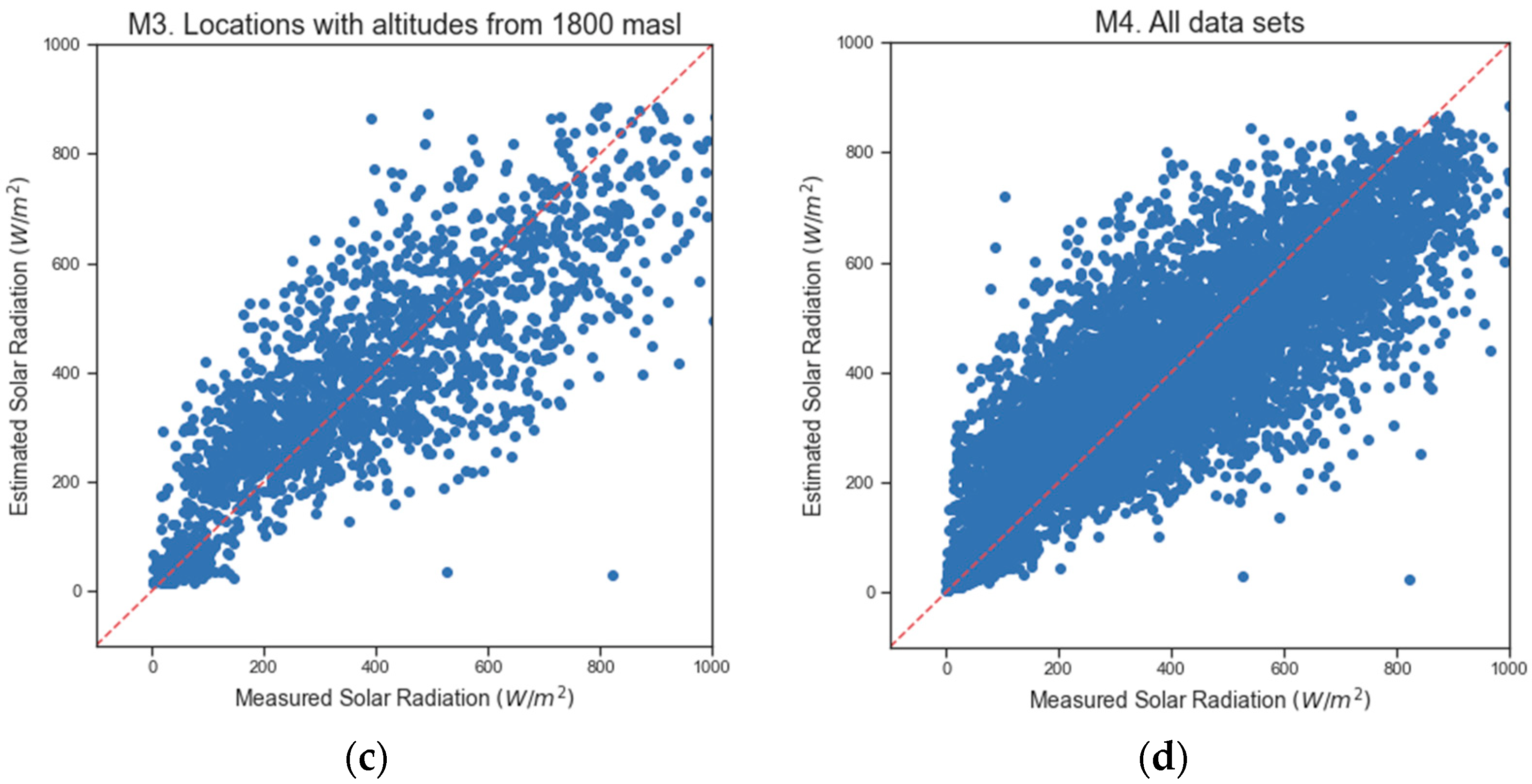
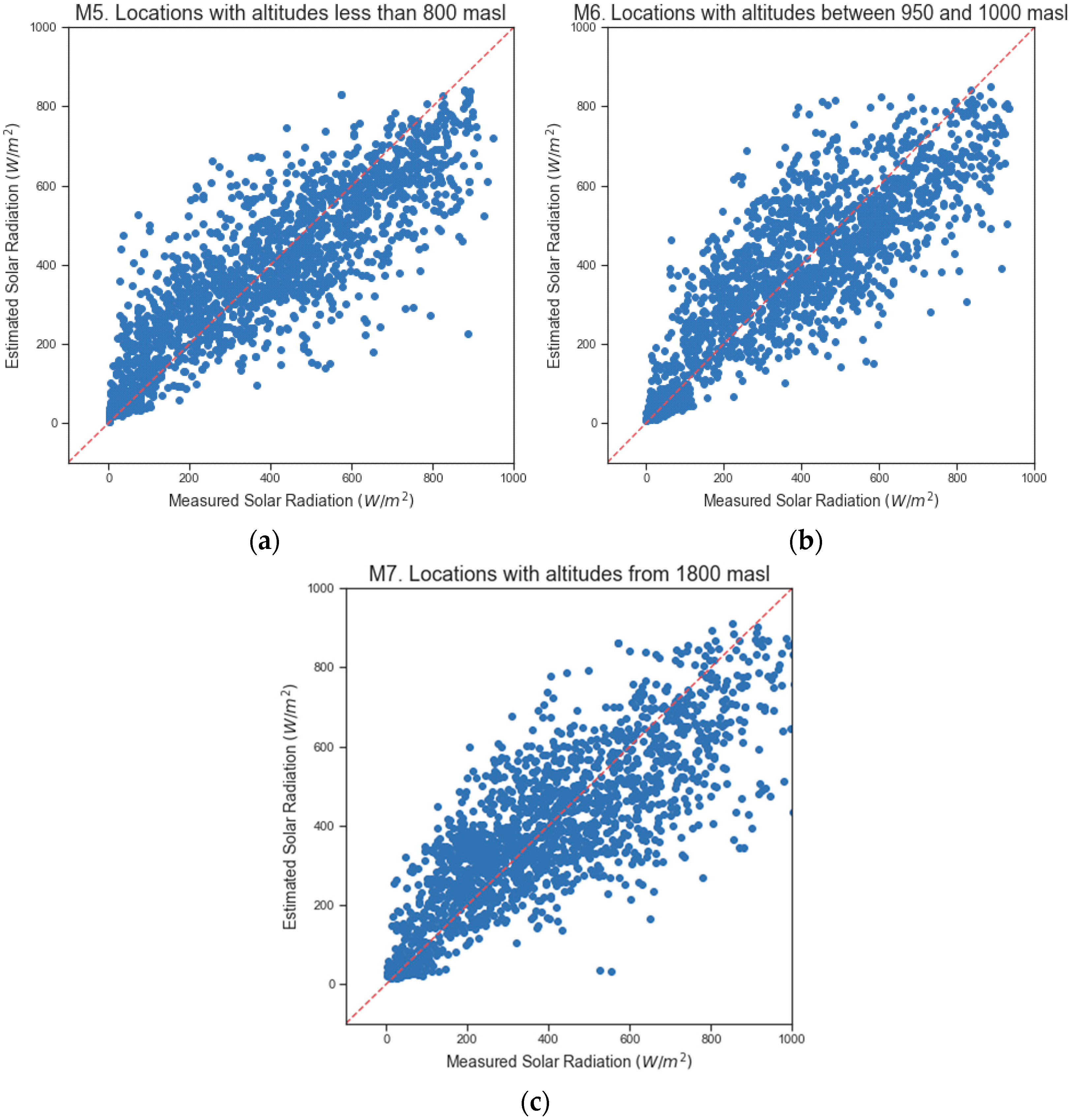
Figure 2 represents the dispersion diagrams obtained with RF, using the measured solar radiation and the solar radiation estimated by the models (M1–M3) that included 100% of the samples. The model (M1) with altitudes below 800 m.a.s.l fit the data better and showed less variability around the mean. Figure 3 shows the dispersion diagrams obtained with RF, using the measured solar radiation and the solar radiation estimated by the models (M5–M7) that used 6500 instances. Equally, the model (M5) with altitudes below 800 m.a.s.l fit the data better and showed less variability around the mean.

The Random Forest algorithm of the M1 model was experimented with. The algorithm achieved the highest results in R² (0.82) and was trained with 70% of the data with altitudes lower than 800 m.a.s.l. Subsequently, the characteristics (reflectance, cloudiness index, number of daily sunshine hours, and solar radiation at the edge of the atmosphere) were extracted from the 2014 satellite images (1965 records) in the coordinates of latitude 0.838972222 and longitude −76.57044444.

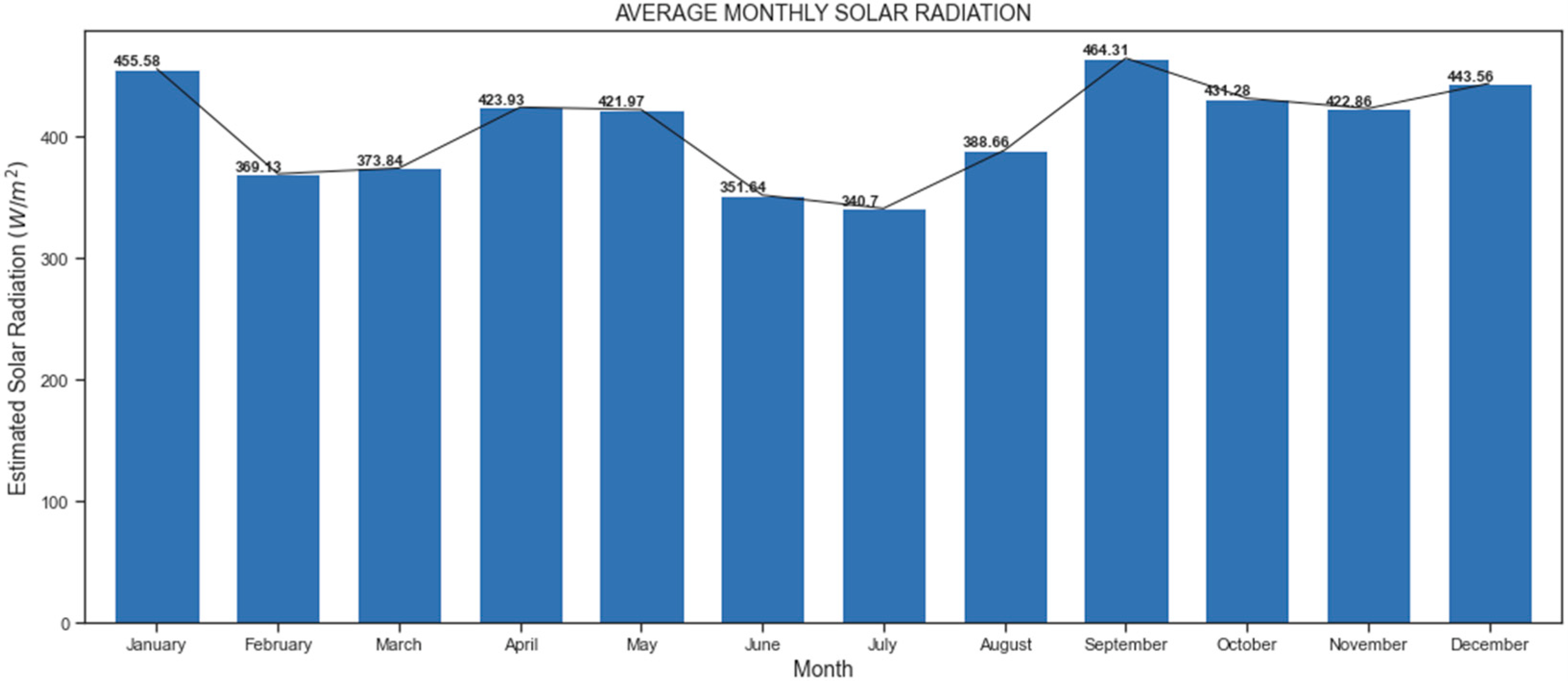
The coordinates correspond to Puerto Umbría in the department of Putumayo. It is important to point out that there is an IDEAM observation station in that place; however, it does not have solar radiation measurement sensors. The algorithm trained with the data from the M1 model; it made predictions of solar radiation in that location, and the monthly averages between 8 and 16 h can be seen in Figure 4. In this case, it is impossible to calculate the evaluation metrics of the predictions, because there are no data on the solar radiation observed on the ground.

4. Discussion

In the work in progress by Ordoñez-Palacios et al. [28], three models were evaluated for the prediction of solar radiation. The model with the best performance integrated two dimensions of information, namely, meteorological data and satellite imagery. However, it was proposed for future work to evaluate the solar radiation prediction model using images from locations with diverse altitudes above sea level, with the aim of verifying if the altitude impacts the forecast precision.

Although this work shows an inversely proportional relation between altitude and performance, it is necessary to analyze data from more monitoring stations at different altitudes and create more categories of altitude above sea level to confirm this theory.

In accordance with our work in progress, the integration of meteorological data with features extracted from satellite images allows one to achieve the best prediction in comparison to models that use each data dimension independently, although, to evaluate the performance of the algorithms, it is necessary to consider diverse data observed on the ground.

Although the level of error of the algorithms used in this research study is in a range of divergence (between 20% and 25%), it is considered reasonable for dimensioning photovoltaic systems and the prediction of power generation.

5. Conclusions

This paper evaluates the performance of four machine learning algorithms (Multiple Linear Regression, Support Vector Regression, Random Forest, and Neural Network) in predicting solar radiation in regions of Colombia located at different altitudes above sea level. The research study uses images obtained by the GOES-13 satellite in 2012, 2013, and 2014, as well as solar radiation data sets obtained by the DAGMA and IDEAM stations in the departments of Putumayo, Caquetá, Nariño, Cauca, and Valle del Cauca.

The extracting of features of the satellite images began with the request and download of the images from the NOOA website. Later, they were processed with the WCT tool, and python and a mathematical model were used to build the data sets (see Section 2.2). The highest performance was obtained by the Random Forest algorithm, followed by the Neural Network algorithm (see Table 7). The results of the performance of the models (M5–M7) that used a sample of 6500 records are shown in Table 7. The evaluation metrics used by the models are presented in Section 2.5. The influence of altitude on the results obtained by the prediction models is analyzed in Section 3 and Section 4.

According to the RF results, the model (M1) that used all the solar radiation data at altitudes below 800 m.a.s.l achieved 9% more precision in R² with respect to the model (M3) with lower performance (locations above 1800 m.a.s.l). Similarly, in terms of the root mean square error, RF achieved an error of 22 fewer points. For models (M5–M7) using a sample of 6500 records, the first model (M5) was 6% more accurate than the worst model (M7), based on R² and RMSE, with an error of approximately 20 fewer points.

The non-existence of images provided by the GOES-13 satellite on certain days of the year and at certain times of the day led to an acceptable performance of the results obtained by the automatic learning algorithms, considering that, in 2012, only 41.8% of the images between 6 am and 6 pm were available; in 2013, 39.3%; and in 2014, 41.4% (see Table 1). This loss of information led to the elimination of samples in the solar radiation data sets to enable integration with the features obtained from the images.

The most representative evaluation metrics in this work were R² and RMSE, because they exposed a trend in the models that used data from different altitudes above sea level. In the case of R², the performance of SVR, RF, and ANN deteriorates as the altitude increases. Equally, regarding RMSE, the error also increases in each model when the altitude increases. This trend can also be noted if the MAPE statistic is considered; however, the behavior of the MBE metric is random.