
Down-Hole Electromagnetic Heating of Deep Aquifers for Renewable Energy Storage


Abstract
:
1. Introduction
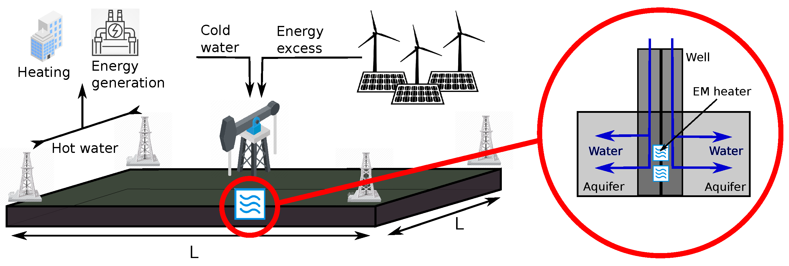
2. Physical Model
2.1. Governing Equations
2.2. EM Heating
3. Numerical Methods
4. Results and Discussion
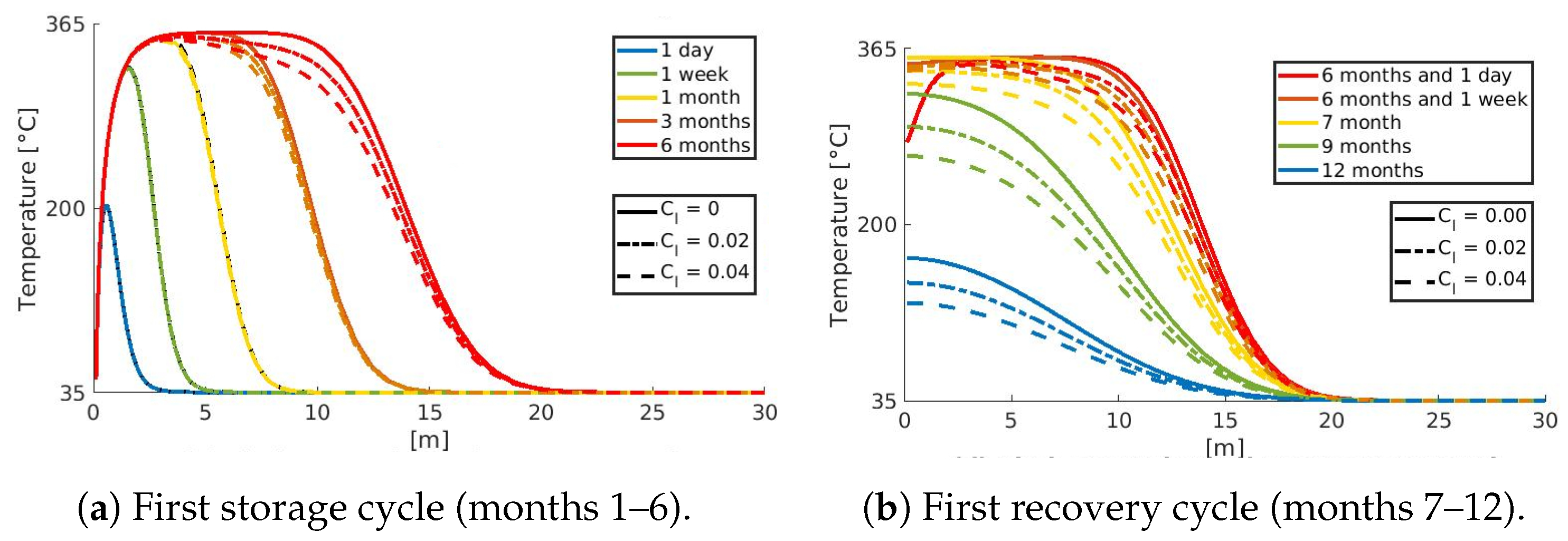
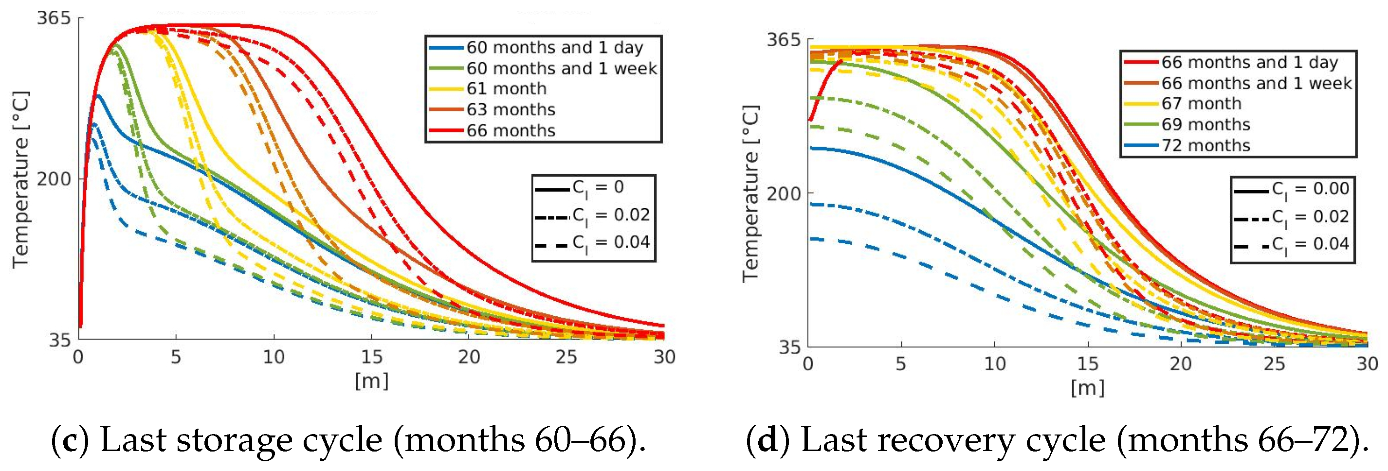
4.1. Continuous Water Injection under EM Heating
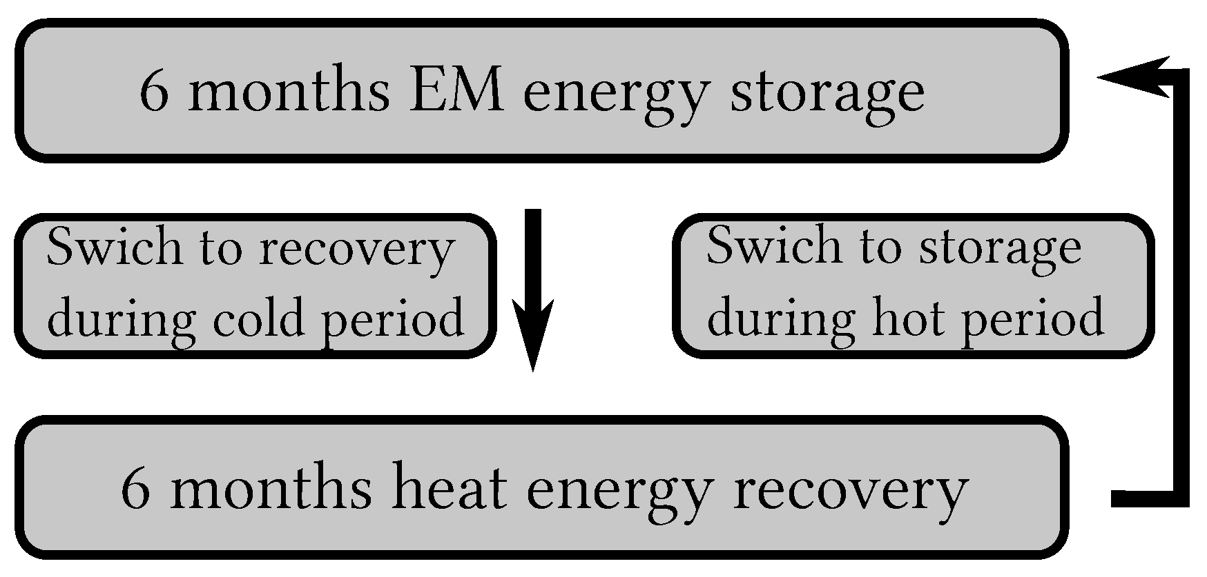
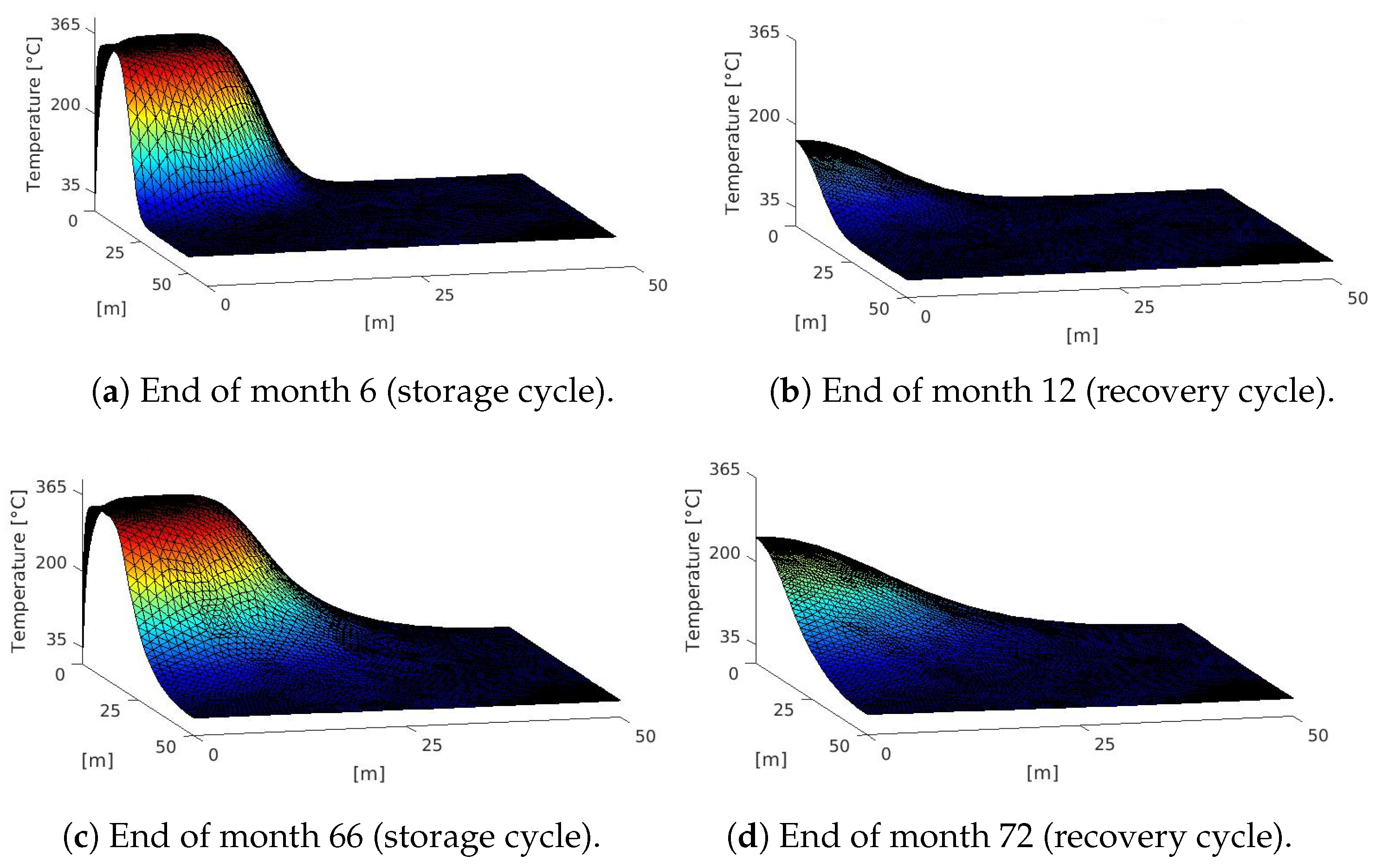
4.2. Energy Recovery
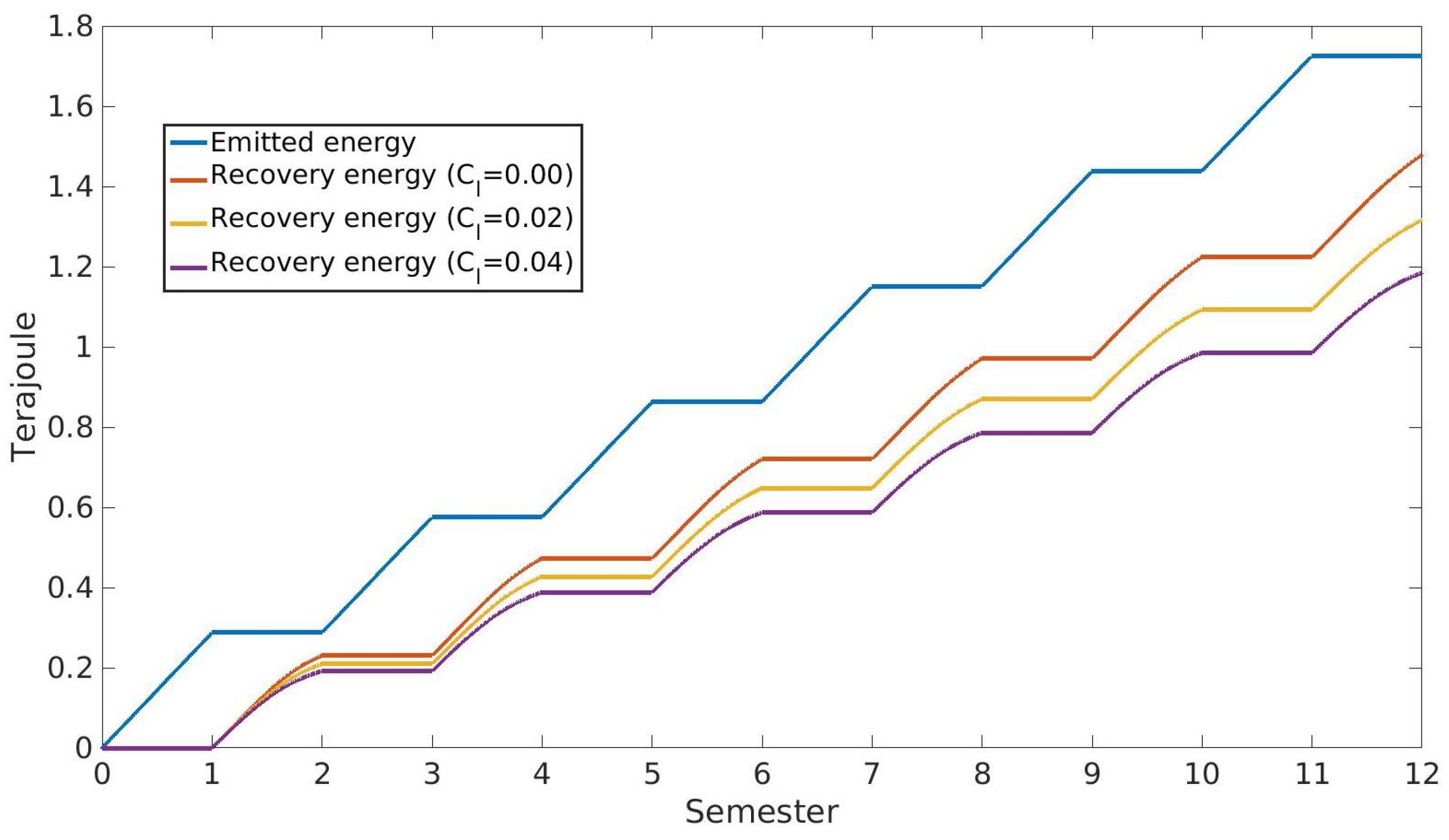
4.3. Energy Balance
4.4. Wellbore Heat Losses
5. Conclusions
- The proposed EM heating technique could be used to produce a stable thermal front, spreading the energy through the aquifer with temperatures below the boiling point.
- Our simulation results show that even considering excessive thermal losses, the EM-heating-assisted water flooding can recover up to 70% of the stored energy. In terms of efficiency, this value is also comparable with the low-temperature ATES as reported in the literature.
- The energy balance estimate in the wellbore shows that down-hole EM heating can reduce energy losses for the deep aquifers (>1000 m), which can be notable if the water is heated at the surface.
Author Contributions
Funding
Institutional Review Board Statement
Informed Consent Statement
Data Availability Statement
Acknowledgments
Conflicts of Interest
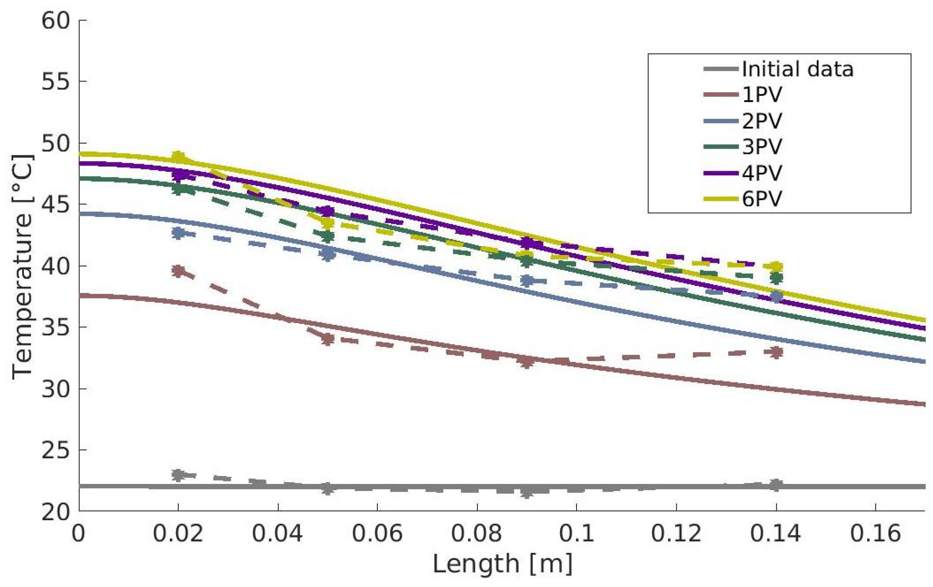
Appendix A. Model Validation

| Symbol | Physical Quantity | Exp A | Exp B | Unit (SI) |
|---|---|---|---|---|
| L | Reservoir length | [m] | ||
| A | Cross-section area | [m2] | ||
| Initial temperature | [K] | |||
| EM energy absorption | [1/m] | |||
| P | EM emitters power | 45 | 40 | [W] |
| D | Darcy velocity | 0 | [m/s] | |
| System specific heat | [MJ/m3·K] | |||
| Total fluid specific heat | [MJ/m3·K] | |||
| Total system thermal conduc. | [W/m·K] | |||
| Thermal losses coefficient | [MJ/m3·K] |

References
- Dorsey-Palmateer, R. Effects of wind power intermittency on generation and emissions. Electr. J. 2019, 32, 25–30. [Google Scholar] [CrossRef]
- Dickinson, J.S.; Buik, N.; Matthews, M.C.; Snijders, A. Aquifer thermal energy storage: Theoretical and operational analysis. Géotechnique 2009, 59, 249–260. [Google Scholar] [CrossRef]
- Sommer, W. Modelling and Monitoring of Aquifer Thermal Energy Storage: Impacts of Soil Heterogeneity, Thermal Interference and Bioremediation. Ph.D. Thesis, Wageningen University, Wageningen, The Netherlands, 2015. [Google Scholar]
- Kallesøe, A.; Vangkilde-Pedersen, T. HEATSTORE–Underground Thermal Energy Storage (UTES)-State of the Art, Example Cases and Lessons Learned. In Proceedings of the World Geothermal Congress, Reykjavik, Iceland, 24–27 October 2020. [Google Scholar]
- Fleuchaus, P.; Schüppler, S.; Bloemendal, M.; Guglielmetti, L.; Opel, O.; Blum, P. Risk analysis of High-Temperature Aquifer Thermal Energy Storage (HT-ATES). Renew. Sustain. Energy Rev. 2020, 133, 110153. [Google Scholar] [CrossRef]
- Kastner, O.; Norden, B.; Klapperer, S.; Park, S.; Urpi, L.; Cacace, M.; Blöcher, G. Thermal solar energy storage in Jurassic aquifers in Northeastern Germany: A simulation study. Renew. Energy 2017, 104, 290–306. [Google Scholar] [CrossRef]
- Schmidt, T.; Müller-Steinhagen, H. Die solar unterstützte Nahwärmeversorgung mit saisonalem Aquifer-Wärmespeicher in Rostock-Ergebnisse nach vier Betriebsjahren. In Symposium Erdgekoppelte Wärmepumpen; Geothermische Fachtagung: Landau, Germany, 2004. [Google Scholar]
- Kangas, M.; Lund, P. Modeling and simulation of aquifer storage energy systems. Sol. Energy 1994, 53, 237–247. [Google Scholar] [CrossRef]
- Ghaebi, H.; Bahadori, M.; Saidi, M. Performance analysis and parametric study of thermal energy storage in an aquifer coupled with a heat pump and solar collectors, for a residential complex in Tehran, Iran. Appl. Therm. Eng. 2014, 62, 156–170. [Google Scholar] [CrossRef]
- Badakhshan, S.; Hajibandeh, N.; Shafie-khah, M.; Catalão, J. Impact of solar energy on the integrated operation of electricity-gas grids. Energy 2019, 183, 844–853. [Google Scholar] [CrossRef]
- Lau, D.; Song, N.; Hall, C.; Jiang, Y.; Lim, S.; Perez-Wurfl, I.; Ouyang, Z.; Lennon, A. Hybrid solar energy harvesting and storage devices: The promises and challenges. Mater. Today Energy 2019, 13, 22–44. [Google Scholar] [CrossRef]
- Wilberforce, T.; Baroutaji, A.; El Hassan, Z.; Thompson, J.; Soudan, B.; Olabi, A.G. Prospects and challenges of concentrated solar photovoltaics and enhanced geothermal energy technologies. Sci. Total Environ. 2019, 659, 851–861. [Google Scholar] [CrossRef] [Green Version]
- Bera, A.; Babadagli, T. Status of electromagnetic heating for enhanced heavy oil/bitumen recovery and future prospects: A review. Appl. Energy 2015, 151, 206–226. [Google Scholar] [CrossRef]
- Shafiai, S.; Gohari, A. Conventional and electrical EOR review: The development trend of ultrasonic application in EOR. J. Pet. Explor. Prod. Technol. 2020, 10, 2923–2945. [Google Scholar] [CrossRef]
- Sivakumar, P.; Krishna, S.; Hari, S.; Vij, R. Electromagnetic heating, an eco-friendly method to enhance heavy oil production: A review of recent advancements. Environ. Technol. Innov. 2020, 20, 101100. [Google Scholar] [CrossRef]
- Hasanvand, M.Z.; Golparvar, A. A Critical Review of Improved Oil Recovery by Electromagnetic Heating. Pet. Sci. Technol. 2014, 32, 631–637. [Google Scholar] [CrossRef]
- Pizarro, J.; Trevisan, O. Electrical heating of oil reservoirs: Numerical simulation and field test results. J. Pet. Technol. 1990, 42, 1–320. [Google Scholar] [CrossRef]
- Sahni, A.; Kumar, M.; Knapp, R.B. Electromagnetic heating methods for heavy oil reservoirs. In Proceedings of the Western Regional Meeting, SPE/AAPG, Long Beach, CA, USA, 19–23 June 2000; pp. 19–23. [Google Scholar]
- Chhetri, A.; Islam, M. A critical review of electromagnetic heating for enhanced oil recovery. Pet. Sci. Technol. 2008, 26, 1619–1631. [Google Scholar] [CrossRef]
- Paz, P.; Hollmann, T.; Kermen, E.; Chapiro, G.; Slob, E.; Zitha, P. EM Heating-Stimulated Water Flooding for Medium–Heavy Oil Recovery. Transp. Porous Media 2017, 119, 57–75. [Google Scholar] [CrossRef] [Green Version]
- Cerutti, A.; Bandinelli, M.; Bientinesi, M.; Petarca, L.; De Simoni, M.; Manotti, M.; Maddinelli, G. A New Technique for Heavy Oil Recovery Based on Electromagnetic Heating: System Design and Numerical Modelling. Chem. Eng. Trans. 2013, 32, 1255–1260. [Google Scholar]
- Jha, A.K.; Joshi, N.; Singh, A. Applicability and Assessment of Micro-Wave Assisted Gravity Drainage (MWAGD) Applications in Mehsana Heavy Oil Field. In Proceedings of the SPE Heavy Oil Conference and Exhibition, Kuwait City, Kuwait, 12–14 December 2011; pp. 11–14. [Google Scholar]
- Mukhametshina, A.; Martynov, E. Electromagnetic Heating of Heavy Oil and Bitumen: A Review of Experimental Studies and Field Applications. J. Pet. Eng. 2013, 2013, 476519. [Google Scholar] [CrossRef]
- Eskandari, S.; Jalalalhosseini, S.M.; Mortezazadeh, E. Microwave Heating as an Enhanced Oil Recovery Method—Potentials and Effective Parameters. Energy Sources Part A Recovery Util. Environ. Eff. 2015, 37, 742–749. [Google Scholar] [CrossRef]
- Soliman, M. Approximate solutions for flow of oil heated using microwaves. J. Pet. Sci. Eng. 1997, 18, 93–100. [Google Scholar] [CrossRef]
- Rubinstein, L. The total heat losses in injection of hot liquid Into a stratum. Neft. Gaz 1959, 9, 41. [Google Scholar]
- Carrizales, M.A.; Lake, L.W.; Johns, R.T. Multiphase fluid flow simulation of heavy oil recovery by electromagnetic heating. In SPE IOR Symposium; OnePetro: Richardson, TX, USA, 2010. [Google Scholar]
- Almeida, S.O.; Zitha, P.L.J.; Chapiro, G. A method for analyzing electromagnetic heating assisted water flooding process for heavy oil recovery. Transp. Porous Media 2021. [Google Scholar] [CrossRef]
- Fanchi, J.R. Feasibility of reservoir heating by electromagnetic irradiation. In Proceedings of the SPE Annual Technical Conference and Exhibition, New Orleans, LA, USA, 23–26 September 1990. [Google Scholar]
- Darcy, H. Les Fontaines Publiques de la Ville de Dijon; Victor Dalmond: Paris, France, 1856. [Google Scholar]
- Whitaker, S. The equations of motion in porous media. Chem. Eng. Sci. 1966, 21, 291–300. [Google Scholar] [CrossRef]
- Viswanath, D.; Ghosh, T.; Prasad, D.; Dutt, N.; Rani, K. Viscosity of Liquids: Theory, Estimation, Experiment, and Data; Springer: Dordrecht, The Netherlands, 2007. [Google Scholar]
- Chen, Z.; Huan, G.; Ma, Y. Computational Methods for Multiphase Flows in Porous Media (Computational Science and Engineering 2); SIAM: Philadelphia, PA, USA, 2006. [Google Scholar]
- Kaviany, M. Principles of Heat Transfer in Porous Media; Springer: Berlin/Heidelberg, Germany, 1991. [Google Scholar]
- Sudiko, M. Elementes of Electromagnetics; Oxford University Press: New York, NY, USA, 2014. [Google Scholar]
- Stratton, J.A. Electromagnetic Theory; McGraw-Hill: New York, NY, USA, 1941. [Google Scholar]
- Hughes, T.; Franca, P.; Hulbert, G. A new finite element formulation for computational fluid dynamics: VIII. The galerkin/least-squares method for advective-diffusive equations. Comput. Methods Appl. Mech. Eng. 1989, 73, 173–189. [Google Scholar] [CrossRef]
- Settari, A.; Walters, D. Advances in Coupled Geomechanical and Reservoir Modeling with Applications to Reservoir Compaction. SPE J. 2001, 6, 334–342. [Google Scholar] [CrossRef]
- Ramey, H.J., Jr. Wellbore Heat Transmission. J. Pet. Technol. 1962, 14, 427–435. [Google Scholar] [CrossRef]
- Willhite, G. Over-All Heat Transfer Coefficients in Steam And Hot Water Injection Wells. J. Pet. Technol. 1967, 19, 607–615. [Google Scholar] [CrossRef]
- Cheng, W.L.; Han, B.B.; Nian, Y.L.; Wang, C.L. Study on wellbore heat loss during hot water with multiple fluids injection in offshore well. Appl. Therm. Eng. 2016, 95, 247–263. [Google Scholar] [CrossRef]
- Ameli, F.; Alashkar, A.; Hemmati-Sarapardeh, A. Thermal Recovery Processes; Elsevier: Amsterdam, The Netherlands, 2018; pp. 139–186. [Google Scholar]
- Fan, Z.; Parashar, R. Analytical Solutions for a Wellbore Subjected to a Non-isothermal Fluid Flux: Implications for Optimizing Injection Rates, Fracture Reactivation, and EGS Hydraulic Stimulation. Rock Mech. Rock Eng. 2019, 52, 4715–4729. [Google Scholar] [CrossRef]
- Fan, Z.; Parashar, R.; Jin, Z.H. Impact of convective cooling on pore pressure and stresses around a borehole subjected to a constant flux: Implications for hydraulic tests in an enhanced geothermal system reservoir. Interpretation 2020, 8, SG13–SG20. [Google Scholar] [CrossRef]
| Symbol | Physical Quantity | Value | Unit (SI) |
|---|---|---|---|
| porosity | 0.220 | [-] | |
| water saturation | 1 | [-] | |
| water viscosity | [Pa·s] | ||
| porous media density | [Kg/m3] | ||
| water density | [Kg/m3] | ||
| PM specific heat capacity | [J/Kg·K] | ||
| water specific heat capacity | [J/Kg·K] | ||
| PM thermal conductivity | 2.30 | [W/m·K] | |
| water thermal conductivity | 0.58 | [W/m·K] | |
| L | reservoir length and width | 100 | [m] |
| flux rate | [m/s] | ||
| A | cross section | 1.7 | [m2] |
| h | reservoir height | 5 | [m] |
| P | power of the EM emitter | 18.5 | [kW] |
| initial temperature | 308.15 | [K] | |
| k | permeability | 700 | [mD] |
| constant Equation (1) | −4.53 | [-] | |
| constant Equation (1) | −220.53 | [-] | |
| constant Equation (1) | 149.39 | [-] | |
| vacuum electric permittivity | [F/m] | ||
| relative electric permittivity | 81 | [F/m] | |
| vacuum magnetic permeability | [H/m] | ||
| relative magnetic permeability | 1 | [H/m] | |
| medium conductivity | 0.02 | [S/m] | |
| angular frequency | [rad/s] | ||
| water EM energy absorption | [1/m] | ||
| system specific heat | 2.822 | [MJ/m3·K] | |
| total fluid specific heat | 6.625 | [MJ/m3·K] | |
| tot. system thermal conductivity | 1.9216 | [W/m·K] | |
| thermal losses | 0.02 | [W/m3·K] |
| Yr. | Rec. | R. St. | Lost | Rec. | R. St. | Lost | Rec. | R. St. | Lost |
|---|---|---|---|---|---|---|---|---|---|
| 1 | 81.1% | 18.9% | 0% | 73.8% | 15.5% | 10.7% | 67.4% | 12.7% | 19.9% |
| 2 | 83.2% | 16.8% | 0% | 75.2% | 12.6% | 12.2% | 68.3% | 9.6% | 22.1% |
| 3 | 84.5% | 15.5% | 0% | 76.0% | 10.7% | 13.3% | 68.8% | 7.6% | 23.6% |
| 4 | 85.5% | 14.5% | 0% | 76.6% | 9.2% | 14.2% | 69.2% | 6.2% | 24.6% |
| 5 | 86.2% | 13.8% | 0% | 76.9% | 8.1% | 15.0% | 69.4% | 5.2% | 25.4% |
| 6 | 86.8% | 13.2% | 0% | 77.3% | 7.2% | 15.5% | 69.5% | 4.5% | 26.0% |
| Diameters [in] | Th. Conductivity [W/m.K] | Depth [m] | Heat Losses % | ||
|---|---|---|---|---|---|
| 5 | 7 3/5 | 1.4 | 0.2 | 1000 | 1.47 |
| 7 3/5 | 9 3/4 | 1.4 | 0.2 | 1000 | 2.18 |
| 9 3/4 | 20 | 2.8 | 0.4 | 2000 | 2.35 |
| 5 | 7 3/5 | 2.8 | 0.4 | 2000 | 5.90 |
| 9 3/4 | 12 | 1.4 | 0.2 | 1000 | 8.85 |
| 9 3/4 | 12 | 2.8 | 0.4 | 2000 | 10.6 |
Publisher’s Note: MDPI stays neutral with regard to jurisdictional claims in published maps and institutional affiliations. |
© 2022 by the authors. Licensee MDPI, Basel, Switzerland. This article is an open access article distributed under the terms and conditions of the Creative Commons Attribution (CC BY) license (https://creativecommons.org/licenses/by/4.0/).
Share and Cite
Almeida, S.O.d.; Chapiro, G.; Zitha, P.L.J. Down-Hole Electromagnetic Heating of Deep Aquifers for Renewable Energy Storage. Energies 2022, 15, 3982. https://doi.org/10.3390/en15113982
Almeida SOd, Chapiro G, Zitha PLJ. Down-Hole Electromagnetic Heating of Deep Aquifers for Renewable Energy Storage. Energies. 2022; 15(11):3982. https://doi.org/10.3390/en15113982
Chicago/Turabian StyleAlmeida, Samuel O. de, Grigori Chapiro, and Pacelli L. J. Zitha. 2022. "Down-Hole Electromagnetic Heating of Deep Aquifers for Renewable Energy Storage" Energies 15, no. 11: 3982. https://doi.org/10.3390/en15113982
APA StyleAlmeida, S. O. d., Chapiro, G., & Zitha, P. L. J. (2022). Down-Hole Electromagnetic Heating of Deep Aquifers for Renewable Energy Storage. Energies, 15(11), 3982. https://doi.org/10.3390/en15113982