
Greedy Sine-Cosine Non-Hierarchical Grey Wolf Optimizer for Solving Non-Convex Economic Load Dispatch Problems


Abstract
:1. Introduction
2. Formulation of ELD Problem
2.1. Cost Function
2.2. Constraints of the Problem
2.2.1. Power Balance
2.2.2. Active Power Limit
2.2.3. Prohibit Operating Zones (POZs)
2.2.4. Ramp Rate Limit
3. The Proposed Algorithm
3.1. GWO Algorithm
3.1.1. Social Hierarchy of the Grey Wolves
3.1.2. Encircling Strategy
3.1.3. Hunting Strategy
3.1.4. Attacking Strategy (Exploitation Phase)
3.1.5. Searching for Prey (Exploration Phase)
3.2. Nonhierarchical GWO (NHGWO)
3.3. Greedy Sine-Cosine Non-Hierarchical Grey Wolf Optimizer (G-SCNHGWO)
| Algorithm 1: Pseudocode of G-SCNHGWO algorithm. |
| G-SCNHGWO: |
| Generate initial grey wolves(i = 1, 2, …, Npop); Set the initial value of parameters a,and; Evaluate the objective value of the initial population; Initial fitness evolution of grey wolves and save the local position best for any gray wolf; Set t = 1; While (t < maximum value of iterations) For (each member ith) Update their current position using Equations (17), (18), (21) and (22); end for Update parameters a,,; Evaluate the objective value of all searching agents members; Update the value of grey wolves and save the best position for any gray wolf; Set t = t + 1; end while returnas the best solution. |
3.4. Application of G-SCNHGWO in ELD Problem
- Step (1) Set the parameters of G-SCNHGWO, the maximum number of iterations (itermax), the population size of grey wolves (Npop), B-coefficients, and data of the generation units.
- Step (2) Generate grey wolves.
- Step (3) Calculate the cost function for each member in the initial population. The penalty factors (big positive numbers) are used to transform the optimization problem with constraints into a problem with no constraints [32]. The value of penalty factors is determined experimentally for each problem and must be chosen to satisfy the associated constraint.
- Step (4) Use G-SCNHGWO phases to update the obtained solutions.
- Step (5) Calculate the value of for new solutions.
- Step (6) Update α, β, and δ wolves by comparing the old and new solutions.
- Step (7) If the termination criterion (itermax) is not satisfied, go to Step 4.
4. Simulation Results
- Case A-type 1: A test system with ten thermal units, a demand of 2700 MW, with MF constraints, and neglecting transmission power loss [35].
- Case A-type 2: Similar to Case A-Type 1, considering VPE constraints [35].
- Case B-type 1: A test system with 15 thermal units, a demand of 2630 MW, considering transmission power loss and POZ constraints [32].
- Case B-type 2: Similar to Case B-Type 1, considering ramp rate limits [32].
- Case C: A test system with 40 thermal units, a demand of 10,500 MW, and VPE constraints [65].
- Case D: A large-scale test system with 140 thermal units, a demand of 49,342 MW, and considering VPE and POZ constraints [80].
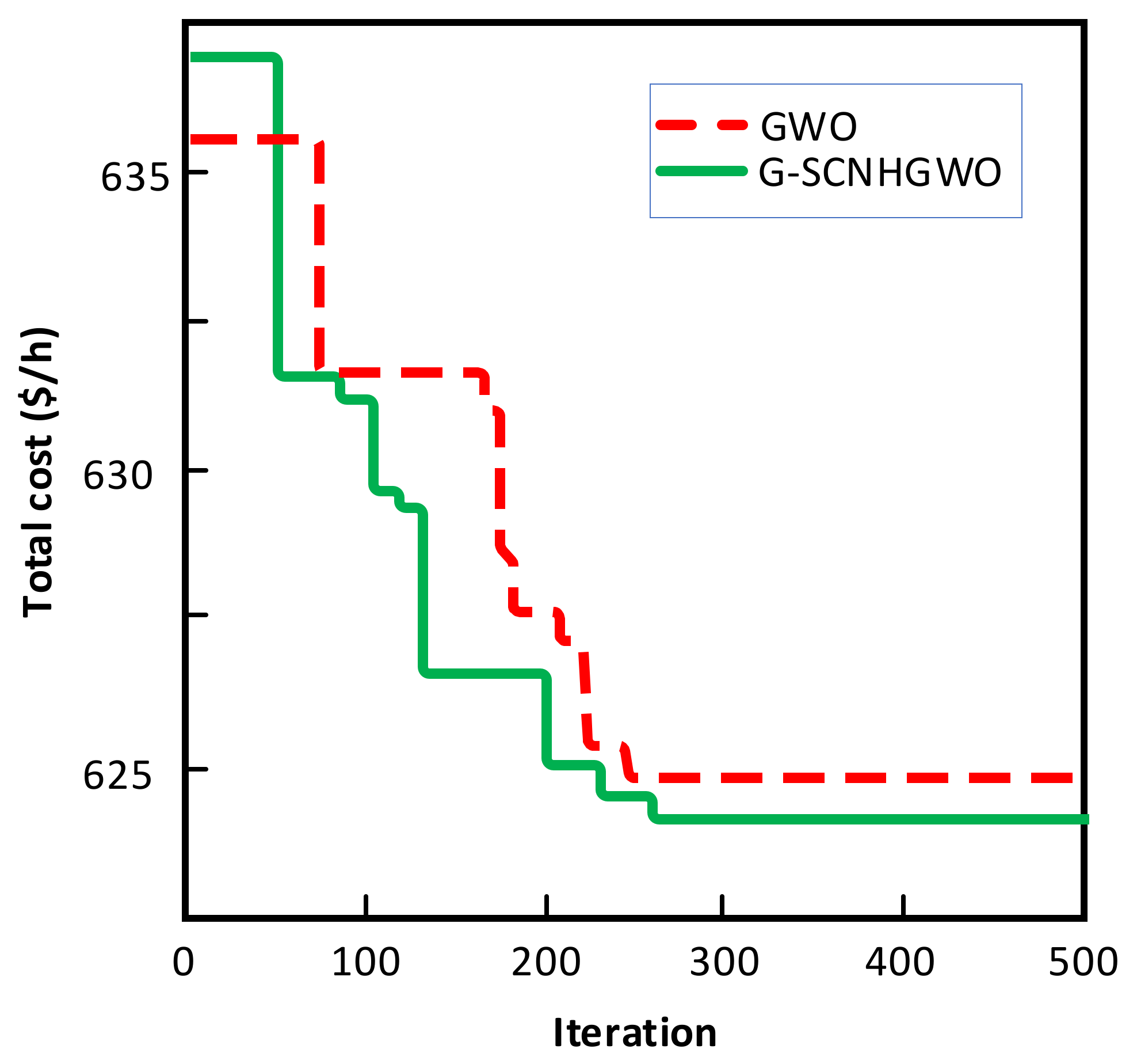
4.1. CASE A: A Test System with 10 Generation Units
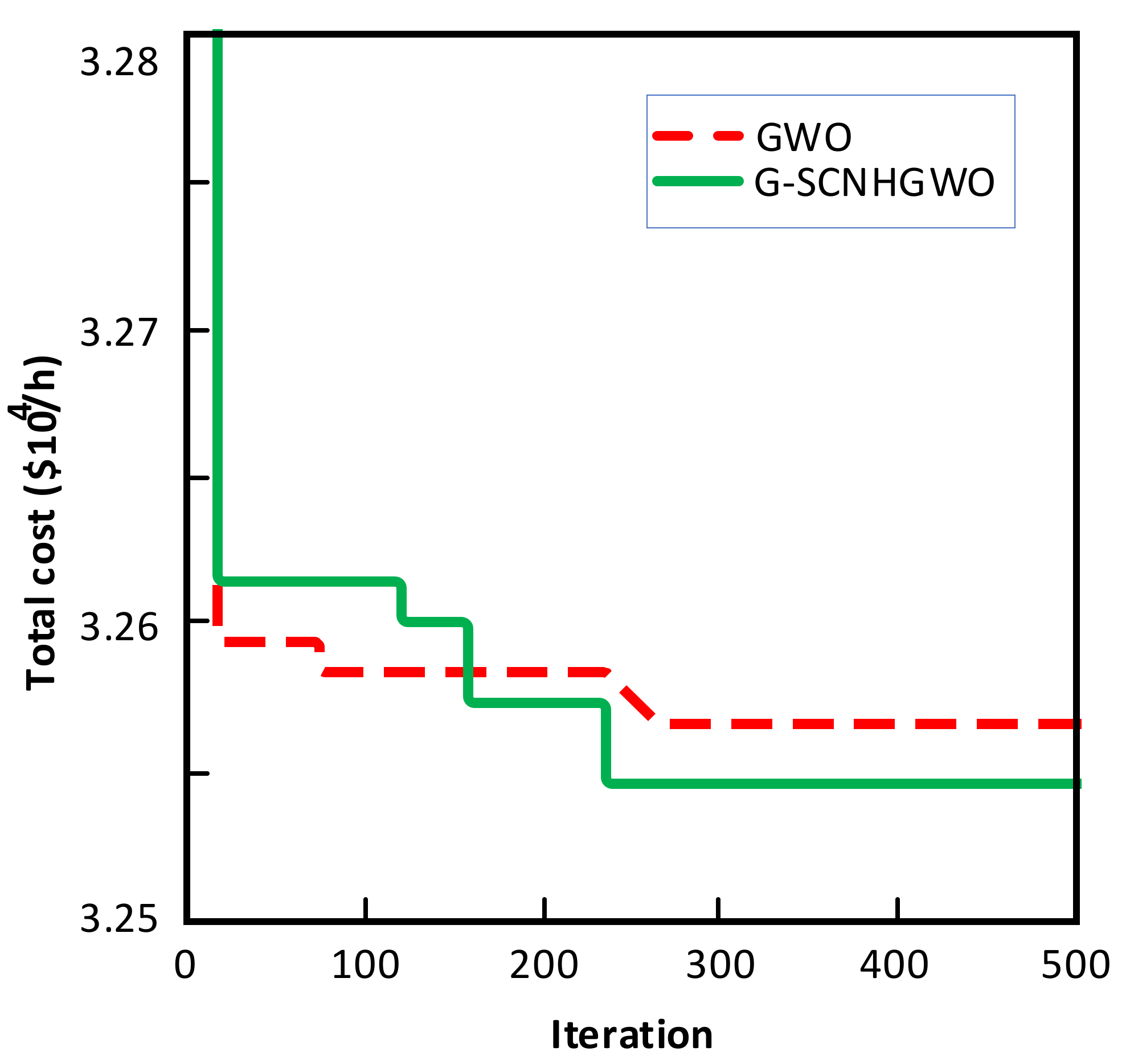
4.2. CASE B: A Test System with 15 Generation Units
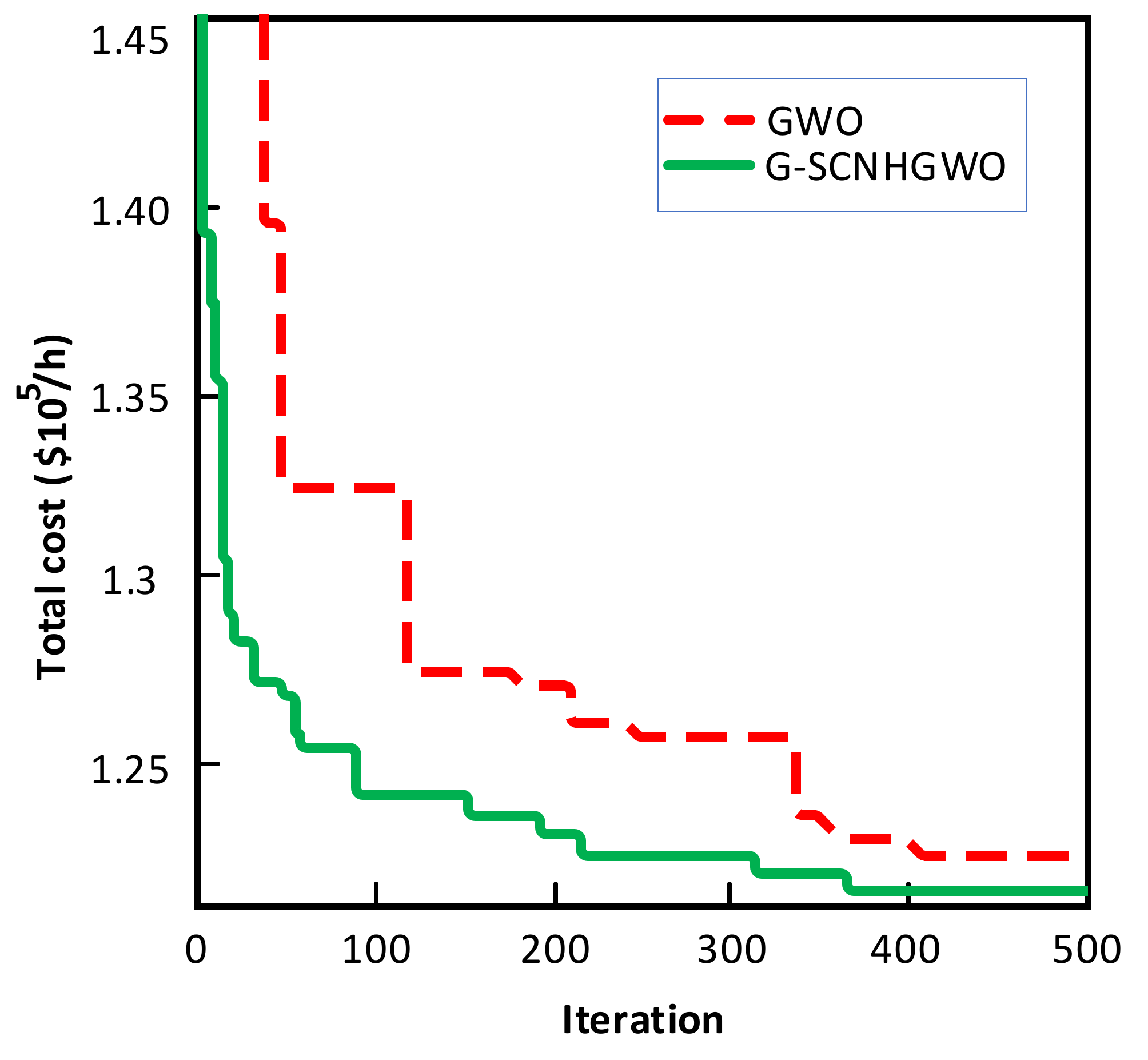
4.3. Case C: A Test System with 40 Generation Units
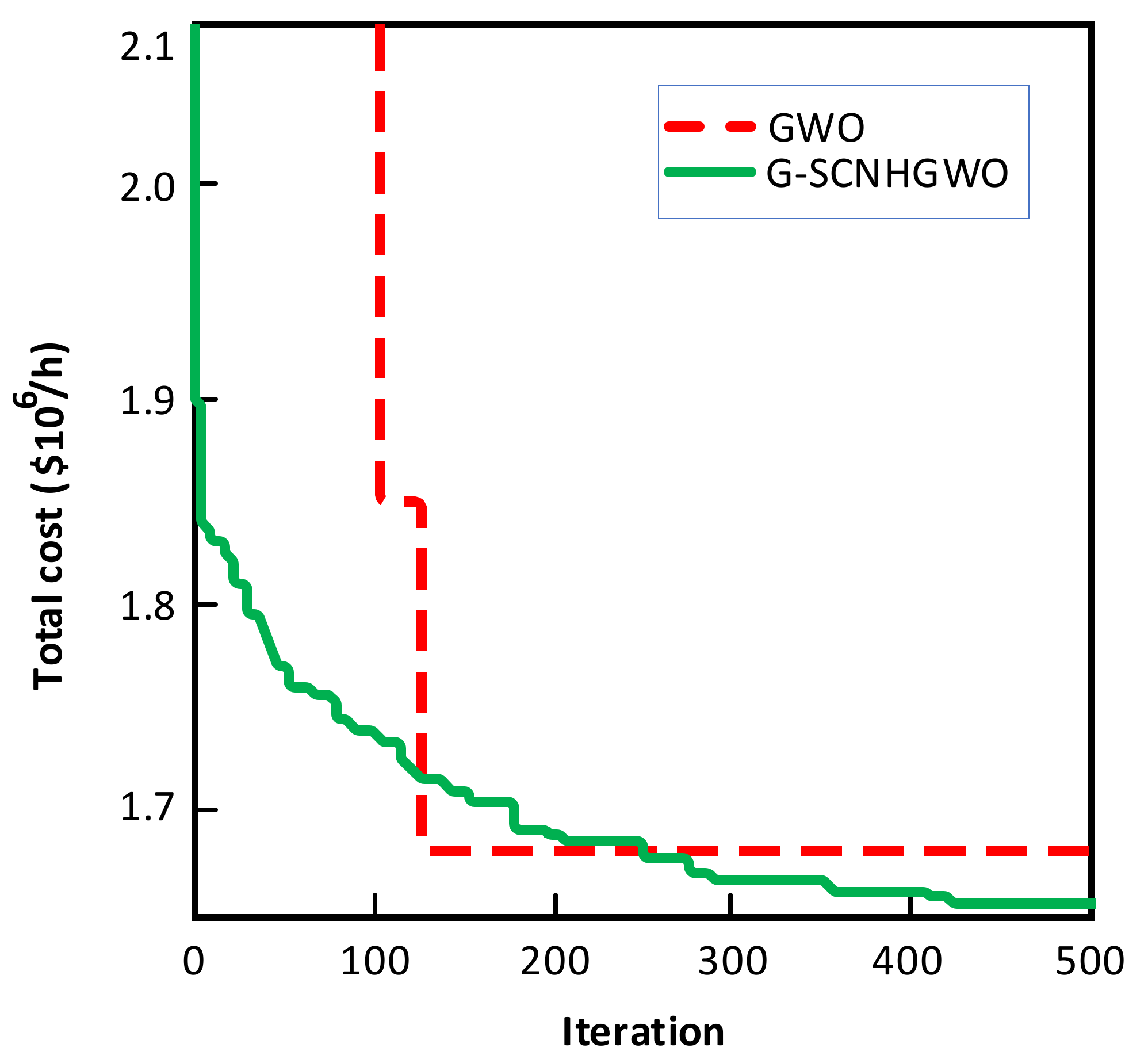
4.4. Case D: A Test System with 140 Generation Units
5. Conclusions
Author Contributions
Funding
Institutional Review Board Statement
Informed Consent Statement
Data Availability Statement
Conflicts of Interest
References
- Radosavljevic, J. Metaheuristic Optimization in Power Engineering; Institution of Engineering and Technology: London, UK, 2018. [Google Scholar] [CrossRef]
- Hemmati, R.; Wu, F.; El-Refaie, A. Survey of insulation systems in electrical machines. In Proceedings of the 2019 IEEE International Electric Machines and Drives Conference, IEMDC 2019, San Diego, CA, USA, 12–15 May 2019; pp. 2069–2076. [Google Scholar]
- Ghasemi, M. A Chaotic Modified Algorithm for Economic Dispatch Problems with Generator Constraints. Am. J. Electr. Comput. Eng. 2017, 1, 61–71. [Google Scholar]
- Basu, M. Artificial bee colony optimization for multi-area economic dispatch. Int. J. Electr. Power Energy Syst. 2013, 49, 181–187. [Google Scholar] [CrossRef]
- Aydın, D.; Özyön, S. Solution to non-convex economic dispatch problem with valve point effects by incremental artificial bee colony with local search. Appl. Soft Comput. 2013, 13, 2456–2466. [Google Scholar] [CrossRef]
- Parouha, R.P.; Verma, P. An innovative hybrid algorithm to solve nonconvex economic load dispatch problem with or without valve point effects. Int. Trans. Electr. Energy Syst. 2021, 31, e12682. [Google Scholar] [CrossRef]
- Mohammadian, M.; Lorestani, A.; Ardehali, M.M. Optimization of single and multi-areas economic dispatch problems based on evolutionary particle swarm optimization algorithm. Energy 2018, 161, 710–724. [Google Scholar] [CrossRef]
- Silva Chavez, J.C.; Zamora-Mendez, A.; Arrieta Paternina, M.R.; Yrena Heredia, J.F.; Cardenas-Javier, R. A hybrid optimization framework for the non-convex economic dispatch problem via meta-heuristic algorithms. Electr. Power Syst. Res. 2019, 177, 105999. [Google Scholar] [CrossRef]
- Suman, M.; Sakthivel, V.P. Coulomb’s and Franklin’s Laws Based Optimization for Nonconvex Economic and Emission Dispatch Problems. Int. Energy J. 2020, 20, 225–238. [Google Scholar]
- Kheshti, M.; Kang, X.; Li, J.; Regulski, P.; Terzija, V. Lightning flash algorithm for solving non-convex combined emission economic dispatch with generator constraints. IET Gener. Transm. Distrib. 2018, 12, 104–116. [Google Scholar] [CrossRef]
- Lu, H.; Sriyanyong, P.; Song, Y.H.; Dillon, T. Experimental study of a new hybrid PSO with mutation for economic dispatch with non-smooth cost function. Int. J. Electr. Power Energy Syst. 2010, 32, 921–935. [Google Scholar] [CrossRef]
- Jadoun, V.K.; Gupta, N.; Niazi, K.R.; Swarnkar, A. Modulated particle swarm optimization for economic emission dispatch. Int. J. Electr. Power Energy Syst. 2015, 73, 80–88. [Google Scholar] [CrossRef]
- Selvakumar, A.I.; Thanushkodi, K. A New Particle Swarm Optimization Solution to Nonconvex Economic Dispatch Problems. IEEE Trans. Power Syst. 2007, 22, 42–51. [Google Scholar] [CrossRef]
- Chaturvedi, K.T.; Pandit, M.; Srivastava, L. Self-Organizing Hierarchical Particle Swarm Optimization for Nonconvex Economic Dispatch. IEEE Trans. Power Syst. 2008, 23, 1079–1087. [Google Scholar] [CrossRef]
- Chen, J.; Imani Marrani, H. An Efficient New Hybrid ICA-PSO Approach for Solving Large Scale Non-convex Multi Area Economic Dispatch Problems. J. Electr. Eng. Technol. 2020, 15, 1127–1145. [Google Scholar] [CrossRef]
- Qin, Q.; Cheng, S.; Chu, X.; Lei, X.; Shi, Y. Solving non-convex/non-smooth economic load dispatch problems via an enhanced particle swarm optimization. Appl. Soft Comput. 2017, 59, 229–242. [Google Scholar] [CrossRef]
- Rajagopalan, A.; Sengoden, V.; Govindasamy, R. Solving economic load dispatch problems using chaotic self-adaptive differential harmony search algorithm. Int. Trans. Electr. Energy Syst. 2014, 25, 845–858. [Google Scholar] [CrossRef]
- Hamdi, M.; Idomghar, L.; Chaoui, M.; Kachouri, A. An improved adaptive differential evolution optimizer for non-convex Economic Dispatch Problems. Appl. Soft Comput. 2019, 85, 105868. [Google Scholar] [CrossRef]
- Neto, J.X.V.; Reynoso-Meza, G.; Ruppel, T.H.; Mariani, V.C.; dos Santos Coelho, L. Solving non-smooth economic dispatch by a new combination of continuous GRASP algorithm and differential evolution. Int. J. Electr. Power Energy Syst. 2017, 84, 13–24. [Google Scholar] [CrossRef]
- Sayah, S.; Hamouda, A. A hybrid differential evolution algorithm based on particle swarm optimization for nonconvex economic dispatch problems. Appl. Soft Comput. 2013, 13, 1608–1619. [Google Scholar] [CrossRef]
- Lohokare, M.R.; Panigrahi, B.K.; Pattnaik, S.S.; Devi, S.; Mohapatra, A. Neighborhood Search-Driven Accelerated Biogeography-Based Optimization for Optimal Load Dispatch. IEEE Trans. Syst. Man Cybern. Part C Appl. Rev. 2012, 42, 641–652. [Google Scholar] [CrossRef]
- Nee Dey, S.H. Teaching Learning Based Optimization for Different Economic Dispatch Problems. Sci. Iran. 2014, 21, 870–884. [Google Scholar]
- Alanazi, M.S. A Modified Teaching—Learning-Based Optimization for Dynamic Economic Load Dispatch Considering Both Wind Power and Load Demand Uncertainties with Operational Constraints. IEEE Access 2021, 9, 101665–101680. [Google Scholar] [CrossRef]
- He, X.; Rao, Y.; Huang, J. A novel algorithm for economic load dispatch of power systems. Neurocomputing 2016, 171, 1454–1461. [Google Scholar] [CrossRef]
- Vo, D.N.; Schegner, P.; Ongsakul, W. Cuckoo search algorithm for non-convex economic dispatch. IET Gener. Transm. Distrib. 2013, 7, 645–654. [Google Scholar] [CrossRef]
- Yu, J.; Kim, C.-H.; Rhee, S.-B. Clustering cuckoo search optimization for economic load dispatch problem. Neural Comput. Appl. 2020, 32, 16951–16969. [Google Scholar] [CrossRef]
- Azizipanah-Abarghooee, R.; Niknam, T.; Zare, M.; Gharibzadeh, M. Multi-objective short-term scheduling of thermoelectric power systems using a novel multiobjective θ-improved cuckoo optimisation algorithm. IET Gener. Transm. Distrib. 2014, 8, 873–894. [Google Scholar] [CrossRef]
- Nguyen, T.T.; Vo, D.N. The application of one rank cuckoo search algorithm for solving economic load dispatch problems. Appl. Soft Comput. 2015, 37, 763–773. [Google Scholar] [CrossRef]
- Kien, L.C.; Nguyen, T.T.; Hien, C.T.; Duong, M.Q. A Novel Social Spider Optimization Algorithm for Large-Scale Economic Load Dispatch Problem. Energies 2019, 12, 1075. [Google Scholar] [CrossRef] [Green Version]
- Elsayed, W.T.; Hegazy, Y.G.; Bendary, F.M.; El-bages, M.S. Modified social spider algorithm for solving the economic dispatch problem. Eng. Sci. Technol. Int. J. 2016, 19, 1672–1681. [Google Scholar] [CrossRef] [Green Version]
- Karimi, N.; Khandani, K. Social optimization algorithm with application to economic dispatch problem. Int. Trans. Electr. Energy Syst. 2020, 30, e12593. [Google Scholar] [CrossRef]
- Ghasemi, M.; Ghavidel, S.; Aghaei, J.; Akbari, E.; Li, L. CFA optimizer: A new and powerful algorithm inspired by Franklin’s and Coulomb’s laws theory for solving the economic load dispatch problems. Int. Trans. Electr. Energy Syst. 2018, 28, e2536. [Google Scholar] [CrossRef] [Green Version]
- Selvakumar, A.I.; Thanushkodi, K. Optimization using civilized swarm: Solution to economic dispatch with multiple minima. Electr. Power Syst. Res. 2009, 79, 8–16. [Google Scholar] [CrossRef]
- Xiong, G.; Shi, D.; Duan, X. Multi-strategy ensemble biogeography-based optimization for economic dispatch problems. Appl. Energy 2013, 111, 801–811. [Google Scholar] [CrossRef]
- Chiang, C.-L. Improved Genetic Algorithm for Power Economic Dispatch of Units with Valve-Point Effects and Multiple Fuels. IEEE Trans. Power Syst. 2005, 20, 1690–1699. [Google Scholar] [CrossRef]
- Ghorbani, N.; Babaei, E. Exchange market algorithm for economic load dispatch. Int. J. Electr. Power Energy Syst. 2016, 75, 19–27. [Google Scholar] [CrossRef]
- Panigrahi, B.K.; Ravikumar Pandi, V. Bacterial foraging optimisation: Nelder–Mead hybrid algorithm for economic load dispatch. IET Gener. Transm. Distrib. 2008, 2, 556. [Google Scholar] [CrossRef]
- Moradi-Dalvand, M.; Mohammadi-Ivatloo, B.; Najafi, A.; Rabiee, A. Continuous quick group search optimizer for solving non-convex economic dispatch problems. Electr. Power Syst. Res. 2012, 93, 93–105. [Google Scholar] [CrossRef]
- Bhattacharya, A.; Chattopadhyay, P.K. Biogeography-Based Optimization for Different Economic Load Dispatch Problems. IEEE Trans. Power Syst. 2010, 25, 1064–1077. [Google Scholar] [CrossRef]
- Shayeghi, H.; Ghasemi, A. A modified artificial bee colony based on chaos theory for solving non-convex emission/economic dispatch. Energy Convers. Manag. 2014, 79, 344–354. [Google Scholar] [CrossRef]
- Elsayed, W.T.; El-Saadany, E.F. A Fully Decentralized Approach for Solving the Economic Dispatch Problem. IEEE Trans. Power Syst. 2015, 30, 2179–2189. [Google Scholar] [CrossRef] [Green Version]
- Farhan Tabassum, M.; Saeed, M.; Ahmad Chaudhry, N.; Ali, J.; Farman, M.; Akram, S. Evolutionary simplex adaptive Hooke-Jeeves algorithm for economic load dispatch problem considering valve point loading effects. Ain Shams Eng. J. 2021, 12, 1001–1015. [Google Scholar] [CrossRef]
- Vedik, B.; Naveen, P.; Shiva, C.K. A novel disruption based symbiotic organisms search to solve economic dispatch. Evol. Intell. 2020, 15, 255–290. [Google Scholar] [CrossRef]
- Hazra, A.; Das, S.; Laddha, A.; Basu, M. Economic Power Generation Strategy for Wind Integrated Large Power Network Using Heat Transfer Search Algorithm. J. Inst. Eng. Ser. B 2020, 101, 15–21. [Google Scholar] [CrossRef]
- Kapelinski, K.; Neto, J.P.J.; dos Santos, E.M. Firefly Algorithm with non-homogeneous population: A case study in economic load dispatch problem. J. Oper. Res. Soc. 2021, 72, 519–534. [Google Scholar] [CrossRef]
- Chen, C.; Zou, D.; Li, C. Improved Jaya Algorithm for Economic Dispatch Considering Valve-Point Effect and Multi-Fuel Options. IEEE Access 2020, 8, 84981–84995. [Google Scholar] [CrossRef]
- Yu, J.; Kim, C.-H.; Wadood, A.; Khurshaid, T.; Rhee, S.-B. Jaya Algorithm with Self-Adaptive Multi-Population and Lévy Flights for Solving Economic Load Dispatch Problems. IEEE Access 2019, 7, 21372–21384. [Google Scholar] [CrossRef]
- Zakian, P.; Kaveh, A. Economic dispatch of power systems using an adaptive charged system search algorithm. Appl. Soft Comput. 2018, 73, 607–622. [Google Scholar] [CrossRef]
- Pan, S.; Jian, J.; Chen, H.; Yang, L. A full mixed-integer linear programming formulation for economic dispatch with valve-point effects, transmission loss and prohibited operating zones. Electr. Power Syst. Res. 2020, 180, 106061. [Google Scholar] [CrossRef]
- Li, X.; Li, A.; Lu, Z. A Granular Computing Method for Economic Dispatch Problems with Valve-Point Effects. IEEE Access 2019, 7, 78260–78273. [Google Scholar] [CrossRef]
- Li, L.; Yang, Y.; Tseng, M.-L.; Wang, C.-H.; Lim, M.K. A novel method to solve sustainable economic power loading dispatch problem. Ind. Manag. Data Syst. 2018, 118, 806–827. [Google Scholar] [CrossRef]
- Kumar, M.; Dhillon, J.S. A conglomerated ion-motion and crisscross search optimizer for electric power load dispatch. Appl. Soft Comput. 2019, 83, 105641. [Google Scholar] [CrossRef]
- Pourbabak, H.; Luo, J.; Chen, T.; Su, W. A Novel Consensus-Based Distributed Algorithm for Economic Dispatch Based on Local Estimation of Power Mismatch. IEEE Trans. Smart Grid 2018, 9, 5930–5942. [Google Scholar] [CrossRef] [Green Version]
- Labbi, Y.; Attous, D. Ben A Hybrid Big Bang–Big Crunch optimization algorithm for solving the different economic load dispatch problems. Int. J. Syst. Assur. Eng. Manag. 2016, 8, 275–286. [Google Scholar] [CrossRef]
- Beirami, A.; Vahidinasab, V.; Shafie-khah, M.; Catalão, J.P.S. Multiobjective ray optimization algorithm as a solution strategy for solving non-convex problems: A power generation scheduling case study. Int. J. Electr. Power Energy Syst. 2020, 119, 105967. [Google Scholar] [CrossRef]
- Xiong, G.; Shi, D. Orthogonal learning competitive swarm optimizer for economic dispatch problems. Appl. Soft Comput. 2018, 66, 134–148. [Google Scholar] [CrossRef]
- Kavousi-Fard, A.; Khosravi, A. An intelligent θ-Modified Bat Algorithm to solve the non-convex economic dispatch problem considering practical constraints. Int. J. Electr. Power Energy Syst. 2016, 82, 189–196. [Google Scholar] [CrossRef]
- Van, T.P.; Snasel, V.; Nguyen, T.T. Antlion optimization algorithm for optimal non-smooth economic load dispatch. Int. J. Electr. Comput. Eng. 2020, 10, 1187. [Google Scholar] [CrossRef]
- Nguyen, T.T.; Quynh, N.V.; Van Dai, L. Improved Firefly Algorithm: A Novel Method for Optimal Operation of Thermal Generating Units. Complexity 2018, 2018, 7267593. [Google Scholar] [CrossRef] [Green Version]
- Amjady, N.; Nasiri-Rad, H. Economic dispatch using an efficient real-coded genetic algorithm. IET Gener. Transm. Distrib. 2009, 3, 266–278. [Google Scholar] [CrossRef]
- Vaisakh, K.; Reddy, A.S. MSFLA/GHS/SFLA-GHS/SDE algorithms for economic dispatch problem considering multiple fuels and valve point loadings. Appl. Soft Comput. 2013, 13, 4281–4291. [Google Scholar] [CrossRef]
- Singh, N.J.; Dhillon, J.S.; Kothari, D.P. Synergic predator-prey optimization for economic thermal power dispatch problem. Appl. Soft Comput. 2016, 43, 298–311. [Google Scholar] [CrossRef]
- Binetti, G.; Davoudi, A.; Naso, D.; Turchiano, B.; Lewis, F.L. A Distributed Auction-Based Algorithm for the Nonconvex Economic Dispatch Problem. IEEE Trans. Ind. Inform. 2014, 10, 1124–1132. [Google Scholar] [CrossRef]
- Azizipanah-Abarghooee, R.; Niknam, T.; Gharibzadeh, M.; Golestaneh, F. Robust, fast and optimal solution of practical economic dispatch by a new enhanced gradient-based simplified swarm optimisation algorithm. IET Gener. Transm. Distrib. 2013, 7, 620–635. [Google Scholar] [CrossRef]
- Niknam, T.; Mojarrad, H.D.; Meymand, H.Z.; Firouzi, B.B. A new honey bee mating optimization algorithm for non-smooth economic dispatch. Energy 2011, 36, 896–908. [Google Scholar] [CrossRef]
- Mandal, B.; Roy, P.K.; Mandal, S. Economic load dispatch using krill herd algorithm. Int. J. Electr. Power Energy Syst. 2014, 57, 1–10. [Google Scholar] [CrossRef]
- Mirjalili, S.; Mirjalili, S.M.; Lewis, A. Grey Wolf Optimizer. Adv. Eng. Softw. 2014, 69, 46–61. [Google Scholar] [CrossRef] [Green Version]
- Jayabarathi, T.; Raghunathan, T.; Adarsh, B.R.; Suganthan, P.N. Economic dispatch using hybrid grey wolf optimizer. Energy 2016, 111, 630–641. [Google Scholar] [CrossRef]
- Kadali, K.; Loganathan, R.; Veerasamy, M.; Jawalker, V. Cost-Effective Dispatch Using Grey Wolf Optimization Algorithm: Solution with Diverse Load Pattern. In Proceedings of the 2020 International Conference on System Computation, Automation and Networking (ICSCAN), Pondicherry, India, 3–4 July 2020. [Google Scholar] [CrossRef]
- Niu, P.; Niu, S.; Liu, N.; Chang, L. The defect of the Grey Wolf optimization algorithm and its verification method. Knowl.-Based Syst. 2019, 171, 37–43. [Google Scholar] [CrossRef]
- Wang, F.; Zhang, H.; Li, K.; Lin, Z.; Yang, J.; Shen, X.-L. A hybrid particle swarm optimization algorithm using adaptive learning strategy. Inf. Sci. 2018, 436–437, 162–177. [Google Scholar] [CrossRef]
- Ghasemi, M.; Ghavidel, S.; Ghanbarian, M.M.; Gharibzadeh, M.; Azizi Vahed, A. Multi-objective optimal power flow considering the cost, emission, voltage deviation and power losses using multi-objective modified imperialist competitive algorithm. Energy 2014, 78, 276–289. [Google Scholar] [CrossRef]
- Ghasemi, M.; Aghaei, J.; Akbari, E.; Ghavidel, S.; Li, L. A differential evolution particle swarm optimizer for various types of multi-area economic dispatch problems. Energy 2016, 107, 182–195. [Google Scholar] [CrossRef] [Green Version]
- Duman, S.; Yorukeren, N.; Altas, I.H. A novel modified hybrid PSOGSA based on fuzzy logic for non-convex economic dispatch problem with valve-point effect. Int. J. Electr. Power Energy Syst. 2015, 64, 121–135. [Google Scholar] [CrossRef]
- Adarsh, B.R.; Raghunathan, T.; Jayabarathi, T.; Yang, X.-S. Economic dispatch using chaotic bat algorithm. Energy 2016, 96, 666–675. [Google Scholar] [CrossRef]
- Pourakbari-Kasmaei, M.; Fotuhi-Firuzabad, M.; Mantovani, J.R.S. A Logic-Based Mixed-Integer Nonlinear Programming Model to Solve Non-Convex and Non-Smooth Economic Dispatch Problems: An Accuracy Analysis. arXiv 2018. [Google Scholar]
- Elsayed, W.T.; Hegazy, Y.G.; El-bages, M.S.; Bendary, F.M. Improved Random Drift Particle Swarm Optimization with Self-Adaptive Mechanism for Solving the Power Economic Dispatch Problem. IEEE Trans. Ind. Inform. 2017, 13, 1017–1026. [Google Scholar] [CrossRef]
- Ghasemi, M.; Taghizadeh, M.; Ghavidel, S.; Abbasian, A. Colonial competitive differential evolution: An experimental study for optimal economic load dispatch. Appl. Soft Comput. 2016, 40, 342–363. [Google Scholar] [CrossRef]
- Lin, M.; Li, Q.; Wang, F.; Chen, D. An Improved Beetle Antennae Search Algorithm and Its Application on Economic Load Distribution of Power System. IEEE Access 2020, 8, 99624–99632. [Google Scholar] [CrossRef]
- Saha, A.; Das, P.; Chakraborty, A.K. Water evaporation algorithm: A new metaheuristic algorithm towards the solution of optimal power flow. Eng. Sci. Technol. Int. J. 2017, 20, 1540–1552. [Google Scholar] [CrossRef]


| Methods | Min. Cost (USD/h) | Mean Cost (USD/h) | Max. Cost (USD/h) | Std. |
|---|---|---|---|---|
| RCGA [60] | 623.8307 | 623.8522 | 623.8908 | - |
| DEPSO [20] | 623.8300 | 623.9000 | 624.0800 | - |
| ALO [58] | 623.8708 | 625.6935 | 636.3510 | - |
| ICSO [51] | 623.8110 | 624.0298 | - | - |
| CCEDE [77] | 623.8288 | 623.8574 | 623.8904 | 0.0076 |
| SFLA-GHS [61] | 623.8406 | 623.9521 | 624.7804 | - |
| ORCSA [28] | 623.8608 | 623.8963 | 623.9353 | 0.0154 |
| IFA [59] | 623.8768 | 625.2704 | 629.2765 | - |
| SPPO [62] | 623.8279 | - | - | - |
| ISSO [29] | 623.8286 | 623.8490 | 624.1641 | - |
| SCA | 624.3015 | 624.9862 | 628.7524 | 5.93 |
| GWO | 624.2521 | 625.9265 | 630.1479 | 7.61 |
| G-SCNHGWO | 623.8092 | 623.8400 | 623.8875 | 0.0055 |
| Methods | Min. Cost (USD/h) | Mean Cost (USD/h) | Max. Cost (USD/h) | Std. |
|---|---|---|---|---|
| IFA [59] | 624.4950 | 625.2647 | 629.3951 | - |
| IGA_MU [35] | 624.5178 | 625.8692 | 630.8705 | - |
| Jaya-SML [47] | 623.9738 | 624.0468 | 624.1300 | 0.0327 |
| CFA [32] | 623.9576 | 623.9702 | 623.9884 | 0.0105 |
| CBPSO-RVM [11] | 623.9588 | 624.0816 | 624.2930 | 0.0576 |
| CCSO [26] | 624.0697 | 624.2770 | 624.6282 | 0.1606 |
| ISSO [29] | 624.3477 | 624.3666 | 624.8145 | - |
| RO [55] | 624.0922 | 625.2564 | 627.1189 | - |
| ALO [58] | 624.3894 | 625.6773 | 629.0156 | - |
| AA [63] | 623.9500 | - | - | - |
| NPSO-LRS [13] | 624.1273 | 624.9985 | 626.9981 | - |
| SCA | 624.6174 | 625.5630 | 628.7001 | 6.20 |
| GWO | 624.5508 | 626.0128 | 629.3592 | 8.73 |
| G-SCNHGWO | 623.9491 | 623.9914 | 624.7415 | 0.0418 |
| Units | Output Power | Fuel Types |
|---|---|---|
| P1 | 218.2500 | 2 |
| P2 | 211.6628 | 1 |
| P3 | 280.7223 | 1 |
| P4 | 239.6312 | 3 |
| P5 | 278.4979 | 1 |
| P6 | 239.6318 | 3 |
| P7 | 288.5849 | 1 |
| P8 | 239.6309 | 3 |
| P9 | 428.5216 | 3 |
| P10 | 274.8666 | 1 |
| Total cost (USD/h) | 623.8092 | |
| Units | Output Power | Fuel Types |
|---|---|---|
| P1 | 219.2079 | 2 |
| P2 | 210.2170 | 1 |
| P3 | 278.5472 | 1 |
| P4 | 239.3705 | 3 |
| P5 | 276.4141 | 1 |
| P6 | 240.5806 | 3 |
| P7 | 292.3230 | 1 |
| P8 | 237.7583 | 3 |
| P9 | 429.4002 | 3 |
| P10 | 276.1812 | 1 |
| Total cost (USD/h) | 623.9491 | |
| Methods | Min. Cost (USD/h) | Mean Cost (USD/h) | Max. Cost (USD/h) | Std. |
|---|---|---|---|---|
| CSA [25] | 32,544.9704 | 32,545.0068 | 32,546.6734 | 0.238 |
| CSO [33] | 32,588.9189 | 32,679.8775 | 32,796.7792 | - |
| SSOA [64] | 32,731.6903 | 32,845.5416 | 32,930.9734 | - |
| ESAHJ [42] | 32,568.1200 | - | - | - |
| KHA-IV [66] | 32,547.3700 | 32,548.1348 | 32,548.9326 | - |
| CIHBMO [65] | 32,548.5858 | 32,548.5858 | 32,548.5858 | - |
| SCA | 32,564.9641 | 32,585.5542 | 32,727.5931 | 142.3 |
| GWO | 32,562.7306 | 32,580.1590 | 32,872.6039 | 322.4 |
| G-SCNHGWO | 32,543.2943 | 32,544.8824 | 32,545.7109 | 0.097 |
| Methods | Min. Cost (USD/h) | Mean Cost (USD/h) | Max. Cost (USD/h) | Std. |
|---|---|---|---|---|
| CCSO [26] | 32,706.6400 | 32,706.6400 | 32,706.6400 | 0.00070 |
| C-MIMO-CSO [52] | 32,701.2100 | 32,701.2100 | 32,701.2200 | 0.00580 |
| TLBO [22] | 32,697.2151 | 32,697.2151 | 32,697.2151 | 0.00000 |
| DSOS [43] | 32,706.7610 | 32,706.8993 | 32,709.9665 | 0.45737 |
| SPPO [62] | 32,708.0000 | 32,732.0000 | 32,789.0000 | 18.0250 |
| IODPSO-L [16] | 32,692.3900 | 32,692.3900 | 32,692.3900 | 0.00000 |
| SSOA [64] | 32,819.1554 | 32,902.1631 | 32,999.4008 | - |
| CIHBMO [65] | 32,548.5858 | 32,548.5858 | 32,548.5858 | - |
| KHA-IV [66] | 32,547.3700 | 32,548.1348 | 32,548.9326 | - |
| MsEBBO [34] | 32,692.3972 | 32,692.3973 | 32,692.3975 | 0.00006 |
| SOH-PSO [14] | 32,751.0000 | 32,878.0000 | 32,945.0000 | - |
| EMA [36] | 32,704.4503 | 32,704.4504 | 32,704.4506 | - |
| BFO [37] | 32,784.5024 | 32,976.8100 | - | 85.77430 |
| NhFA-Rnp [45] | 32,697.9100 | 32,700.5600 | 32,709.9400 | 2.640000 |
| SCA | 32,759.0206 | 32,889.4720 | 32,954.3356 | 285.6200 |
| GWO | 32,748.6935 | 32,900.2007 | 32,986.0753 | 415.4700 |
| G-SCNHGWO | 32,687.1014 | 32,690.0745 | 32,692.7422 | 0.004200 |
| Units | Output Power |
|---|---|
| P1 | 454.9909 |
| P2 | 455.0000 |
| P3 | 130.0000 |
| P4 | 130.0000 |
| P5 | 231.3200 |
| P6 | 460.0000 |
| P7 | 465.0000 |
| P8 | 60.0000 |
| P9 | 25.0000 |
| P10 | 35.5300 |
| P11 | 74.4800 |
| P12 | 80.0000 |
| P13 | 25.0000 |
| P14 | 15.0000 |
| P15 | 15.0000 |
| PL (MW) | 26.3207 |
| Total cost (USD/h) | 32,543.2943 |
| Units | Output Power |
|---|---|
| P1 | 455.0000 |
| P2 | 380.0000 |
| P3 | 130.0000 |
| P4 | 130.0000 |
| P5 | 170.0000 |
| P6 | 460.0000 |
| P7 | 430.0000 |
| P8 | 67.9593 |
| P9 | 58.0137 |
| P10 | 159.9999 |
| P11 | 80.0000 |
| P12 | 80.0000 |
| P13 | 25.0007 |
| P14 | 17.9118 |
| P15 | 15.0000 |
| PL (MW) | 28.8854 |
| Total cost (USD/h) | 32,687.1014 |
| Unit | Pmin (MW) | Pmax (MW) | a | b | c | Prohibited Operating Zones (MW) |
|---|---|---|---|---|---|---|
| 1 | 150 | 455 | 0.0003 | 10.1 | 671 | - |
| 2 | 150 | 455 | 0.0002 | 10.2 | 574 | [185 255] [305 335] [420 450] |
| 3 | 20 | 130 | 0.0011 | 8.8 | 374 | - |
| 4 | 20 | 130 | 0.0011 | 8.8 | 374 | - |
| 5 | 150 | 470 | 0.0002 | 10.4 | 461 | [180 200] [305 335] [390 420] |
| 6 | 135 | 460 | 0.0003 | 10.1 | 630 | [230 255] [365 395] [430 455] |
| 7 | 135 | 465 | 0.0004 | 9.8 | 548 | - |
| 8 | 60 | 300 | 0.0003 | 11.2 | 227 | - |
| 9 | 25 | 162 | 0.0008 | 11.2 | 173 | - |
| 10 | 25 | 160 | 0.0012 | 10.7 | 175 | - |
| 11 | 20 | 80 | 0.0036 | 10.2 | 186 | - |
| 12 | 20 | 80 | 0.0055 | 9.9 | 230 | [30 40] [55 65] |
| 13 | 25 | 85 | 0.0004 | 13.1 | 225 | - |
| 14 | 15 | 55 | 0.0019 | 12.1 | 309 | - |
| 15 | 15 | 55 | 0.0044 | 12.4 | 323 | - |
| Method | Min. Cost (USD/h) | Mean Cost (USD/h) | Max. Cost (USD/h) | Std. |
|---|---|---|---|---|
| CTLBO [24] | 121,553.83 | 121,790.23 | 122,116.18 | 150.000 |
| SOH_PSO [14] | 121,501.14 | 121,853.57 | 122,446.30 | - |
| RCGA [60] | 121,418.72 | 121,685.99 | 121,921.65 | - |
| IJaya [46] | 121,454.37 | 121,770.32 | 122,109.01 | 173.700 |
| BF [37] | 121,423.63 | 121,814.94 | - | - |
| BBO [39] | 121,426.95 | 121,508.03 | 121,688.66 | - |
| CCSO [26] | 121,414.43 | 121,686.59 | 122,288.96 | 193.080 |
| ABCTend [40] | 121,418.51 | - | 122,831.22 | - |
| CIHBMO [65] | 121,412.57 | 121,412.59 | 121,412.63 | - |
| OLCSO [56] | 121,415.81 | 121,460.77 | 121,504.04 | 21.7993 |
| CSADHS [17] | 121,414.87 | 121,415.44 | 121,415.92 | 0.30040 |
| MSSA [30] | 121,413.46 | 121,466.61 | 121,521.73 | 28.6932 |
| aBBOmDE [21] | 121,414.87 | 121,487.85 | 121,568.32 | - |
| IODPSO-G [16] | 121,414.93 | 121,416.54 | 121,426.42 | 17.7500 |
| DEPSO [20] | 121,412.560 | 121,419.31 | 121,468.25 | - |
| SOA [31] | 124,295.4 | 126,033.2 | - | - |
| CQGSO [38] | 121,412.55 | 121,412.55 | 121,438.68 | - |
| θ-MBA [57] | 121,491.06 | 121,491.06 | 121,491.06 | 0.23300 |
| COA [27] | 122,003.74 | 122,072.97 | 122,159.59 | - |
| SMPSO [12] | 121,412.57 | 121,938.24 | 122,265.56 | 169.740 |
| HBB-BC [54] | 121,471.72 | 121,984.24 | 122,137.42 | - |
| ESAHJ [42] | 121,412.70 | - | - | - |
| KHA-IV [66] | 121,412.59 | 121,413.14 | 121,415.00 | - |
| DA [41] | 121,412.680 | 121,439.89 | 121,479.63 | - |
| SCA | 121,506.58 | 121,857.90 | 122,056.15 | 347.26 |
| GWO | 121,490.72 | 122,108.21 | 122,800.33 | 935.620 |
| G-SCNHGWO | 121,412.54 | 121,412.58 | 121,412.63 | 0.00850 |
| Units | Output Power | Units | Output Power |
|---|---|---|---|
| P1 | 110.7995 | P21 | 523.2794 |
| P2 | 110.7995 | P22 | 523.2794 |
| P3 | 97.4000 | P23 | 523.2794 |
| P4 | 179.7329 | P24 | 523.2794 |
| P5 | 87.7999 | P25 | 523.2794 |
| P6 | 140.0000 | P26 | 523.2794 |
| P7 | 259.5997 | P27 | 10.0000 |
| P8 | 284.5997 | P28 | 10.0000 |
| P9 | 284.5997 | P29 | 10.0000 |
| P10 | 130.0000 | P30 | 87.7999 |
| P11 | 94.0000 | P31 | 190.0000 |
| P12 | 94.0000 | P32 | 190.0000 |
| P13 | 214.7598 | P33 | 190.0000 |
| P14 | 394.2794 | P34 | 164.7998 |
| P15 | 394.2794 | P35 | 194.3978 |
| P16 | 394.2794 | P36 | 200.0000 |
| P17 | 489.2794 | P37 | 110.0000 |
| P18 | 489.2794 | P38 | 110.0000 |
| P19 | 511.2794 | P39 | 110.0000 |
| P20 | 511.2794 | P40 | 511.2794 |
| Total cost (USD/h) | 121,412.5425 |
| Algorithm | Min. Cost (USD/h) | Mean Cost (USD/h) | Max. Cost (USD/h) | Std. |
|---|---|---|---|---|
| C-GRASP–SaDE [19] | 1,657,962.7 | 1,658,006.2 | 1,658,583.52 | - |
| HPSO-ICA [15] | 1,747,466.0 | - | 1,783,367.0 | 17,168 |
| CCEDE [77] | 1,657,962.7 | 1,657,963.0 | 1,657,965.18 | 1.1466 |
| CCPSO [80] | 1,657,962.73 | 1,657,962.7 | 1,657,962.73 | 0.0 |
| CQGSO [38] | 1,657,962.72 | 1,657,962.7 | 1,657,962.77 | - |
| IL-SHADE [18] | 1,657,962.73 | 1,657,965.3 | 1,658,090.54 | - |
| SCA | 1,680,904.41 | 1,698,895.23 | 1,751,427.09 | 754.31 |
| GWO | 1,678,795.41 | 1,702,255.9 | 1,803,546.78 | 150,000 |
| G-SCNHGWO | 1,657,954.70 | 1,657,957.5 | 1,657,961.16 | 3.62 |
| Units | Output Power | |||||||||
|---|---|---|---|---|---|---|---|---|---|---|
| P1~P10 | 118.9999 | 163.9999 | 190.0 | 190.0 | 168.5400 | 190.0 | 490.0 | 489.9990 | 495.9990 | 496.0 |
| P11~P20 | 496.0 | 496.0 | 506.0 | 508.9999 | 506.0 | 505.0 | 506.0 | 505.9999 | 504.9999 | 505.0 |
| P21~P30 | 505.0 | 505.0 | 504.9999 | 505.0 | 537.0 | 536.9995 | 549.0 | 549.0 | 501.0 | 499.0 |
| P31~P40 | 505.9999 | 506.0 | 506.0 | 506.0 | 499.9998 | 500.0 | 241.0 | 241.0 | 774.0 | 769.0 |
| P41~P50 | 3.0 | 3.0 | 249.9999 | 250.0 | 250.0 | 249.9998 | 250.0 | 250.0 | 250.0 | 250.0 |
| P51~P60 | 165.0 | 165.0 | 165.0 | 165.0 | 180.0 | 180.0 | 103.0 | 198.0 | 312.0 | 308.9987 |
| P61~P70 | 163.0 | 95.0 | 511.0 | 511.0 | 490.0 | 256.0664 | 490.0 | 490.0 | 130.0 | 339.8395 |
| P71~P80 | 141.0082 | 388.3274 | 195.0004 | 200.6508 | 194.9314 | 257.1706 | 398.9960 | 330.0 | 530.9999 | 531.0 |
| P81~P90 | 542.0 | 56.0 | 115.0 | 115.0 | 115.0 | 207.0 | 207.0 | 175.0 | 175.0 | 180.0 |
| P91~P100 | 175.0 | 575.9758 | 547.2990 | 836.8 | 837.5 | 682.0 | 720.0 | 717.9999 | 720.0 | 964.0 |
| P101~P110 | 957.9999 | 947.9 | 934.0 | 935.0 | 876.4999 | 880.8999 | 873.7 | 877.4 | 871.7 | 864.8 |
| P111~P120 | 882.0 | 94.0 | 94.0 | 94.0 | 244.0 | 244.0 | 244.0 | 95.0 | 95.0 | 116.0 |
| P121~P130 | 175.0 | 2.0 | 4.0 | 15.0 | 9.0 | 12.0 | 10.0 | 112.0 | 4.0 | 5.0 |
| P131~P140 | 5.0 | 50.0 | 5.0 | 42.0 | 42.0 | 41.0 | 17.0 | 7.0 | 7.0 | 26.0 |
| Total power output | 49,342.0 MW | Fuel total cost | 1,657,954.708 USD/h | |||||||
| Units | Pmin (MW) | Pmax (MW) | a | b | c | e | f |
|---|---|---|---|---|---|---|---|
| 1 | 36 | 114 | 0.0069 | 6.7300 | 94.705 | 100 | 0.0840 |
| 2 | 36 | 114 | 0.0069 | 6.7300 | 94.705 | 100 | 0.0840 |
| 3 | 60 | 120 | 0.0203 | 7.0700 | 309.540 | 100 | 0.0840 |
| 4 | 80 | 190 | 0.0094 | 8.1800 | 369.030 | 150 | 0.0630 |
| 5 | 47 | 97 | 0.0114 | 5.3500 | 148.890 | 120 | 0.0770 |
| 6 | 68 | 140 | 0.0114 | 8.0500 | 222.330 | 100 | 0.0840 |
| 7 | 110 | 300 | 0.0036 | 8.0300 | 287.710 | 200 | 0.0420 |
| 8 | 135 | 300 | 0.0049 | 6.9900 | 391.980 | 200 | 0.0420 |
| 9 | 135 | 300 | 0.0057 | 6.6000 | 455.760 | 200 | 0.0420 |
| 10 | 130 | 300 | 0.0060 | 12.9000 | 722.820 | 200 | 0.0420 |
| 11 | 94 | 375 | 0.0052 | 12.9000 | 635.200 | 200 | 0.0420 |
| 12 | 94 | 375 | 0.0057 | 12.8000 | 654.690 | 200 | 0.0420 |
| 13 | 125 | 500 | 0.0042 | 12.5000 | 913.400 | 300 | 0.0350 |
| 14 | 125 | 500 | 0.0075 | 8.8400 | 1760.4 | 300 | 0.0350 |
| 15 | 125 | 500 | 0.0071 | 9.1500 | 1728.3 | 300 | 0.0350 |
| 16 | 125 | 500 | 0.0071 | 9.1500 | 1728.3 | 300 | 0.0350 |
| 17 | 220 | 500 | 0.0031 | 7.9700 | 647.850 | 300 | 0.0350 |
| 18 | 220 | 500 | 0.0031 | 7.9500 | 649.690 | 300 | 0.0350 |
| 19 | 242 | 550 | 0.0031 | 7.9700 | 647.830 | 300 | 0.0350 |
| 20 | 242 | 550 | 0.0031 | 7.9700 | 647.810 | 300 | 0.0350 |
| 21 | 254 | 550 | 0.0030 | 6.6300 | 785.960 | 300 | 0.0350 |
| 22 | 254 | 550 | 0.0030 | 6.6300 | 785.960 | 300 | 0.0350 |
| 23 | 254 | 550 | 0.0028 | 6.6600 | 794.530 | 300 | 0.0350 |
| 24 | 254 | 550 | 0.0028 | 6.6600 | 794.530 | 300 | 0.0350 |
| 25 | 254 | 550 | 0.0028 | 7.1000 | 801.320 | 300 | 0.0350 |
| 26 | 254 | 550 | 0.0028 | 7.1000 | 801.320 | 300 | 0.0350 |
| 27 | 10 | 150 | 0.5212 | 3.3300 | 1055.1 | 120 | 0.0770 |
| 28 | 10 | 150 | 0.5212 | 3.3300 | 1055.1 | 120 | 0.0770 |
| 29 | 10 | 150 | 0.5212 | 3.3300 | 1055.1 | 120 | 0.0770 |
| 30 | 47 | 97 | 0.0114 | 5.3500 | 148.890 | 120 | 0.0770 |
| 31 | 60 | 190 | 0.0016 | 6.4300 | 222.920 | 150 | 0.0630 |
| 32 | 60 | 190 | 0.0016 | 6.4300 | 222.920 | 150 | 0.0630 |
| 33 | 60 | 190 | 0.0016 | 6.4300 | 222.920 | 150 | 0.0630 |
| 34 | 90 | 200 | 0.0001 | 8.9500 | 107.870 | 200 | 0.0420 |
| 35 | 90 | 200 | 0.0001 | 8.6200 | 116.580 | 200 | 0.0420 |
| 36 | 90 | 200 | 0.0001 | 8.6200 | 116.580 | 200 | 0.0420 |
| 37 | 25 | 110 | 0.0161 | 5.8800 | 307.450 | 80 | 0.0980 |
| 38 | 25 | 110 | 0.0161 | 5.8800 | 307.450 | 80 | 0.0980 |
| 39 | 25 | 110 | 0.0161 | 5.8800 | 307.450 | 80 | 0.0980 |
| 40 | 242 | 550 | 0.0031 | 7.9700 | 647.830 | 300 | 0.0350 |
Publisher’s Note: MDPI stays neutral with regard to jurisdictional claims in published maps and institutional affiliations. |
© 2022 by the author. Licensee MDPI, Basel, Switzerland. This article is an open access article distributed under the terms and conditions of the Creative Commons Attribution (CC BY) license (https://creativecommons.org/licenses/by/4.0/).
Share and Cite
Alghamdi, A.S. Greedy Sine-Cosine Non-Hierarchical Grey Wolf Optimizer for Solving Non-Convex Economic Load Dispatch Problems. Energies 2022, 15, 3904. https://doi.org/10.3390/en15113904
Alghamdi AS. Greedy Sine-Cosine Non-Hierarchical Grey Wolf Optimizer for Solving Non-Convex Economic Load Dispatch Problems. Energies. 2022; 15(11):3904. https://doi.org/10.3390/en15113904
Chicago/Turabian StyleAlghamdi, Ali S. 2022. "Greedy Sine-Cosine Non-Hierarchical Grey Wolf Optimizer for Solving Non-Convex Economic Load Dispatch Problems" Energies 15, no. 11: 3904. https://doi.org/10.3390/en15113904
APA StyleAlghamdi, A. S. (2022). Greedy Sine-Cosine Non-Hierarchical Grey Wolf Optimizer for Solving Non-Convex Economic Load Dispatch Problems. Energies, 15(11), 3904. https://doi.org/10.3390/en15113904