A State Space Modeling Method for Aero-Engine Based on AFOS-ELM

Abstract

State space models (SSMs) are important for multi-variable performance analysis and controller design of aero-engines. In order to solve the problems of the traditional state space modeling methods that rely on component-level models (CLMs) and cannot be carried out in real time, an aero-engine state space modeling method based on adaptive forgetting factor online sequential extreme learning machine (AFOS-ELM) is proposed in this paper. The structure of the extreme learning machine (ELM) is determined according to the form of the state space model, and the inverse-free ELM algorithm is used to automatically select the appropriate number of hidden nodes to improve the efficiency of offline initialization. The focus of the ELM on current operation performance is enhanced by the adaptive renewed forgetting factor, which reduces the impact of aero-engine history and deviated data on the current output and improves the accuracy of the model. Then, according to the analytical equation of the ELM model, the state space model of an aero-engine at each sampling time is obtained by using the partial derivative method. The simulation results based on engine test data show that the real-time performance and accuracy of the state space model established online in this paper can meet the needs of aero-engine control system requirement.

1. Introduction

As a kind of linear mathematical model, the state space model (SSM) is widely used in multi-variable system analysis and controller design processes, especially when the knowledge of modern control theory is applied [1]. Furthermore, in the area of model-predictive control, performance-seeking control, and health evaluation, using SSM can greatly improve the real-time performance of the control system and simplify the process of the optimization and the estimation [2,3,4].

SSM also plays an important role in the design of aero-engine control systems. Therefore, it is of great significance to research its modeling method, especially the method that can accurately capture the individual aero-engine dynamics in real time.

In view of the strong nonlinearity of an aero-engine, its mechanism model (component-level model, CLM) is very complex [5]; the analytical SSM cannot be derived from it. At present, there are two main modeling methods for aero-engine SSM, namely, fitting method and partial derivative method [6,7,8]. Both methods belong to the small disturbance method, and the parameters of the SSM are obtained based on the responses of the CLM to the separate small disturbance of the SSM inputs (and states for partial derivative method). The fitting method is carried out with the principle that the linear system output should be consistent with that of the nonlinear system under the same separate small disturbance inputs, and its model parameters are determined by minimizing the errors between the SSM model outputs and the CLM outputs. Therefore, optimization methods are widely used in the parameters identification process of the fitting method. For example, the SSM of certain turbofan engines is established by the least square optimization in the literature [9], and the model parameters are optimized by genetic algorithm in the literature [10]. The partial derivative method applies disturbances to the control variables and state variables, respectively, on the CLMs, and the partial derivative calculation in the SSM is approximated by the output difference [11,12].

However, both methods have some defects. The fitting method needs to collect the engine dynamic response data offline, and the partial derivative method needs to call the engine CLMs repeatedly for differential calculation. They both cannot be realized in real time and both depend on the CLM. Aero-engine CLM is a complex model, which is composed of multiple component models, co-working equations, and equation solving process [13,14,15]. Due to the assumptions in modeling, the accuracy of CLM is difficult to ensure, and the CLM is mostly established based on the component characteristics at rated condition, which makes it hard to reflect the individual differences and performance degradation of aero-engine. The fitting method and partial derivative method based on the rated CLMs cannot characterize the accurate characteristics of a specific engine. Although the data used in fitting method can be obtained from the engine test, for multivariable control systems, the test data are a set of responses to the simultaneously varying input variables, while the data obtained from the component-level model are several sets of responses to separately varying input variables, which means the test data cannot clearly reflect the characteristics between the inputs and the outputs, and the model built based on the test data lacks reliability even if it can fit the output curve of the selected test point. In addition, the aero-engine works in a wide flight envelope, and the working state spans from start to maximum reheat rating. The traditional method can only be applied to limited steady-state points. For other working points, the SSMs are more dependent on interpolation or parameter scheduling methods, such as TS fuzzy model [16,17] and equilibrium manifold expansion (EME) model [18,19]. Compared with the SSMs directly established at the corresponding points, the accuracy of the model obtained by interpolation or other methods is relatively lower.

Pang et al. present an online exact partial derivation calculation method to solve this problem, which provides a component-level derivative model of engine, and the partial derivations are calculated by digital solution of the component-level derivative model [20,21]. This method can obtain more accurate SSMs in the whole envelope at any working state of the engine, and the SSM can adapt to the engine degradation with the adaptive CLM used. However, this modeling method is also based on the CLM, the calculation process is complex, and the model accuracy will also be affected by the accuracy of CLM.

With the development of artificial intelligence technology, data-driven methods have developed rapidly in recent years. In the field of aero-engine, data-driven methods have been used in degradation prediction, mathematical model establishment, and so on [22,23]. Compared with the traditional modeling methods that rely on CLMs, data-driven modeling method avoids the complex component-level modeling process and eliminates the influence of CLMs modeling accuracy on SSM. Based on the idea of data-driven, some scholars use an MGD neural network modeling method to establish the adaptive dynamic model of turbofan engine [24,25]. The improved MGD neural network based on batch training is used to establish the onboard model of turbofan engine, but the training process is time-consuming and must be carried out offline, which means the model cannot adapt to the engine degradation. The data-driven modeling method combined with intelligent algorithm is more efficient, but there is still little research on aero-engine state space modeling. Only in reference [23] is a linear parameter-varying (LPV) modeling method of turboshaft engine proposed by using a special construction neural network.

This paper proposes an aero-engine modeling method based on adaptive forgetting factor online sequential extreme learning machine (AFOS-ELM), which aims to model the state space equation online based on data-driven method. The main contributions of this paper are as follows: (1) An online state space modeling method based on AFOS-ELM is proposed, which can be carried out in real time with the data gathered online. According to the form of SSM, the inputs and outputs of neural network are determined. By using the online training ability of online sequential extreme learning (OS-ELM), the parameters of the network are updated in real time, and the analytical model of the AFOS-ELM is obtained. Then, the SSM is derived by applying the partial derivative method to the analytical model of the AFOS-ELM. (2) The inverse-free extreme learning machine (ELM) is used to initialize the neural network model offline. The number of hidden nodes and the initial weights of the ELM are determined by the inverse-free method to improve the efficiency and accuracy of the offline training. (3) The neural network is trained by the AFOS-ELM method which can extract the current working state characteristics of the engine and improve the accuracy of the SSM model. (4) Compared with the traditional linearization modeling method, the method proposed in this paper can obtain the SSM based on the aero-engine test data at each sampling time, which can better reflect the individual characteristics of the engine.

The paper is organized as follows. Section 2 introduces the inverse-free ELM used in this paper. Section 3 introduces the AFOS-ELM method used in the modeling process. Section 4 introduces the neural network structure for state space modeling and the deduction of SSM. Section 5 gives the simulation results of the modeling. Section 6 concludes this paper.

2. Inverse-Free ELM

Extreme learning machines are feedforward neural networks which were first proposed by Professor Huang of Nanyang University of Technology in Singapore in 2006 [26]. Compared with traditional machine learning algorithms such as backpropagation (BP) neural network, ELM has faster learning speed and similar generalization performance [27]. The traditional neural network has the problem that the number of hidden nodes needs to be determined by trial. The inverse-free ELM can solve this problem, and it has aroused many concerns [28,29]. It adds hidden nodes through iterative method, which can save the trail time and improve the calculation efficiency.

In the ELM algorithm, given the training set $\chi ={\{{\mathit{x}}_{\mathit{ELM},i},{\mathit{T}}_i\}}_{i=1}^q$, where input ${\mathit{x}}_{\mathit{ELM},}{}_i={[x_{\mathit{ELM},}{}_{i1},\dots ,x_{\mathit{ELM},}{}_{iN}]}^T\in {\mathbf{R}}^N$, target output ${\mathit{T}}_i={[T_{i1},\dots ,T_{iM}]}^T\in {\mathbf{R}}^M$.

In ELM with l hidden nodes, the output corresponding to the i^th input can be described as

$${\mathit{y}}_{ELM,}{}_i={\displaystyle \sum _{j=1}^l{\mathit{\beta }}_{j}f({\mathit{W}}_j{\mathit{x}}_{ELM,}{}_i+b_j)}$$

(1)

where ${\mathit{W}}_j=[W_{j1},W_{j2},\dots ,W_{jN}]$ are the weights connecting the hidden layer node j and the input layer nodes. b_j is the bias of the hidden layer node j. ${\mathit{\beta }}_j=[{\beta }_{j1},\dots ,{\beta }_{jM}]$ are the weights connecting the hidden layer node j and the output layer nodes. f(x) is the hidden layer activation function.

The learning target of neural network is to minimize the output error, so the cost function of ELM can be described as

$$\underset{\mathit{\beta }}{\min }J=\Vert \mathit{T}-\mathit{H}\mathit{\beta }\Vert$$

(2)

where

$$\{\begin{array}{l}\mathit{H}={\left[h_1,\dots ,h_l\right]}_{q\times l}^T\\ \mathit{\beta }={[{\beta }_1,\dots ,{\beta }_l]}_{q\times M}^T\end{array}$$

(3)

H is the hidden layer output matrix, $h_i=f(\mathit{W}{\mathit{x}}_{ELM,i}+b),i=1,2,\cdots ,l$.

Output weight β can be obtained from the following formula

$$\mathit{\beta }=\mathit{T}{\mathit{H}}^{+}=\mathit{T}{\mathit{H}}^T{(\mathit{H}{\mathit{H}}^T)}^{-1}$$

(4)

where ${\mathit{H}}^{+}$ is the generalized inverse of H.

In order to avoid singular matrix or overfitting, Tikhonov regularization method was used, so Equation (4) becomes

$$\mathit{\beta }=\mathit{T}{\mathit{H}}^T{(\mathit{H}{\mathit{H}}^T+{\delta }^{2}I)}^{-1}$$

(5)

where ${\delta }^2>0$ is the regularization factor. Equation (4) can be regarded as a special form of Equation (5) where ${\delta }^2=0$.

If an additional hidden node is added to the ELM with l hidden nodes, the hidden layer output matrix of all l+1 nodes becomes

$${\mathit{H}}_{l+1}=\left[\begin{array}{c}{\mathit{H}}_l\\ h_{l+1}\end{array}\right]$$

(6)

where $h_{l+1}=f({\mathit{W}}_{l+1}{\mathit{x}}_{ELM}+b_{l+1})$ is the output of the (l+1)^th hidden node. The input weight vector ${\mathit{W}}_{l+1}$ and bias $b_{l+1}$ corresponding to the newly added node are randomly generated.

With l+1 hidden layer nodes, the weights of the ELM output layer can be calculated as

$${\mathit{\beta }}_{l+1}=\mathit{T}{\mathit{H}}_{l+1}{}^T{({\mathit{H}}_{l+1}{\mathit{H}}_{l+1}{}^T+{\delta }^2\mathit{I})}^{-1}=\mathit{T}{\mathit{O}}_{l+1}$$

(7)

where ${\mathit{O}}_{l+1}={\mathit{H}}_{l+1}{}^T{({\mathit{H}}_{l+1}{\mathit{H}}_{l+1}{}^T+{\delta }^2\mathit{I})}^{-1}$.

We rewrite O_l+1 as [30].

$${\mathit{O}}_{l+1}=\left[\begin{array}{cc}{\tilde{O}}_l& o_{l+1}\end{array}\right]$$

(8)

where

$$o_{l+1}=\frac{h_{l+1}-{\mathit{O}}_l{\mathit{H}}_l{h}_{l+1}}{h_{l+1}^T{h}_{l+1}+{\delta }^2-h_{l+1}^T{\mathit{O}}_l{\mathit{H}}_l{h}_{l+1}}$$

(9)

$${\tilde{\mathit{O}}}_l={\mathit{O}}_l-{\mathit{o}}_{l+1}{h}_{l+1}^T{\mathit{O}}_l$$

(10)

Then

$${\mathit{O}}_{l+1}=\left[\begin{array}{cc}{\tilde{\mathit{O}}}_l& {\mathit{o}}_{l+1}\end{array}\right]=\left[\begin{array}{cc}{\mathit{O}}_l-{\mathit{o}}_{l+1}{h}_{l+1}^T{\mathit{O}}_l& o_{l+1}\end{array}\right]$$

(11)

According to Equation (7),

$${\mathit{\beta }}_{l+1}=\mathit{T}{\mathit{O}}_{l+1}=\left[\begin{array}{cc}\mathit{T}{\tilde{\mathit{O}}}_l& \mathit{T}{\mathit{o}}_{l+1}\end{array}\right]=\left[\begin{array}{cc}{\tilde{\mathit{\beta }}}_l& {\stackrel{⌢}{\beta }}_{l+1}\end{array}\right]$$

(12)

where

$${\tilde{\mathit{\beta }}}_l={\mathit{\beta }}_l-{\stackrel{⌢}{\beta }}_{l+1}{h}_{l+1}^T{\mathit{O}}_l$$

(13)

$${\stackrel{⌢}{\beta }}_{l+1}=\mathit{T}{\mathit{o}}_{l+1}$$

(14)

Then, the process of updating the output weights can be described as

$${\mathit{\beta }}_{l+1}=\left[\begin{array}{cc}{\tilde{\mathit{\beta }}}_l& {\stackrel{⌢}{\beta }}_{l+1}\end{array}\right]=\left[\begin{array}{cc}{\mathit{\beta }}_l-{\stackrel{⌢}{\beta }}_{l+1}{\mathit{h}}_{l+1}^T{\mathit{O}}_l& \mathit{T}{\mathit{o}}_{l+1}\end{array}\right]$$

(15)

The above calculation process is repeated, and gradually increases the hidden layer nodes until the network training error satisfies the requirement or the number of hidden nodes reaches the maximum value. This method greatly saves the trail time and workload of repeated ELM network training used in adjusting the hidden layer nodes.

3. Adaptive Forgetting Factor OS-ELM (AFOS-ELM)

3.1. OS-ELM Neural Network

He ELM neural network belongs to offline batch processing algorithm, and the training data are obtained offline. When new data arrive, the model will discard the results of previous training and be completely rebuilt, which arouses the increase of the calculation burden. In order to meet the needs of real-time dynamic calculation in various fields, OS-ELM came into being, which has a fast learning speed and can recursively renew the output weight with the highest calculation efficiency, which makes it suitable for online learning [31].

The recursive learning output weight of OS-ELM at time k + 1 can be expressed as

$$\mathit{\beta }\left(k+1\right)=\mathit{\beta }\left(k\right)+\left[\mathit{T}\left(k+1\right)-\mathit{\beta }\left(k\right)\mathit{H}\left(k+1\right)\right]{\mathit{H}}^T\left(k+1\right)\mathit{P}\left(k+1\right)$$

(16)

where the initial matrixes are obtained by the inverse-free OS-ELM method.

$$\mathit{P}\left(0\right)={({\delta }^2\mathit{I}+{\mathit{H}}_0{\mathit{H}}_0^T)}^{-1}$$

(17)

$$\mathit{P}\left(k+1\right)=\mathit{P}\left(k\right)-\mathit{P}\left(k\right)\mathit{H}\left(k+1\right){\left[\mathit{I}+{\mathit{H}}^T\left(k+1\right)\mathit{P}\left(k\right)\mathit{H}\left(k+1\right)\right]}^{-1}{\mathit{H}}^T\left(k+1\right)\mathit{P}\left(k\right)$$

(18)

With the data input gradually increasing, the output weights $\mathit{\beta }$ are updated online by using Equations (16)–(18). This is the online learning stage of OS-ELM.

3.2. AFOS-ELM Neural Network

Although OS-ELM avoids the offline repeated training of the past samples and achieves the online learning of the new data, the online modeling accuracy is not significantly improved compared with the traditional offline ELM algorithm. The traditional OS-ELM algorithm does not consider the temporal validity of the samples [32]. An aero-engine is a complex aerothermodynamic system with large flight envelope. When the online neural network is applied, the old samples cannot reflect the current dynamic characteristics of the engine over time. If these failure samples are not processed, the neural network cannot reflect the current dynamic characteristics well. Therefore, this paper adopts an OS-ELM with memory mechanism, which uses adaptive forgetting factor to reduce the influence of past failure samples on the current output, so as to improve the modeling accuracy.

OS-ELM with memory mechanism has the same updating principle as the traditional OS-ELM. It only needs to update the output weight at time $k+1$.

The cost function with forgetting factor can be described as

$$J\left[\mathit{\beta }\left(k\right)\right]={\displaystyle \sum _{i=1}^k{\lambda }^{k-i}}g\left(\mathit{T}\left(k\right)-\mathit{H}\left(k\right)\mathit{\beta }\left(k\right)\right)+\frac{1}{2}{\delta }^2\Vert \mathit{\beta }\left(k\right)\Vert$$

(19)

where g( ) is the least square cost function [33], and λ∈(0,1] is the forgetting factor.

If $\lambda$ is smaller, the proportion of the past samples impact on the cost function is lower, and the influence of past samples on the current outputs will be decreased greatly. According to Equation (19), applying the memory mechanism, the recursive formula of the output weights can be described as [34]

$$\mathit{\beta }\left(k+1\right)=\mathit{\beta }\left(k\right)-{\delta }^2\left(1-\lambda \right)\mathit{P}\left(k+1\right)\mathit{\beta }\left(k\right)+\left[\mathit{T}\left(k+1\right)-\mathit{\beta }\left(k\right)\mathit{H}\left(k+1\right)\right]{\mathit{H}}^T\left(k+1\right)\mathit{P}\left(k+1\right)$$

(20)

where

$$\mathit{P}\left(k+1\right)={\mathit{P}}^{*}-{\mathit{P}}^{*}{\mathit{H}}^T\left(k+1\right)\mathit{H}\left(k+1\right){\mathit{P}}^{*}\left[1+\mathit{H}\left(k+1\right)\mathit{P}\left(k+1\right){\mathit{H}}^T\left(k+1\right)\right]$$

(21)

$${\mathit{P}}_{}^{*}={\lambda }^{-1}\mathit{P}\left(k\right)-\delta \frac{\lambda }{\lambda -1}\mathit{P}\left(k\right){\left[\mathit{I}+\delta \frac{1-\lambda }{\lambda }\mathit{P}\left(k\right)\right]}^{-1}\mathit{P}\left(k\right)$$

(22)

Due to the influence of the measurement noise and the sudden change of the system dynamic, the network output errors show great difference. An adaptive forgetting factor based on the relative error of neural network output is adopted. The forgetting factor of the sample with larger output error is relatively smaller, which can strengthen the forgetting effect and weaken its influence on future output.

The maximum relative output error of multi-output neural network can be described as

$$e_{\mathrm{ELM}}(k)=\max \left(\left|\frac{{\mathit{y}}_{\mathrm{ELM}}\left(k\right)-\mathit{T}\left(k\right)}{\mathit{T}\left(k\right)}\right|\right)$$

(23)

The forgetting factor is adjusted based on the relative error of network output. The calculation method of forgetting factor can be expressed as follows:

$$\{\begin{array}{l}\lambda (k)={\lambda }_{\max }-\theta ·e_{\mathrm{ELM}}(k)\\ if\hspace{0.17em}\lambda (k)<{\lambda }_{\min }\hspace{0.17em},\hspace{0.17em}\lambda (k)={\lambda }_{\min }\end{array}$$

(24)

where ${\lambda }_{\max }$ is the maximum value of forgetting factor, which is generally taken as 1 or slightly less than 1. $\theta$ is the proportional coefficient. The larger the $\theta$ is, the greater the influence of relative error on the forgetting factor. If the forgetting factor is less than the minimum value ${\lambda }_{\min }$, then it is set to ${\lambda }_{\min }$.

If the system dynamics change greatly, the error e_ELM(k) will increase significantly and the forgetting factor will decrease, so that the data will be forgotten faster. At the same time, when the neural network tends to converge and the error gradually decreases, $e_{\mathrm{ELM}}(k)$ will approach 0. and λ(k) approaches ${\lambda }_{\max }$. The steady-state accuracy during the online operation can be guaranteed.

The forgetting factor is widely used in the OS-ELM [32,33,34] and can improve the modeling accuracy, more or less, in the practical problems. It can be said that it is generally effective in online learning. With the adaptive forgetting factor, the adaptive performance of the network on the complex dynamic system is enhanced, and both the static and dynamic accuracy of the system outputs are enhanced.

4. Online State Space Modeling Based on AFOS-ELM

The nonlinear state space model of the aero-engine can be described as follows:

$$\{\begin{array}{l}\mathit{x}(k+1)=f_1(\mathit{x}(k),\mathit{u}(k))\hfill \\ \mathit{y}(k)=f_2(\mathit{x}(k),\mathit{u}(k))\hfill \end{array}$$

(25)

where $\mathit{x}={\left[x_1,\cdots ,x_n\right]}^T$ is the n-dimensional state vector, $\mathit{y}={\left[y_1,\cdots ,y_m\right]}^T$ is the m-dimensional output vector, and $\mathit{u}={\left[u_1,\cdots ,u_r\right]}^T$ is the r-dimensional input vector.

The linearized state space model of the system at the working point $(x_{t0},u_{t0},y_{t0})$ at time t can be expressed as

$$\{\begin{array}{c}\Delta {\mathit{x}}_t(k+1)={\mathit{A}}_t\Delta {\mathit{x}}_t(k)+{\mathit{B}}_t\Delta {\mathit{u}}_t(k)\\ \Delta {\mathit{y}}_t(k)={\mathit{C}}_t\Delta {\mathit{x}}_t(k)+{\mathit{D}}_t\Delta {\mathit{u}}_t(k)\end{array}$$

(26)

where ∆ is the increment symbol, $\Delta {\mathit{x}}_t(k)=x(k)-x_t{}_0$, $\Delta {\mathit{u}}_t(k)=u(k)-u_t{}_0$, $\Delta {\mathit{y}}_m(k)=y(k)-y_{m0}$, where t represents the engine operation time when the state space model is established, and k is the variable used to express a discrete time system.

The parameters of the state space matrixes in Equation (26) can be expressed in the form of partial derivative, and the matrixes A_t, B_t, C_t, D_t are also called Jacobian matrixes.

$$\begin{array}{cc}{\mathit{A}}_t={\left[\begin{array}{ccc}\frac{\partial x_1(k+1)}{\partial x_1(k)}& \cdots & \frac{\partial x_1(k+1)}{\partial x_n(k)}\\ ⋮& \ddots & ⋮\\ \frac{\partial x_n(k+1)}{\partial x_1(k)}& \cdots & \frac{\partial x_n(k+1)}{\partial x_n(k)}\end{array}\right]}_{k=t}& {\mathit{B}}_t={\left[\begin{array}{ccc}\frac{\partial x_1(k+1)}{\partial u_1(k)}& \cdots & \frac{\partial x_1(k+1)}{\partial u_r(k)}\\ ⋮& \ddots & ⋮\\ \frac{\partial x_n(k+1)}{\partial u_1(k)}& \cdots & \frac{\partial x_n(k+1)}{\partial u_r(k)}\end{array}\right]}_{k=t}\\ {\mathit{C}}_t={\left[\begin{array}{ccc}\frac{\partial y_1(k)}{\partial x_1(k)}& \cdots & \frac{\partial y_1(k)}{\partial x_n(k)}\\ ⋮& \ddots & ⋮\\ \frac{\partial y_m(k)}{\partial x_1(k)}& \cdots & \frac{\partial y_m(k)}{\partial x_n(k)}\end{array}\right]}_{k=t}& {\mathit{D}}_t={\left[\begin{array}{ccc}\frac{\partial y_1(k)}{\partial u_1(k)}& \cdots & \frac{\partial y_1(k)}{\partial u_r(k)}\\ ⋮& \ddots & ⋮\\ \frac{\partial y_m(k)}{\partial u_1(k)}& \cdots & \frac{\partial y_m(k)}{\partial u_r(k)}\end{array}\right]}_{k=t}\end{array}$$

(27)

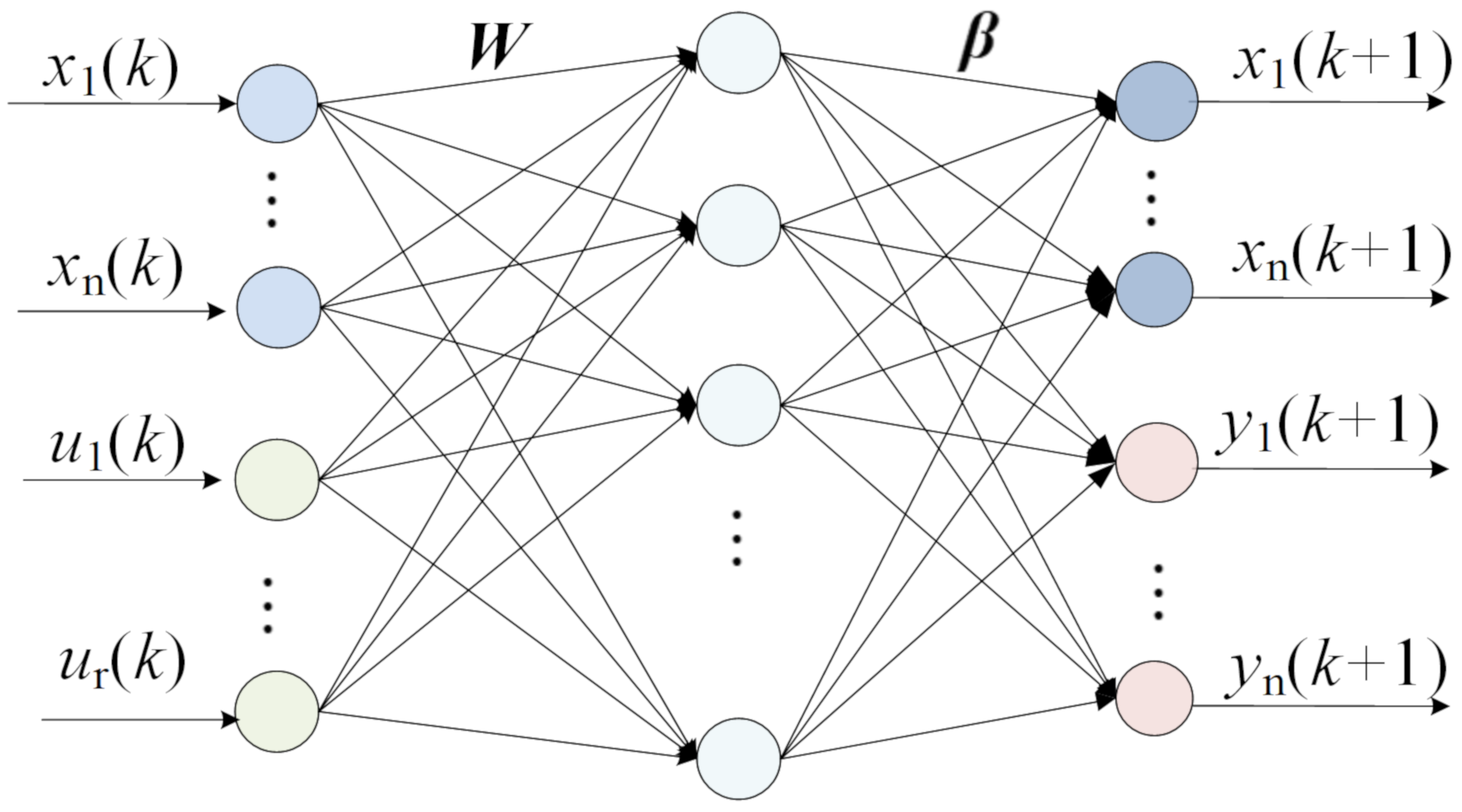
To obtain the linear state space model with AFOS-ELM, the data used to train the ELM are normalized as

$$\overline{x}=\frac{x-x_{\min }}{x_{\max }-x_{\min }}$$

(28)

The inverse-free ELM neural network described in Section 2 is used in the ELM initialization. The inputs of the AFOS-ELM are the input variables u(k) and the state variables x(k) of the state space model in Equation (25). The outputs of the ELM are the state variables x(k + 1) and the output variables y(k) of the SSM. Then, the construction of the AFOS-ELM is shown in Figure 1.

The OS-ELM adopts linear output nodes, and the analytical expression of network output can be described as

$${\mathit{y}}_{ELM}(k)={\displaystyle \mathit{\sum }_{i=1}^l{\mathit{\beta }}_i(k)f({\mathit{W}}_i{\mathit{x}}_{ELM}(k)+b_i)}$$

(29)

where ${\mathit{y}}_{ELM}(k)=\left[\begin{array}{cc}{x}^T\left(k+1\right)& y^T\left(k\right)\end{array}\right]$, ${\mathit{x}}_{ELM}(k)=\left[\begin{array}{cc}{x}^T\left(k\right)& u^T\left(k\right)\end{array}\right]$ are the neural network output vector and input vector.

The partial derivative of network output to network input is calculated by

$$\frac{\partial y_{ELM}(k)}{\partial x_{ELM}(k)}={\displaystyle \sum _{j=1}^l\frac{\partial y_{ELM}(k)}{\partial h_j(k)}\frac{\partial h_j(k)}{\partial x_{ELM}(k)}}={\displaystyle \sum _{j=1}^l{\beta }_j(k)}{W}_j\dot{f}(W_j{x}_{ELM}(k)+b_j)$$

(30)

$$\dot{f}(W_j{x}_{ELM}(k)+b_j)=\frac{e^{-W_j{x}_{ELM}(k)-b_j}}{{(1+e^{-W_j{x}_{ELM}(k)-b_j})}^2}$$

(31)

Therefore, the parameters in Equation (27) can be calculated according to Equations (30) and (31), and then the SSM in Equation (26) is obtained at time k.

5. Simulation and Discussion

5.1. Data Process

In order to verify the method of establishing SSM online based on the neural network proposed in this paper, the test data of a twin spool hybrid exhaust afterburner turbofan aero-engine are used for modeling and validation. The research is carried out in the environment of Win11, Intel(R) CORE(R) i5-12600Kf CPU, and 32G RAM.

Since the data come from the engine test, the measurement noise is inevitable. To avoid the impact of outliers on modeling accuracy, the local singularity estimation capability of wavelets and the residuals of the signal wavelet transform can be used to determine the residual threshold for outlier discrimination [35,36].

The residual of the original signal S after L-layer wavelet decomposition can be described by

$$R_e=S-S_{\mathrm{S}}$$

(32)

where S_S are the low-frequency reconstructed signal after L-layer decomposition.

When the residual is small, the low-frequency reconstructed signal approaches the original signal. When the residual is large, there is a relatively large-amplitude high-frequency noise superimposed on the measured signal, which can be seen as an outlier. Taking the fuel data of an engine test as an example, the “db8” wavelet with scale 7 is used to detect the outliers. A total number of 111,406 data are collected in this test, and the residual distribution of fuel flow W_f is shown in

Table 1. Statistics of wavelet transform residual distribution of W_f.

	Residual Distribution
Residual interval/%	[−∞, −7.04]	[−7.04, −4.94]	[−4.94, −2.83]	[−2.83, −0.721]	[−0.721, 1.39]	[1.39, 3.49]	[3.49, 5.6]	[5.6, 7.71]	[7.71, 9.82]	[9.82, ∞]
Number of data	9	7	16	1348	109,786	207	17	8	2	6

.

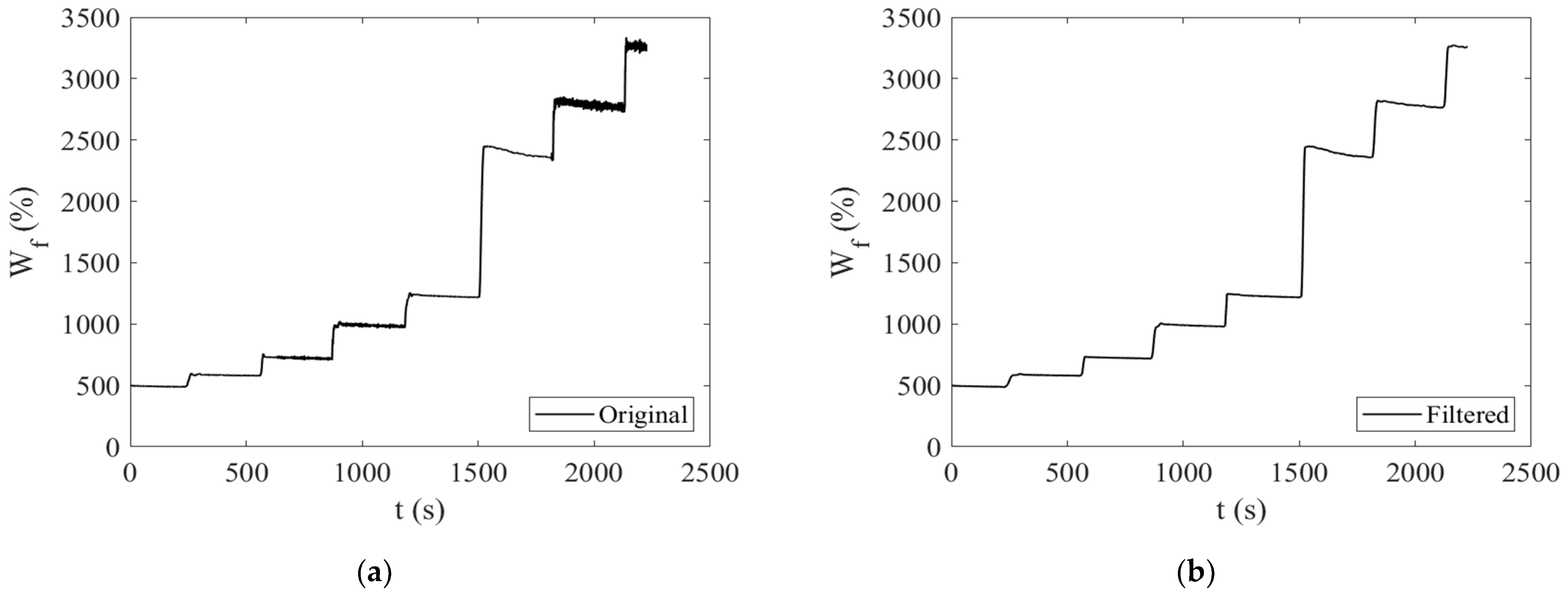
It can be seen from Table 1 that the data in the range of residual [−0.721%, 1.39%] account for 98.54% of the total data, and the data in the range of residual [−2.83%, 3.49%] account for 99.94% of the total data. The data distribution in the range of residual greater than 3.49% or less than −2.83% does not tend to decrease with the increase of residual. Therefore, the threshold for outlier identification is set to −2.83% and 3.49%. The data with residuals beyond this range are considered outliers, which are replaced by the average value of the data before and after them. For continuous outliers, they are replaced by linear interpolation of the reasonable data before and after them. After replacing the outlier data, the “db8” wavelet with scale 7 is adopted to filter the signal. Taking fuel data as an example, the comparison of data before and after filtering is shown in Figure 2a,b.

It can be seen from Figure 2 that the noise in the filtered data is significantly suppressed, which is helpful to establish the SSM in a data-driven way. Then, the data are normalized with Equation (27).

5.2. AFOS-ELM Validation

The input vector for a twin spool turbo-fan engine control system is $u(k)={[W_f(k),A_8(k)]}^T$, and A₈ is the nozzle throat area. The measured output vector besides rotor speeds is $y(k)={[P_3(k),T_6(k),P_6(k),F(k)]}^T$, where P₃ is the total pressure at compressor outlet, T₆, P₆ are the total temperature and total pressure at low-pressure turbine outlet, and F is the thrust. The state vector is $x(k)={[n_1(k),n_2(k)]}^T$; n₁ and n₂ are the low-pressure rotor speed and the high-pressure rotor speed.

According to the construction of AFOS-ELM in Figure 1, the input vector of the ELM is ${\mathit{x}}_{ELM}(k)={\left[\begin{array}{cccc}{W}_f(k)& A_8(k)& n_1(k)& n_2(k)\end{array}\right]}^T$. The output vector of the ELM is ${\mathit{y}}_{ELM}(k)={[n_1(k+1), n_2(k+1), P_3(k), T_6(k), P_6(k), F(k)]}^T$.

The first 30% of the engine test data sequence are adopted to initialize the ELM based on the inverse-free ELM offline. When the root mean square error is less than 6.5% or the number of hidden layer nodes increases to more than 100, the offline training stops. The number of hidden layer nodes is automatically set to 86 in this research.

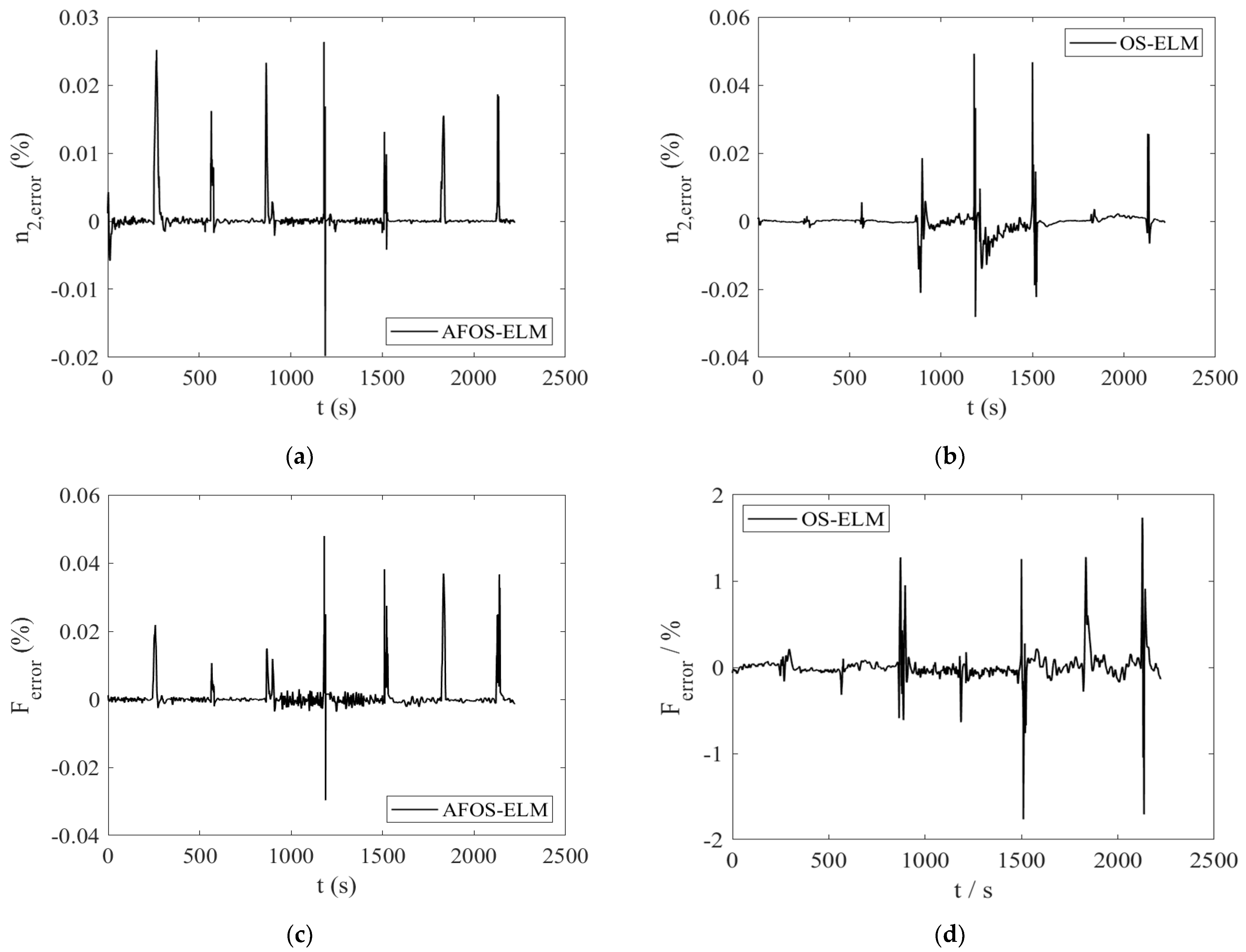
The AFOS-ELM is used to update the output weights online for all the engine test data. The n₂ output of the AFOS-ELM is compared with the engine test data in Figure 3. The relative output errors of n₂ and F are compared with that of the traditional OS-ELM without the forgetting factor in Figure 4. The detail errors of the ELM outputs are listed in

Table 2. Relative error of neural network output (%).

Method	Error Type	Variables
		n1(k + 1)	n2(k + 1)	P3(k)	T6(k)	P3(k)	F(k)
AFOS-ELM	Average error	0.0013	0.0008	0.0016	0.002	0.0014	0.0013
	Maximum error	0.0649	0.0263	0.2084	0.2747	0.0866	0.0479
	Standard deviation	0.0043	0.0026	0.0055	0.0051	0.004	0.0037
OS-ELM	Average error	0.0019	0.0014	0.3218	0.5854	0.2815	0.0831
	Maximum error	0.1419	0.0492	5.8795	16.52	6.8424	1.7649
	Standard deviation	0.0042	0.0028	0.4385	1.0432	0.5142	0.1572

.

From Figure 3 we can see that both the AFOS-ELM and OS-ELM output n₂(k + 1) track the engine test data well in the acceleration process. From Figure 4 we can see that the relative errors of n₂(k + 1) and F(k) are both smaller than 0.05% with the AFOS-ELM method, which is much smaller than that of the OS-ELM method, and the adaptive forgetting factor enhances the modeling accuracy both at the dynamic state and at the steady state.

It can be seen from Table 2 that the errors of two rotor speeds are very small for both AFOS-ELM and OS-ELM, the maximum error occurs at n₁ with OS-ELM method, which is 0.1419%, and the average error is less than 0.002%, which is much better than that of the component-level model [37]. For the other output variables, the AFOS-ELM method shows greater advantage than the OS-ELM method. The maximum error of AFOS-ELM occurs at T₆, which is 0.2747%, and the max average error occurs also occurs at T₆, which is 0.002%, while for OS-ELM, the maximum error and the max average error also occur at T₆, which are 16.52% and 0.5854%, respectively, and the figures are much bigger than that of the AFOS-ELM. AFOS-ELM can model the state space configuration nonlinear model well. It can process the engine failure data and ensure the accuracy of the current output. The adaptive forgetting factor can also deal with the rapid change caused by the large dynamic and maintain a high accuracy.

5.3. State Space Model Validation

Based on the analytical expression of the AFOS-ELM model established above, the SSM can be derived by partial derivative calculation. Taking the calculation of parameter $a_{11}(k)$ as an example, according to Equations (3) and (27), we have

$$a_{11}(k)=\frac{\partial n_1(k+1)}{\partial n_1(k)}=\frac{\partial n_1(k+1)}{\partial \mathit{H}(k)}\frac{\partial \mathit{H}(k)}{\partial n_1(k)}={\displaystyle \sum _{j=1}^l{\beta }_{1j}}{W}_{1j}\dot{f}(W_{1j}{n}_1(k)+b_j)$$

(33)

Applying the calculation process of $a_{11}$ o the other parameters of the SSM, the calculation of all state space matrix parameters at time k can be achieved, and the SSM at time k is established.

In order to validate the effectiveness of the SSM established in this paper, the models established at different times are selected to demonstrate their output prediction ability over future time, which is essential for model-predictive control and performance-seeking control of aero-engines.

The prediction output of SSM at future time can be obtained through the response calculation of a discrete-time system.

$$\begin{array}{cc}\hfill x(k+1)& =\mathit{A}(k)x(k)+\mathit{B}(k)u(k)\hfill \\ \hfill x(k+2)& =\mathit{A}(k)x(k+1)+\mathit{B}(k)u(k+1)\hfill \\ & ={\mathit{A}}^2(k)x(k)+\mathit{A}(k)\mathit{B}(k)u(k)+\mathit{B}(k)u(k+1)\hfill \\ & \cdots \cdots \\ \hfill x(k+p)& ={\mathit{A}}^p(k)x(k)+{\displaystyle \sum _{i=k}^{k+p-1}{\mathit{A}}^{k+p-1-i}}(k)\mathit{B}(k)u(i)\hfill \\ \hfill y(k+p)& =\mathit{C}(k){\mathit{A}}^p(k)x(k)+{\displaystyle \sum _{i=k}^{k+p-1}\mathit{C}(k){\mathit{A}}^{k+p-1-i}}(k)\mathit{B}(k)u(i)+\mathit{D}(k)u(k+p)\hfill \end{array}$$

(34)

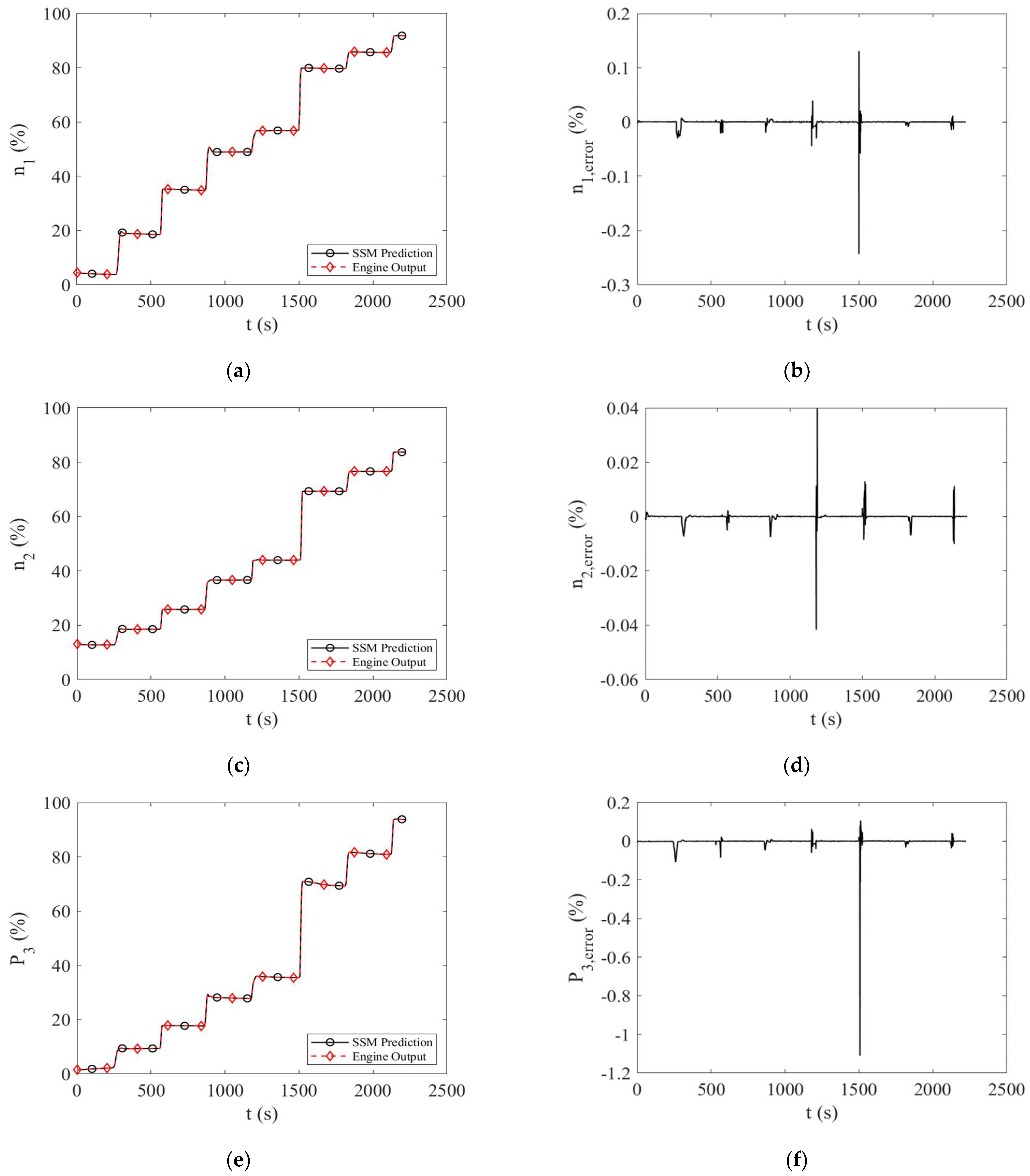
Taking p = 5 as an example, the error between the SSM prediction output and the engine output is compared. The results of prediction are shown in Figure 5a–l, where the “SSM Prediction” represents the prediction output of the SSM proposed in this paper, and “Engine Output” represents the engine test data at k + p.

As can be seen from Figure 5, the maximum prediction error at time k + 5 occurs at $P_3$ around 1500 s, where a sudden acceleration occurs and the thrust F increases about 40.6%. Except for F, the other variables all reach their biggest prediction error at this moment. Under such a big dynamic, the max prediction error occurred at $P_3$ and is about 1.1%. The max prediction error of the low-pressure rotor speed is less than 0.3% when the low-pressure rotor speed n₁ increases about 22.9%, while the error is more than 0.4% in the component-level-model-based online state space modeling method in reference [21] for time k + 5 output prediction when the low-pressure rotor speed decreases by about 12% (there is no other common variable that can be compared in reference [21]). The prediction accuracy of the SSM established by the method described in this paper shows great advantage, and it can predict the varying of the engine test data well.

In order to validate the real-time performance of the SSM proposed in this paper, the time consumption of the AFOS-ELM online modeling process and the SSM modeling process are evaluated. The simulation platform is as described above; the modeling process is carried out three times. The neural network is established online based on 111,406 groups of engine test data, and 111,405 SSMs are obtained from the first data to the last-1 data, and the average time for modeling the 111,405 SSMs based on AFOS-ELM is 183.958 s. The online network weights updating and online SSM calculation process of each step takes an average of 1.7 ms. It is lower than the sampling step of the aero-engine, which is about 20 ms. Therefore, this modeling method can meet the real-time requirements of the aero-engine.

6. Conclusions

An online data-driven state space modeling method based on AFOS-ELM is proposed in this paper, which provides a mechanism-model-free state space modeling method for a complex nonlinear system. The inputs and outputs of the AFOS-ELM are determined according to the description of the SSM. The partial derivative calculation based on the analytical model of the AFOS-ELM provides an alternative for deference-based calculation in the Jacobian matrix (state space matrix) calculation of SSM. The OS-ELM with adaptive forgetting factor shows great system dynamic capture ability and achieves high modeling accuracy at both steady state and dynamic state on the engine test dataset, which means the SSMs obtained from it have the ability to predict the system output in future time accurately.

The inverse free-ELM algorithm used in the OS-ELM initialization can automatically determine the most appropriate number of the hidden layer nodes, which reduces the trail time and enhances the modeling efficiency.

The SSM is established online at each sampling time of the engine operation and has high real-time property, which gives it the potential to be further used in model-based control and health management research.