
Mitigation of Low-Frequency Oscillation in Power Systems through Optimal Design of Power System Stabilizer Employing ALO

 ,
,  ,
,  ,
,  and
and 
Abstract
1. Introduction
1.1. Motivation and Incitement of the Paper
1.2. Literature Review
1.3. Research Gaps
1.4. Contribution of the Manuscript
- In this manuscript, the application of the dual-input PSS with optimally tuned controller parameters uses the most recent ALO technique.
- As presented in the results section, all of the simulation results are superior to the other applied techniques.
- In addition, the authors tried to compare the results of the dual-input PSS with the single-input PSS, base case and classical system.
- Further, a practical utility network was utilized, which is from a developing nation Ethiopia. As in the developing nations, such as Ethiopia, practical systems are facing challenges from the low-frequency oscillations. Further, the system network is going to be upgraded, which makes the LFO problem more complex. Therefore, this work is very helpful for providing the solution to the utility network.
1.5. Organization of the Manuscript
2. Methodology
2.1. Power System Stabilizer
Types of Power System Stabilizers
2.2. Sizing of Power System Stabilizer Parameters
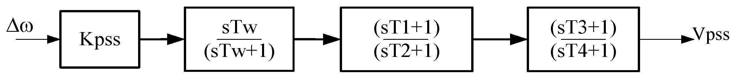
2.3. Modeling of Power System Stabilizer
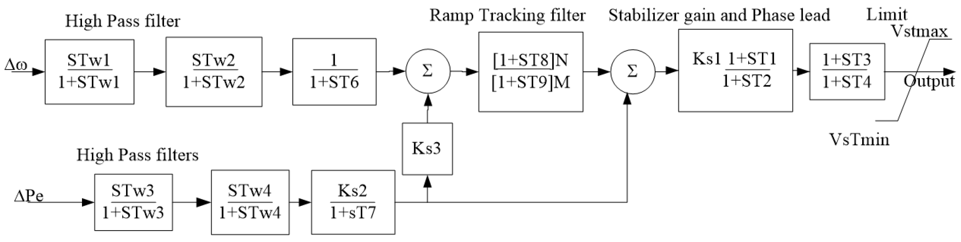
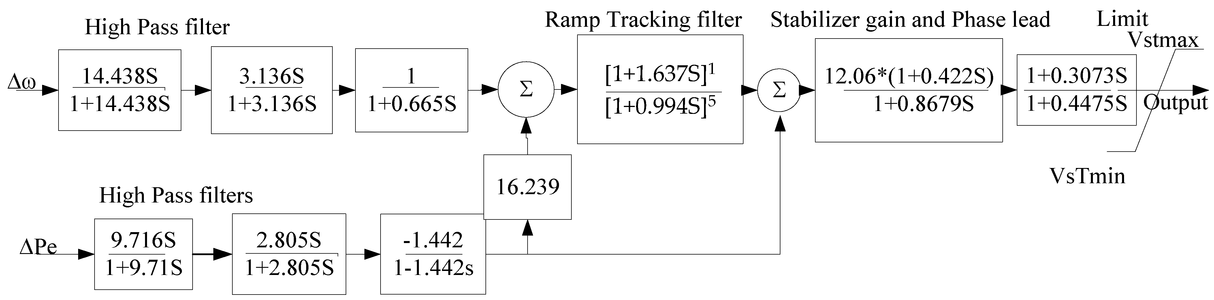
2.4. Dual-Input Power System Stabilizer
2.5. Problem Formulation
2.5.1. Objective Function
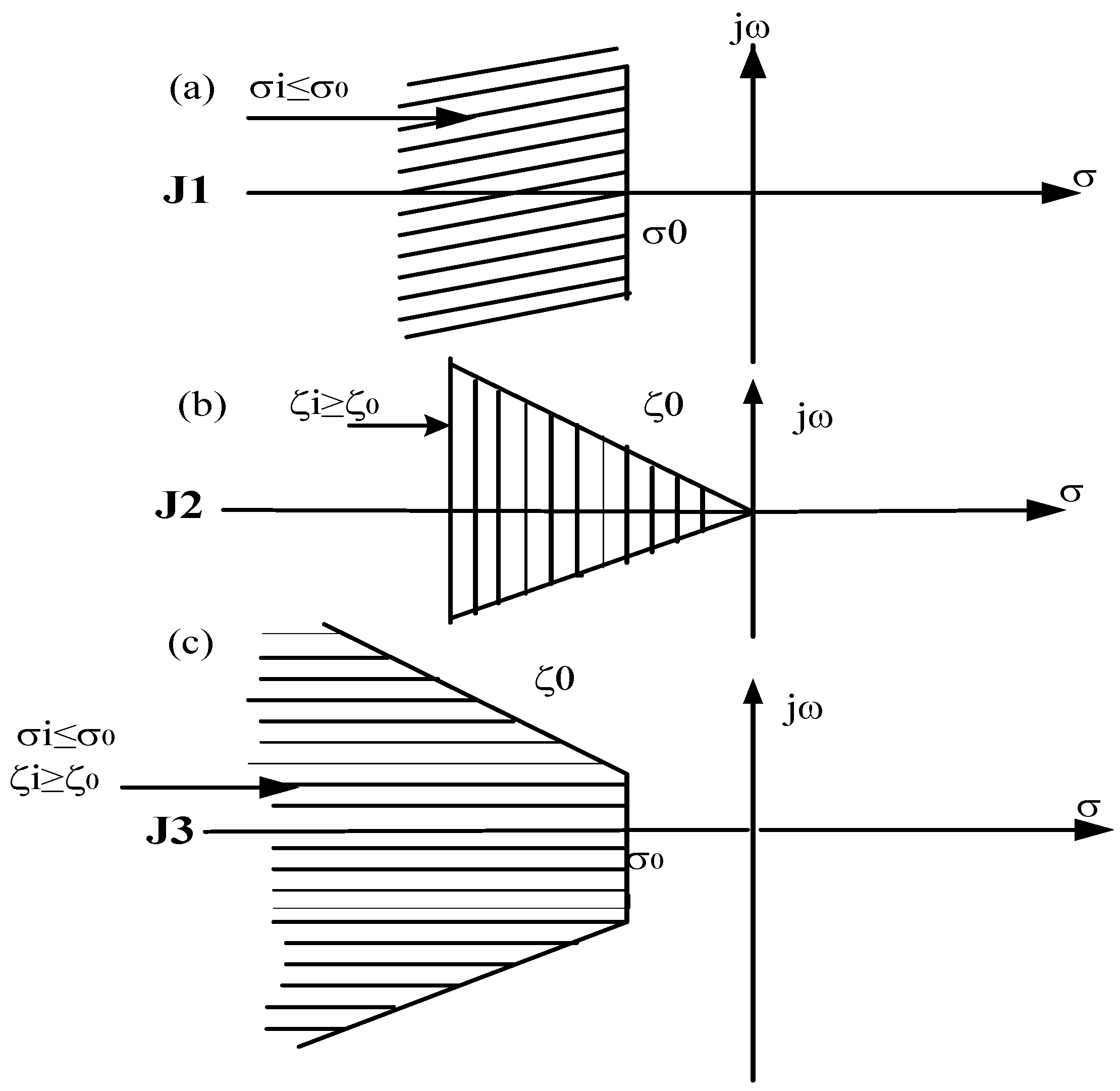
2.5.2. Constraint Equations
3. Ant Lion Optimization Problem
3.1. Operators of ALO Algorithm
3.2. Random Walk of Ants
3.3. Trapping in Ant Lion’s Pit
3.4. Sliding Ants towards Ant Lion
3.5. Catching Prey and Rebuilding Pit
3.6. Elitism
| Algorithm 1. The pseudo-codes of the ALO algorithm |
| Initialize the first population of ants and antlions randomly Calculate the fitness of ants and antlions Find the best antlions and assume it as the elite (determined optimum) While the end criterion is not satisfied for every ant Select an antlion using Roulette wheel Update c and d using equations above Create a random walk and normalize it given by the above equations in the random walk Update the position of ant using Equation (22) end for Calculate the fitness of all ants Replace an antlion with its corresponding ant it if becomes fitter Update elite if an antlion becomes fitter than the elite end while Return elite |
3.7. Optimal Sizing of Single-Input PSS
3.8. Optimal Parameter Sizing of Dual-Input PSS
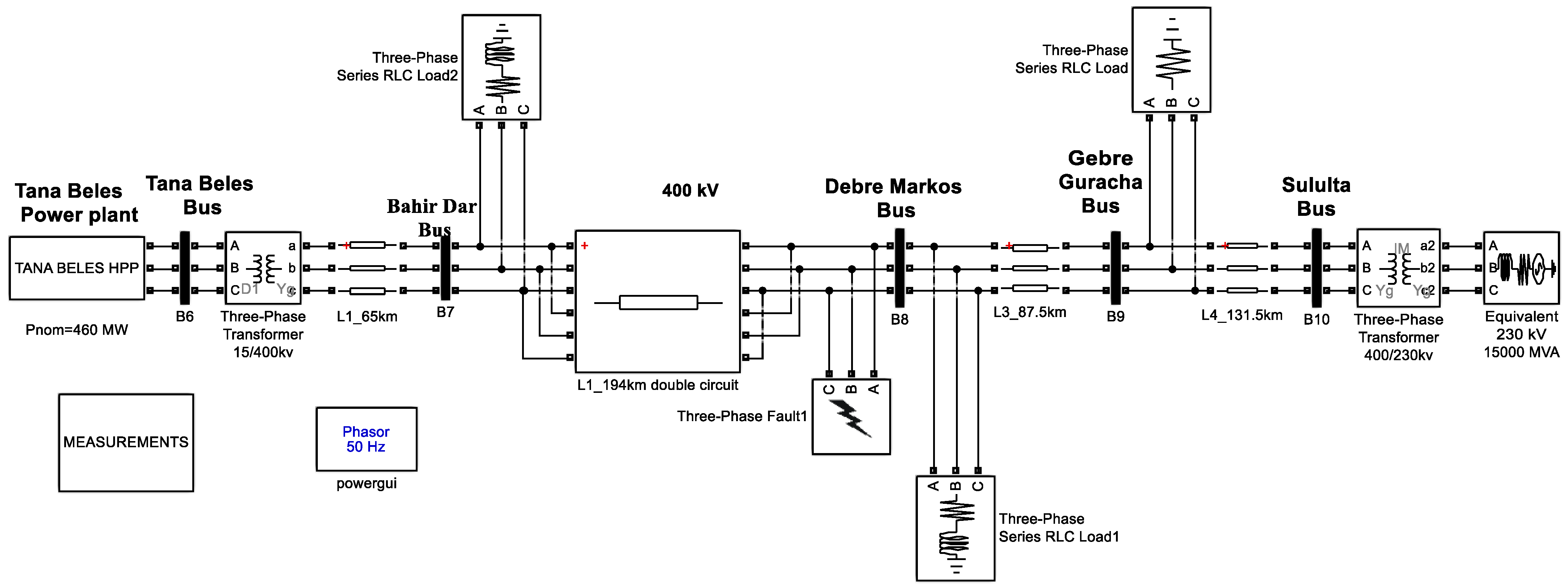
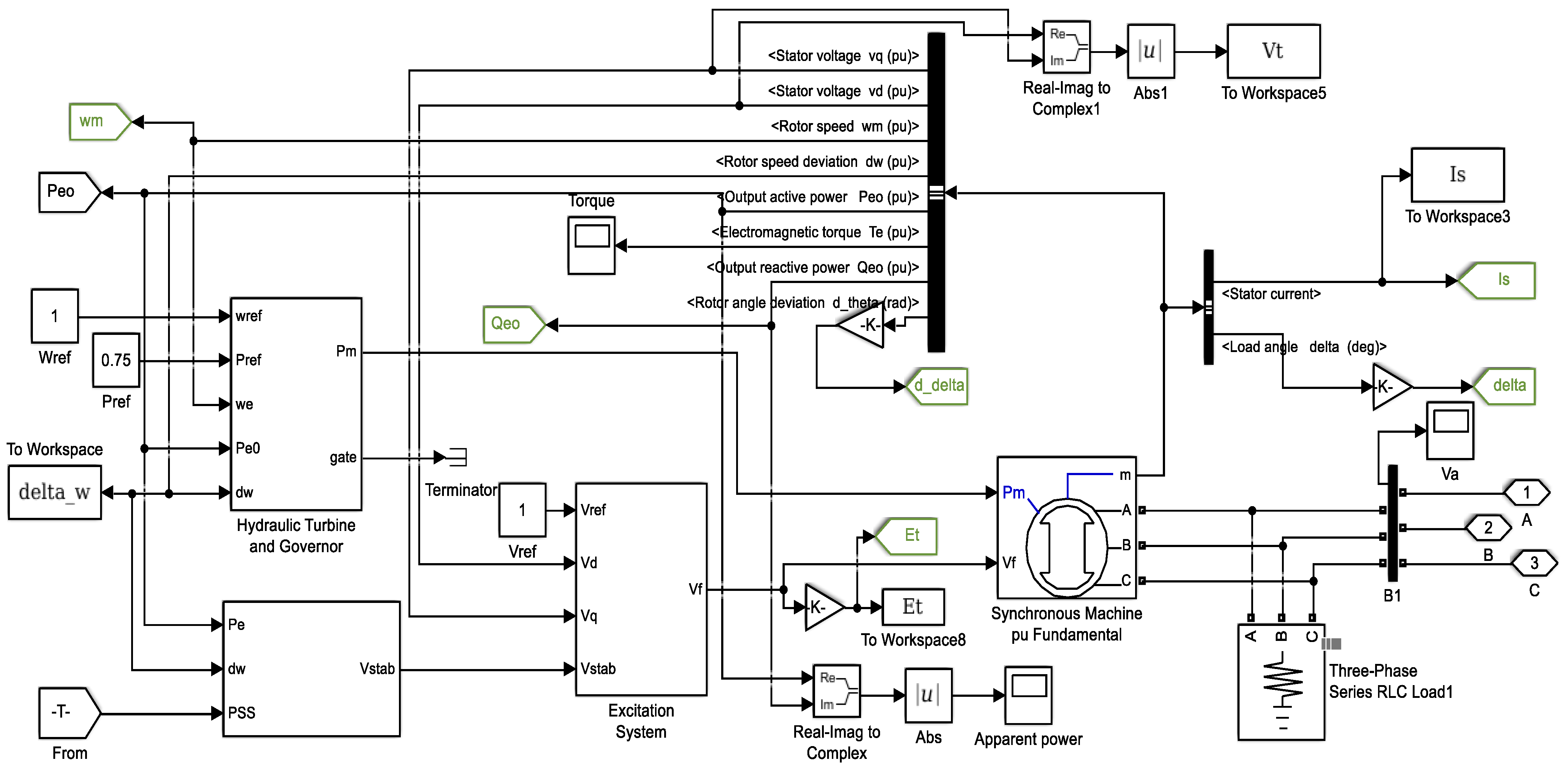
3.9. Overall System Diagram with MATLAB Simulink
4. Result and Discussion
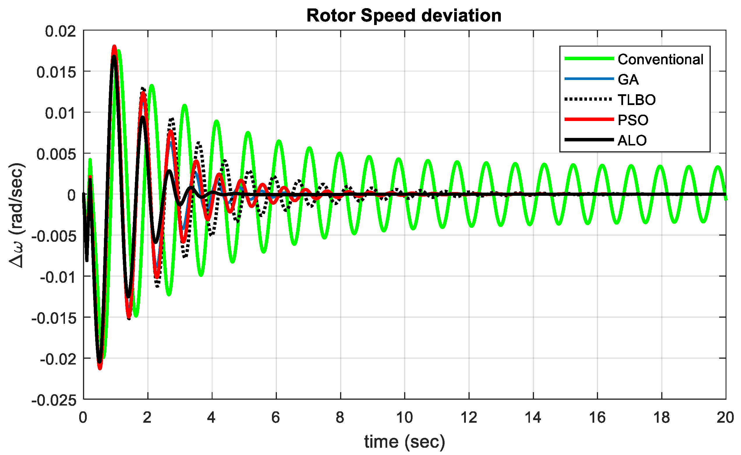
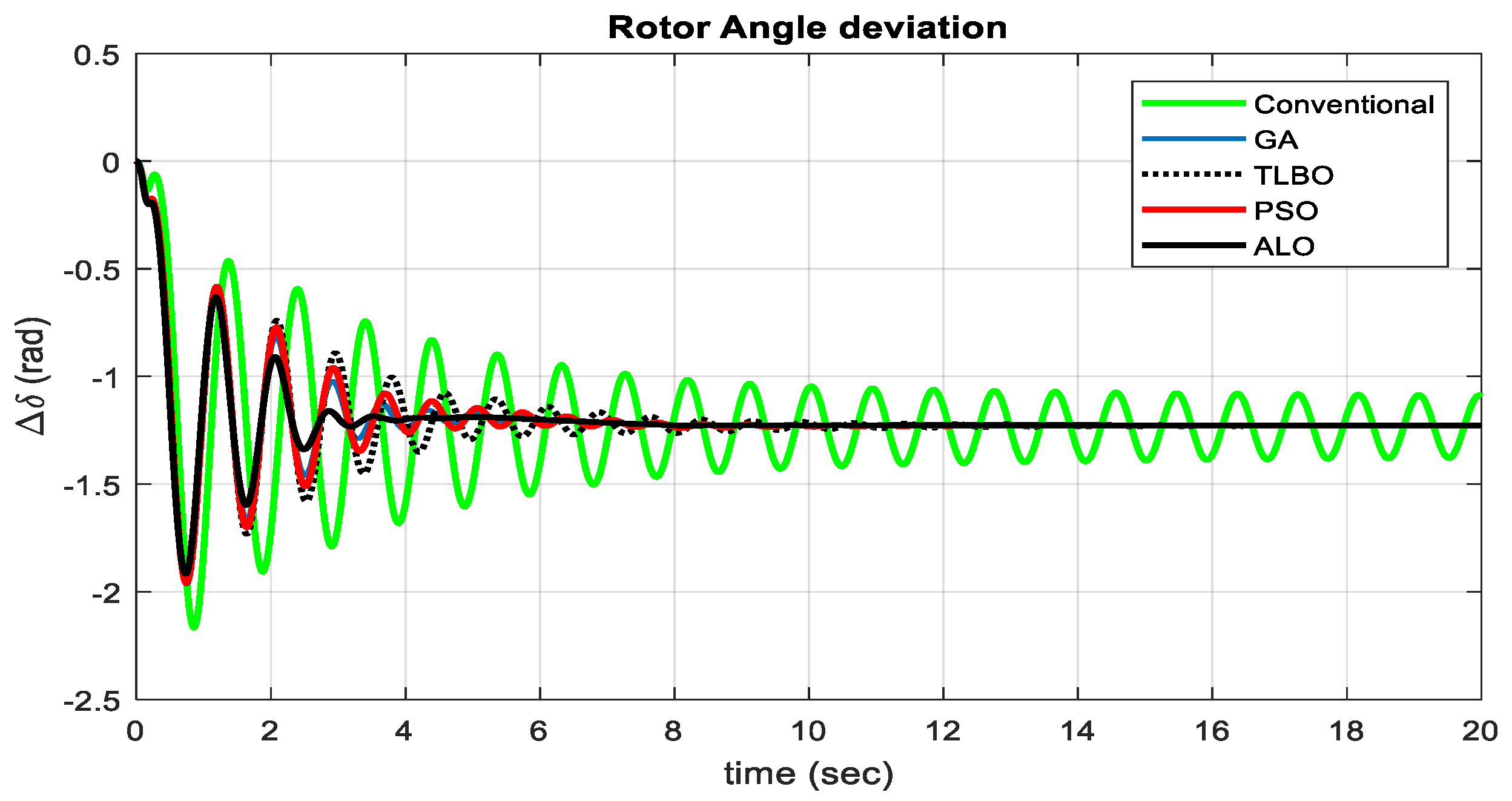
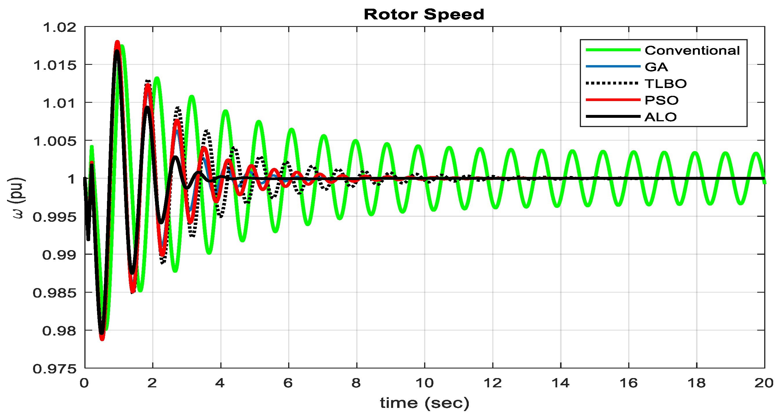
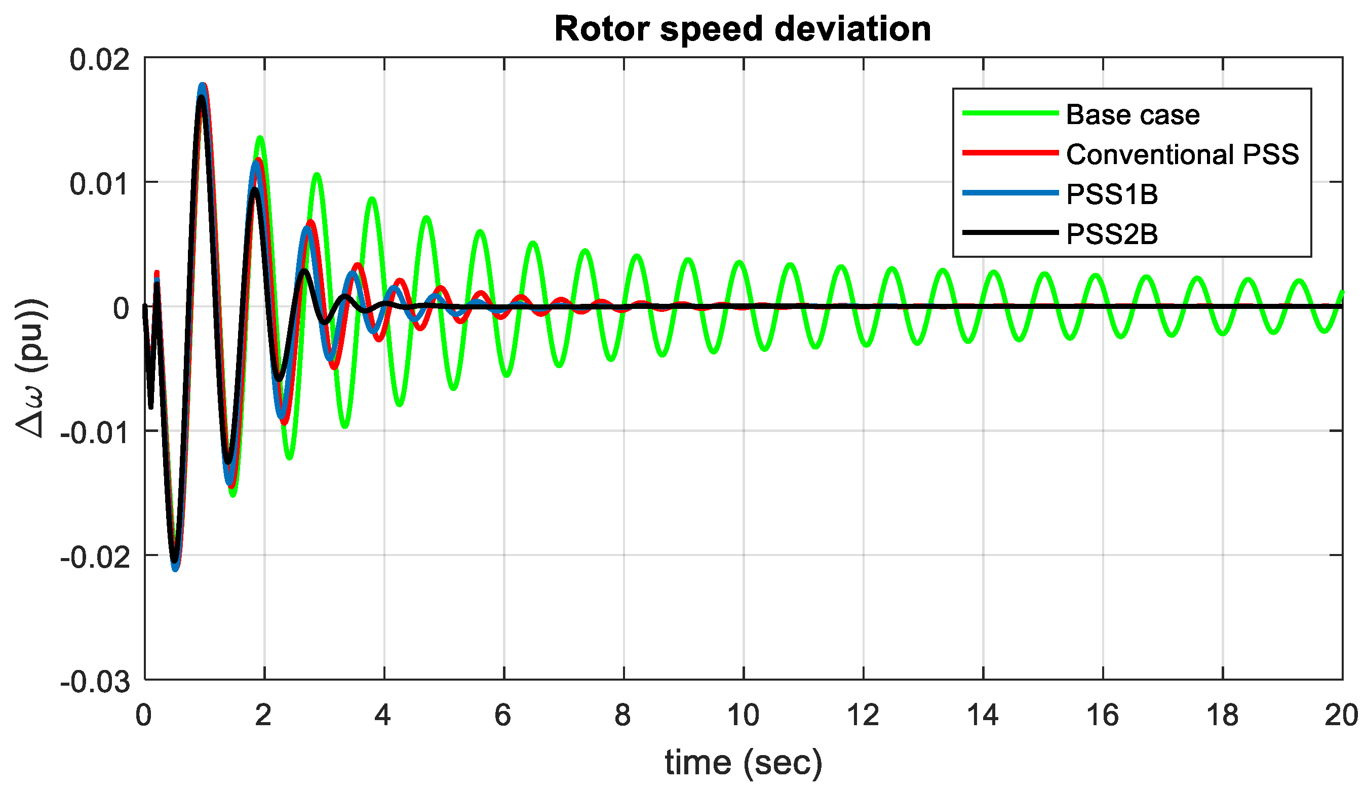
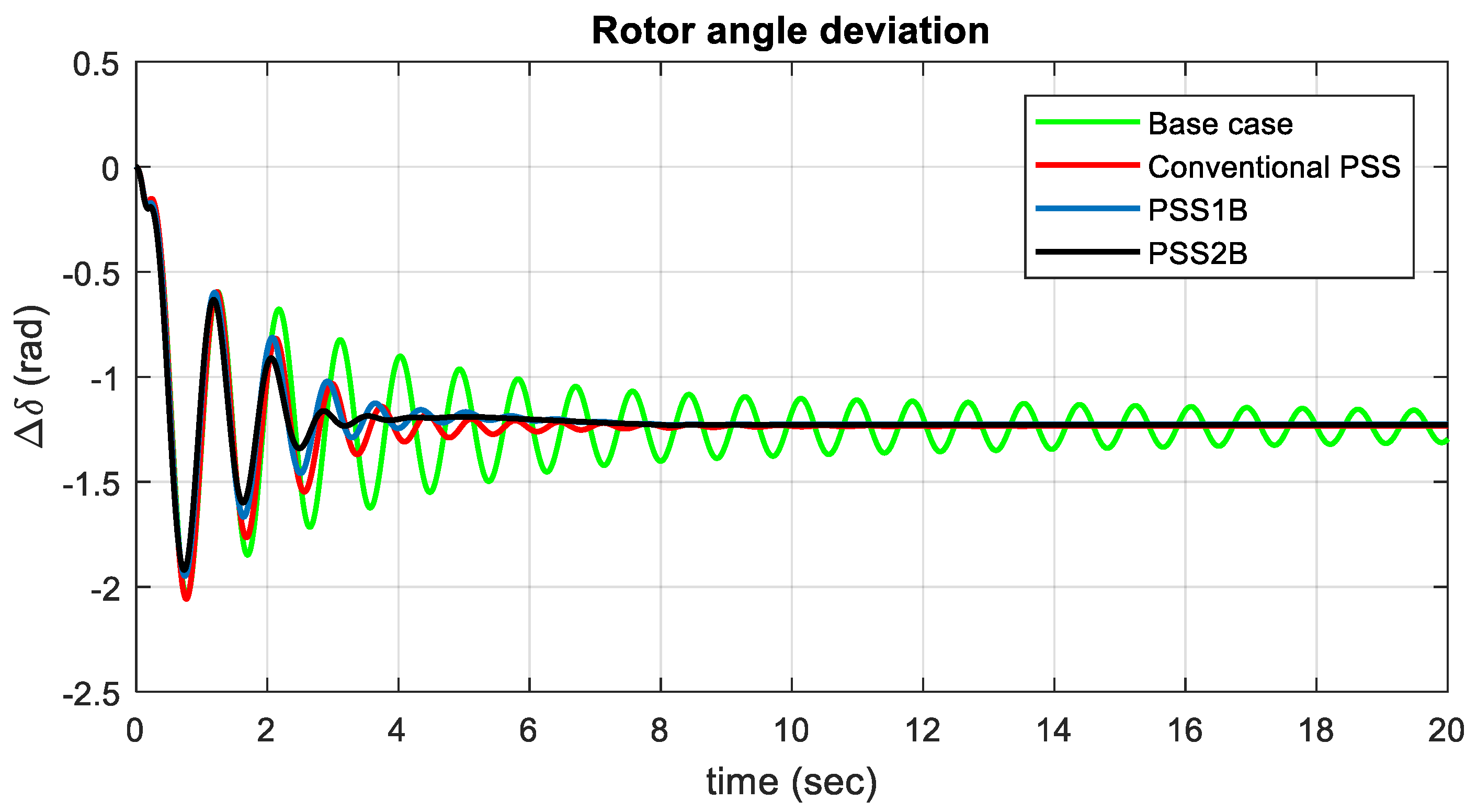
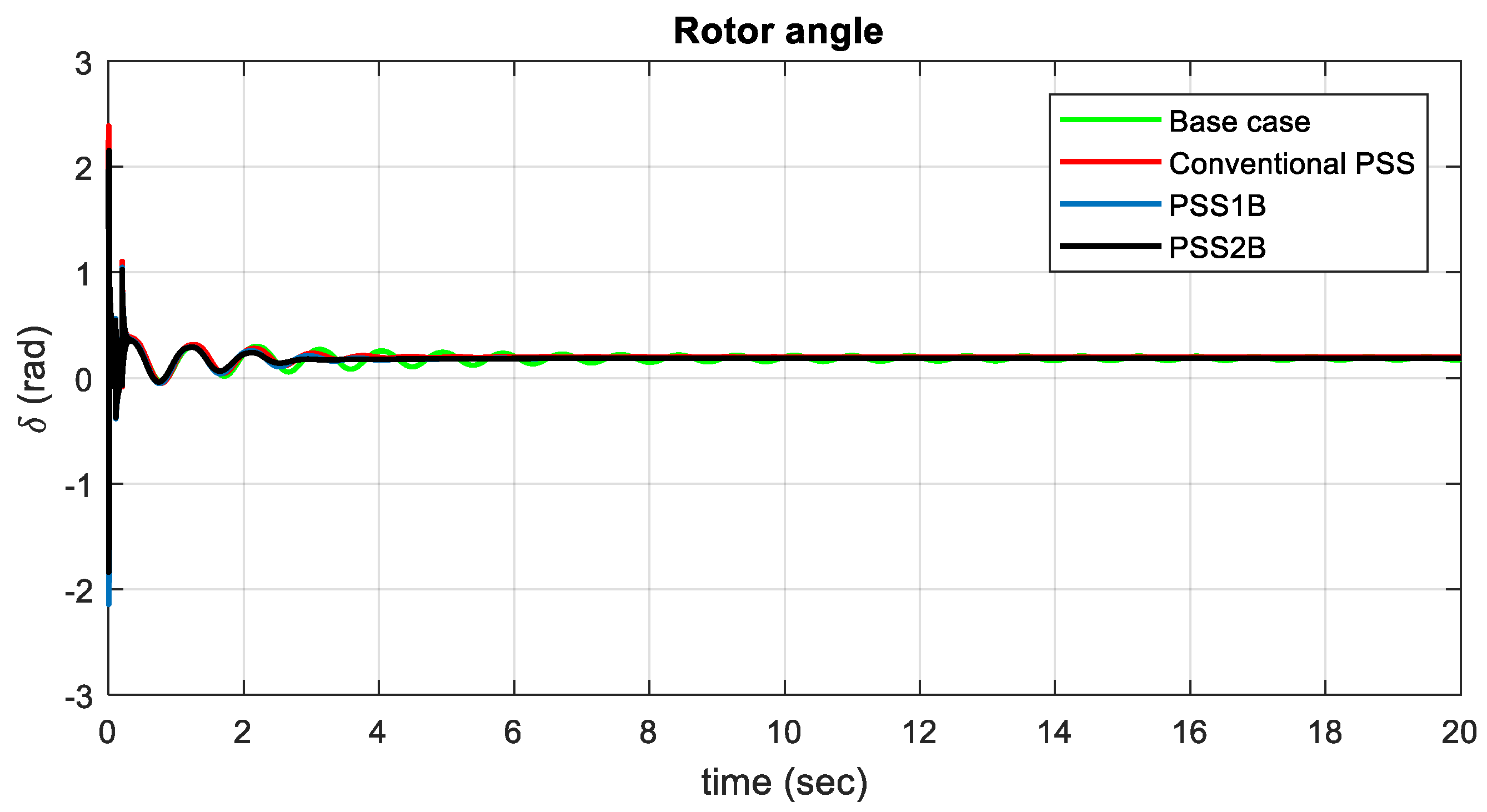
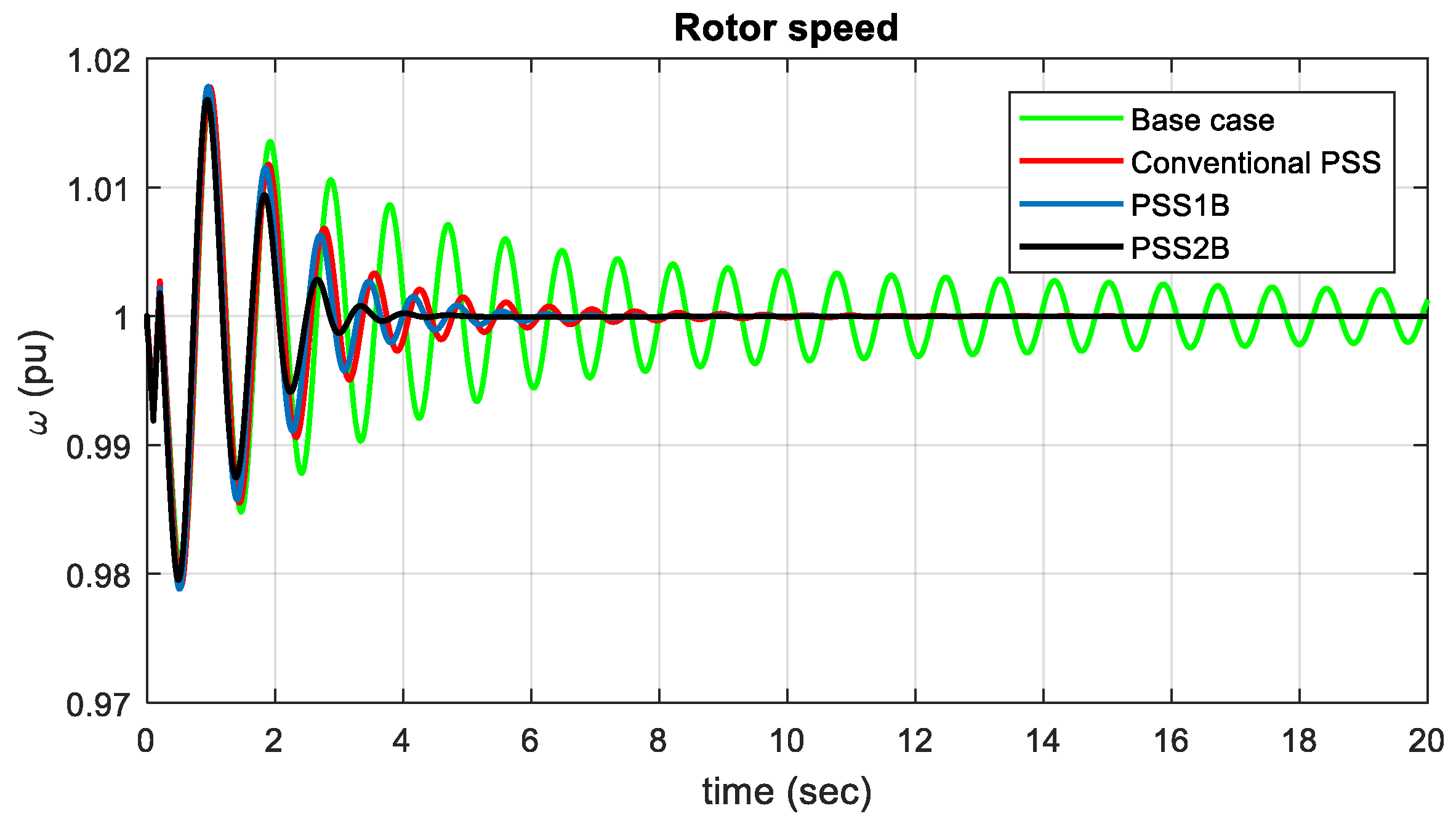
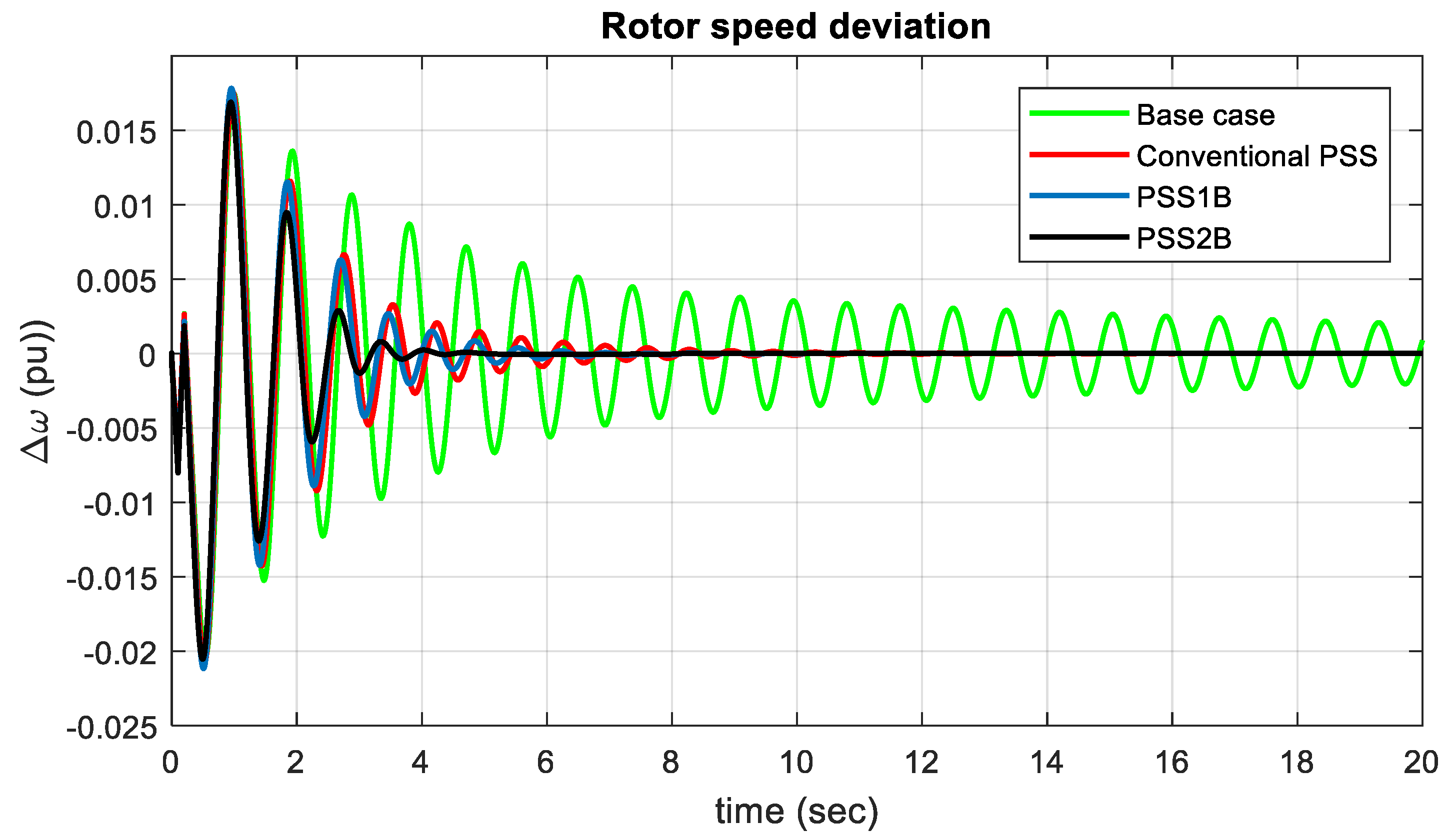
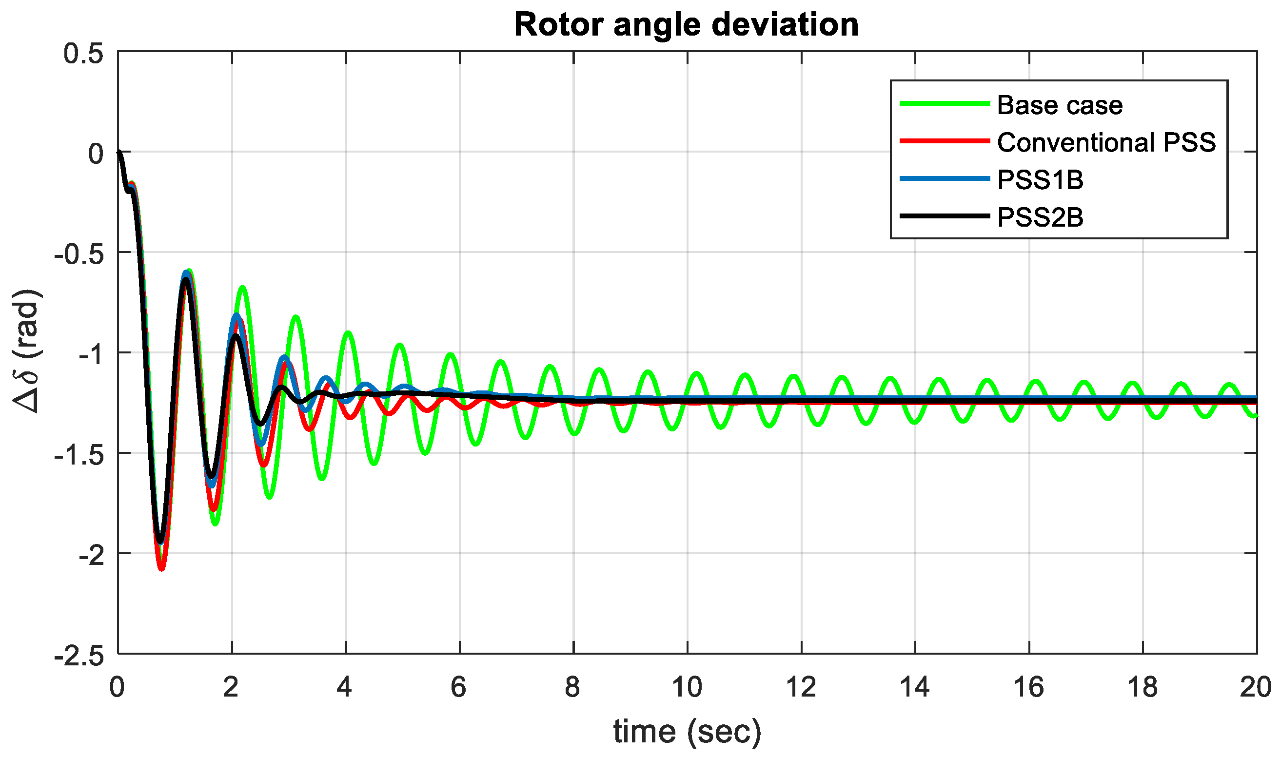
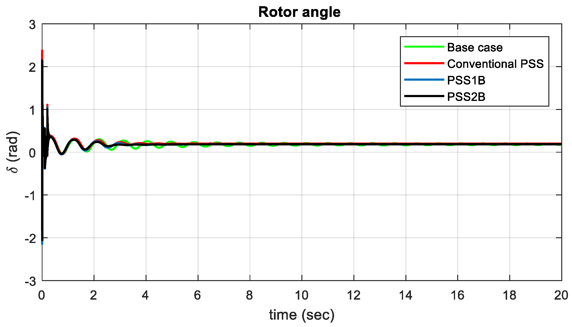
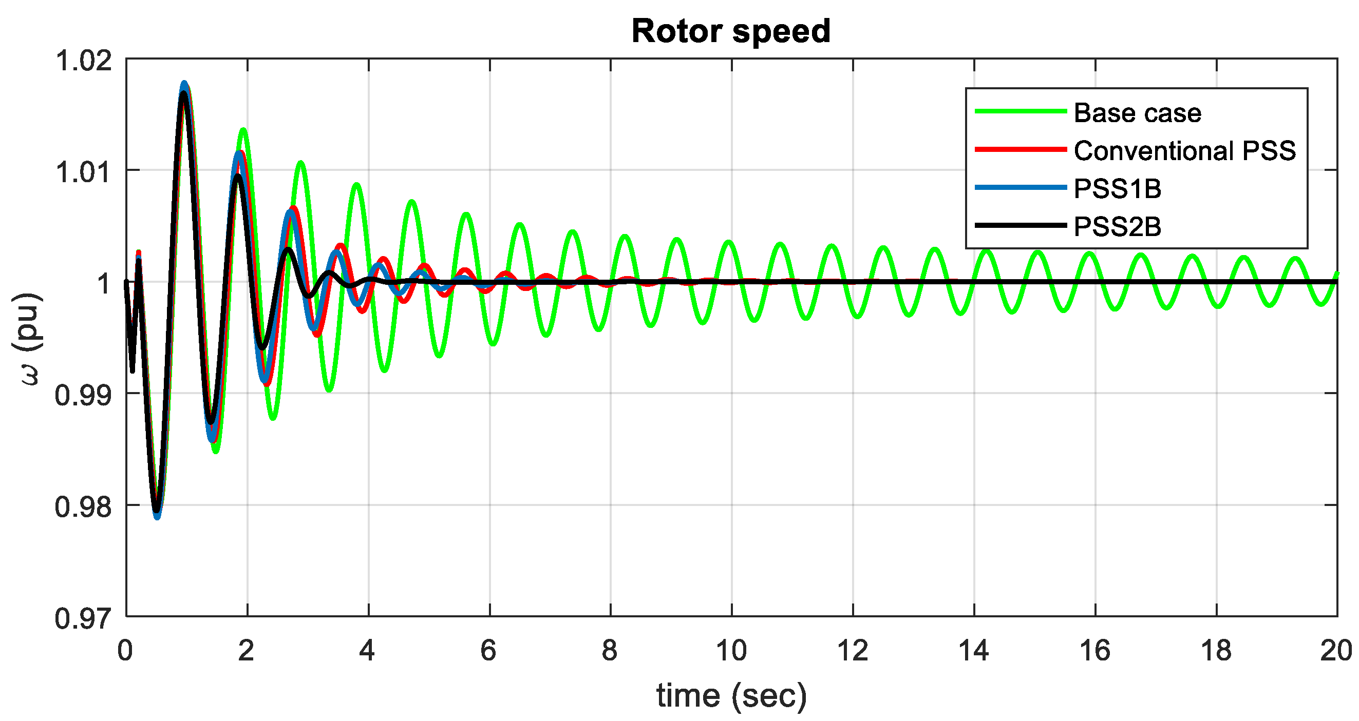
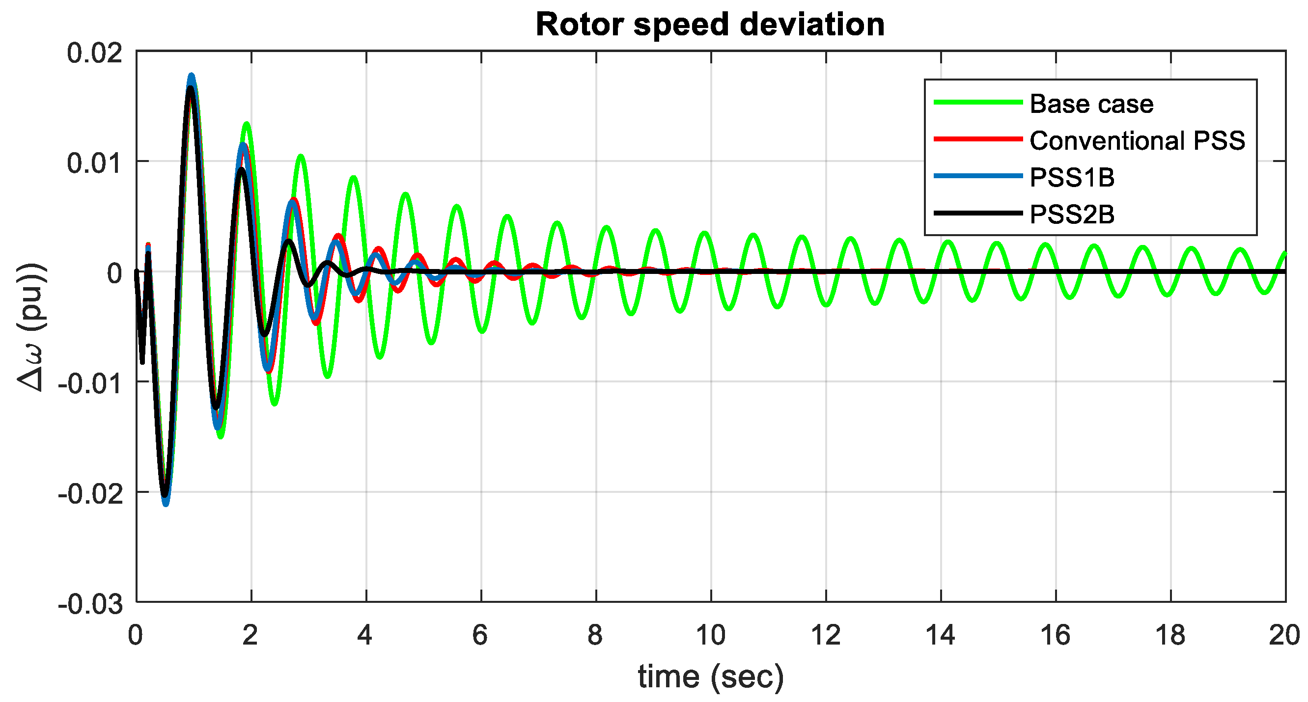
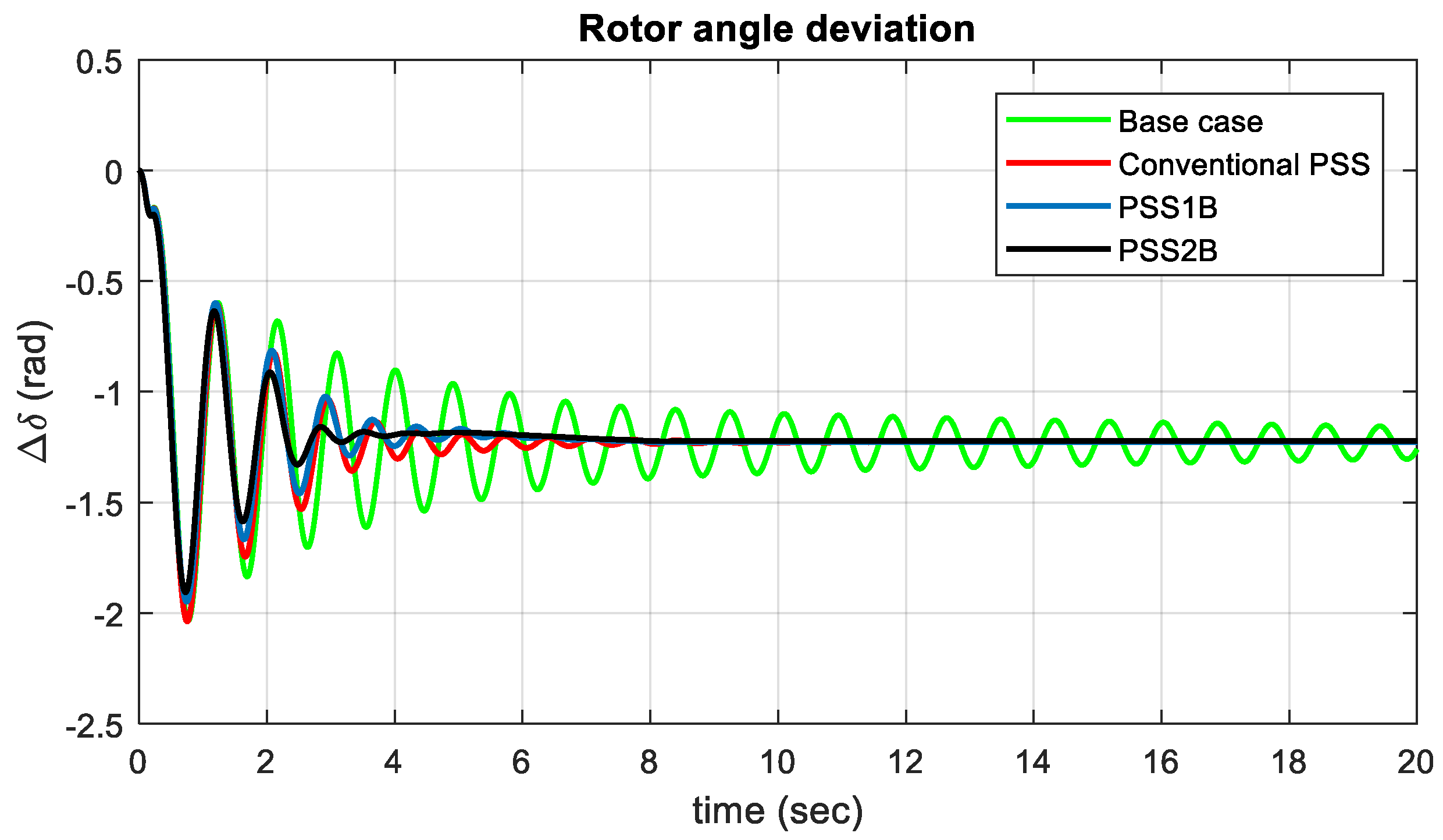
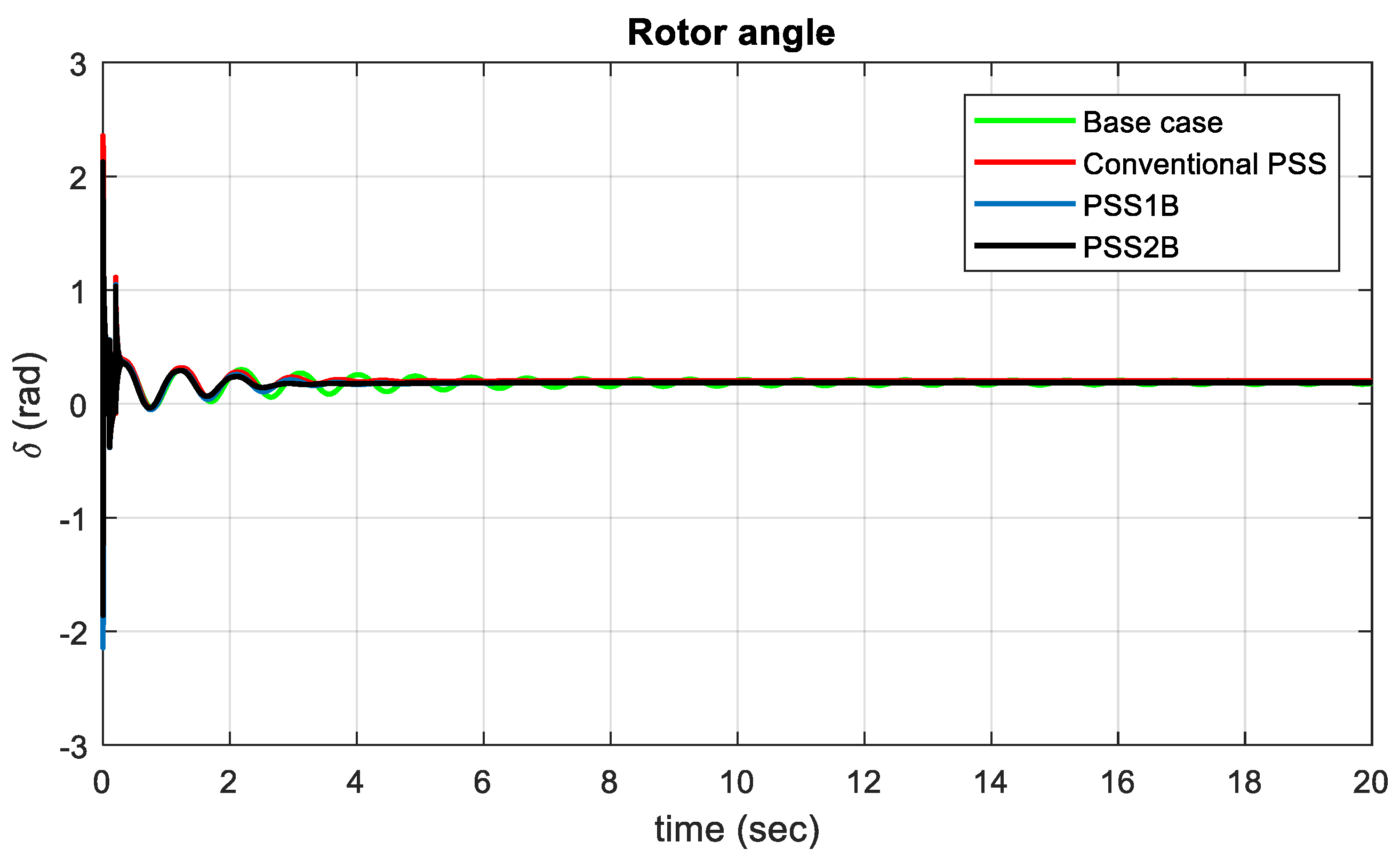
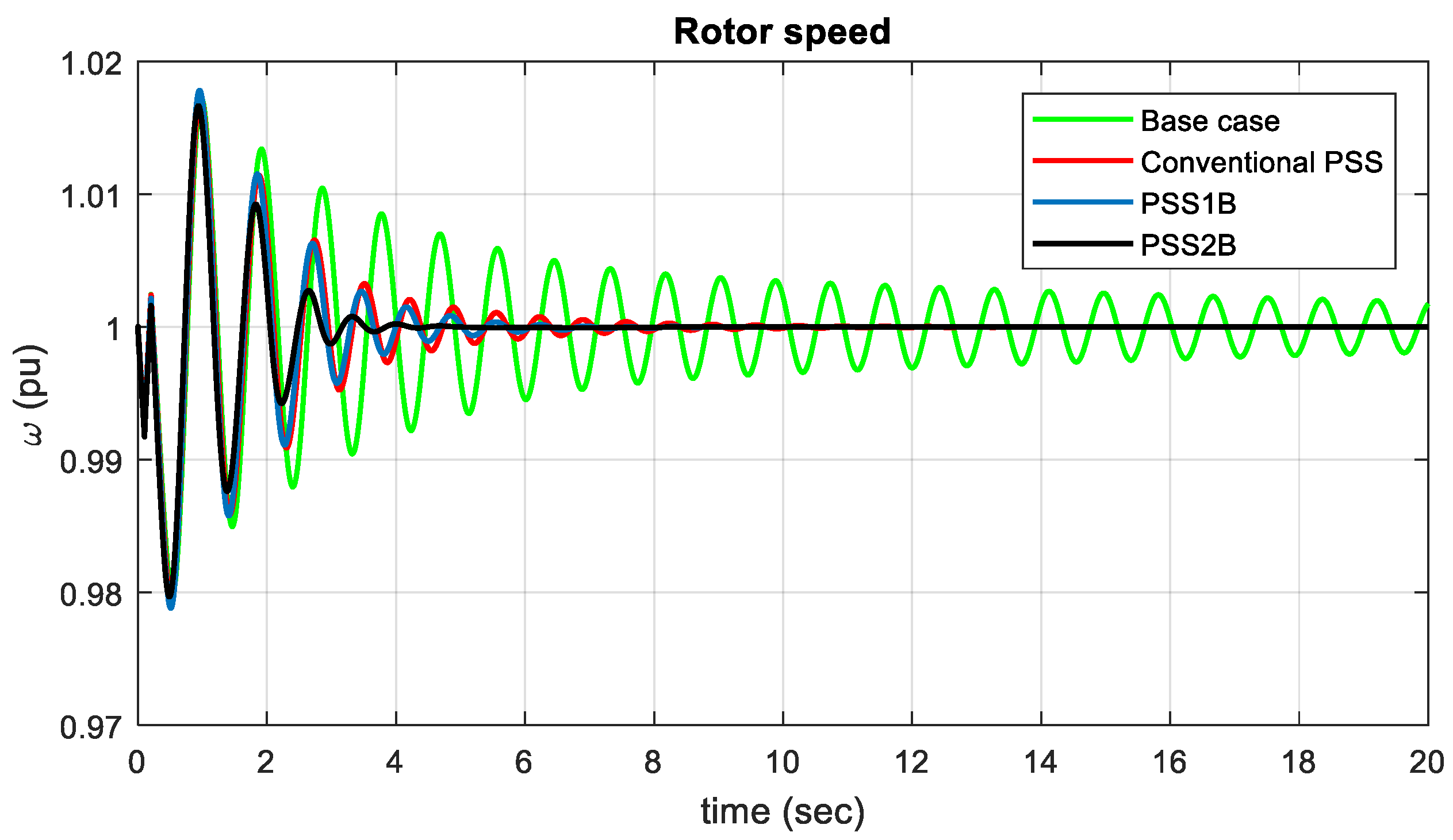
4.1. Time Domain Simulation Analysis
Eigenvalue Analysis and Minimum Damping Ratio
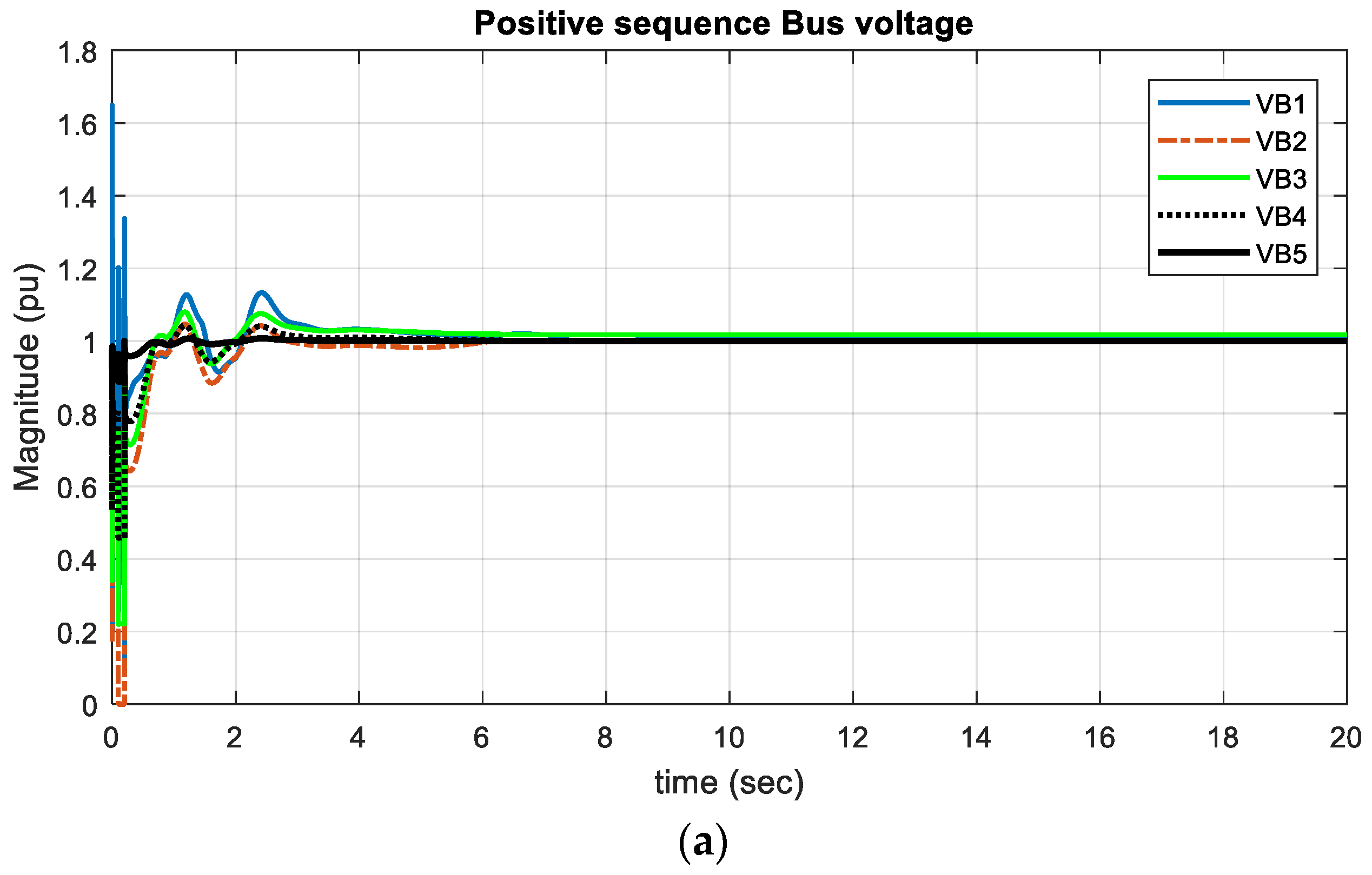
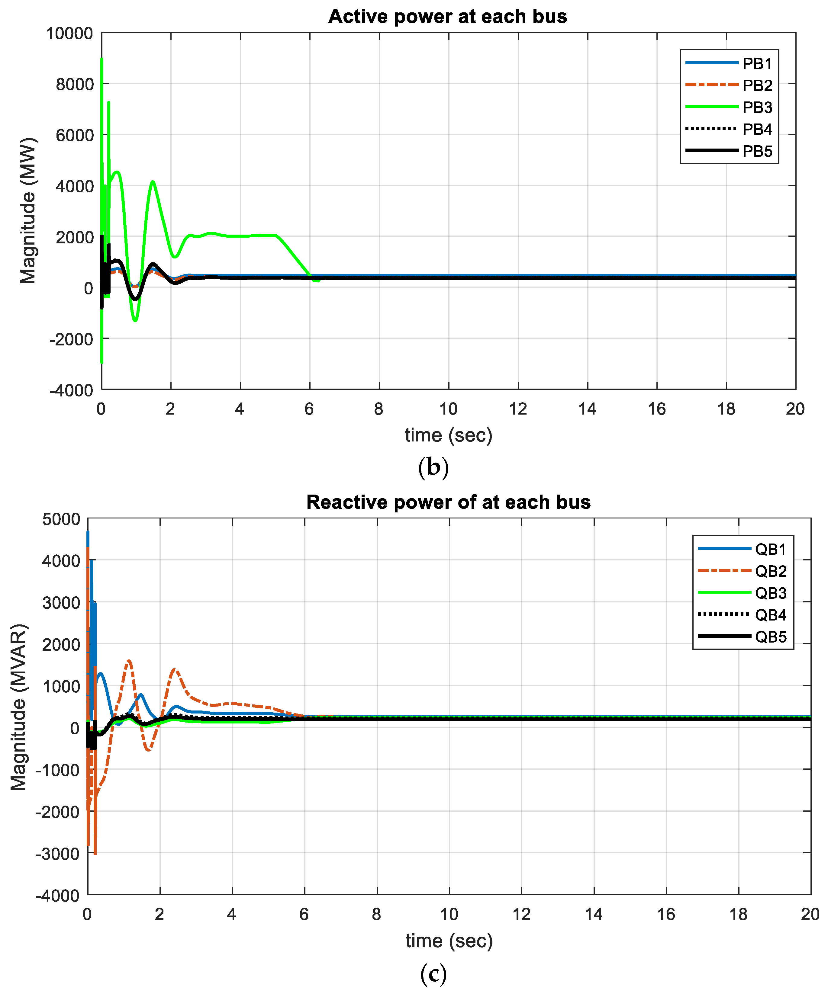
4.2. Simulation Output Results at Each Bus
4.3. Comparison of Proposed Optimization Technique with Other Techniques
4.4. Simulation Results at Different Operating Conditions
4.4.1. Simulation Result at Normal Operating Condition
4.4.2. Discussion of Results at Normal Operating Conditions
4.4.3. Simulation Result at Heavy Operating Conditions
4.4.4. Discussion of Results at Heavy Operating Conditions
4.4.5. Simulation Result at Lightly Loading Condition
4.4.6. Discussion of Result at Lightly Operating Condition
4.5. Main Achievements of the Proposed Method
5. Conclusions
Author Contributions
Funding
Institutional Review Board Statement
Informed Consent Statement
Data Availability Statement
Conflicts of Interest
Nomenclature
| Hz | Hertz |
| IT | Current iteration |
| Maximum number of iterations | |
| Pu | Per unit |
| M, D | Inertia Constant, Damping Coefficient |
| Synchronous Speed of the Generator | |
| δ, ω | Rotor Angle, Rotor Speed |
| Generator Internal Voltage | |
| Field Voltage | |
| AC Bus Reference Voltage | |
| Control Signal of PSS | |
| Id, Iq | dq axes Generator Armature Current |
| Vt | Generator Terminal Voltage |
| KA, TA | Gain and Time Constant of Exciter and Regulator |
| Vb | Infinite Bus Voltage |
| Eigenvalues | |
| σi, ωi | Eigenvalue’s Real Part and Imaginary Part |
| ζ | Damping ratio of mth Eigenvalue |
| T1, T2, T3, T4 | Time Constants |
| K, Tw | Controller Gain and Washout Time Constant |
| Stabilized Voltage | |
| Abbreviations | |
| AC | Alternating current |
| AL | Antlion |
| ALO | Antlion optimization |
| AVR | Automatic voltage regulator |
| DC | Direct current |
| EEP | Ethiopian Electric power |
| FLC | Fuzzy logic controller |
| FLPSS | Fuzzy logic power system stabilizer |
| GA | Genetic Algorithm |
| IEEE | Institute of Electrical and Electronics Engineers |
| kV | Kilo volt |
| kVA | Kilo Volt Ampere |
| kVAr | Kilo Volt Ampere reactive |
| LFO | Lows frequency oscillation |
| MATLAB | Matrix Laboratory |
| MVA | Mega Volt Ampere |
| MVAr | Mega Volt Ampere reactive |
| MW | Mega watt |
| MWh | Megawatt hour |
| NP | Number of operating point |
| PSS | Power system stabilizer |
| PSO | Particle swarm optimization |
| POD | Power oscillation Damper |
| RC | Resistor Capacitor |
| RWs | Random walks |
| SFLA | Shuffled frog leaping algorithm |
| SMIB | Single machine infinite bus system |
| TLBO | Teaching learning-based optimization |
Appendix A
| Generator parameters of the system | M = 8 MJ/MVA D = 4 |
| Exciter type EXST1 data | , |
| Control parameters for generators with governor type UYGOV | |
| Transformer | |
| Transmission line | |
| Operating condition |
| No. | Name | Sn (MVA) | V (kV) | P (MW) | Pmin (MW) | Pmax (MW) | Qmin (MVAR) | Qmin (MVAR) |
| 1 | Beles G1 | 133 | 15 | 80 | 0 | 115 | −130 | 130 |
| 2 | Beles G2 | 133 | 15 | 100 | 0 | 115 | −130 | 130 |
| 3 | Beles G3 | 133 | 15 | 90 | 0 | 115 | −130 | 130 |
| 4 | Beles G4 | 133 | 15 | 100 | 0 | 115 | −130 | 130 |
| No. | From Bus | To Bus | R (pu) | X (pu) | B (pu) | KA | Km |
| 1 | Tana Beles 400 | Bahir Dar 400 | 0.000958 | 0.012159 | 0.37713 | 1341 | 65 |
| Voltage (kV) | Rating (MVA) | R (%) | X (%) | X/R Ratio |
| 400/230 | 133 | 0.176 | 12.045 | 68.44 |
| 400/15 | 133 | 0.215 | 13.5 | 62.79 |
References
- Grebe, E.; Kabouris, J.; Barba, S.L.; Sattinger, W.; Winter, W. Low frequency oscillations in the interconnected system of Continental Europe. In Proceedings of the IEEE PES General Meeting, Minneapolis, MN, USA, 25–29 July 2010; pp. 1–7. [Google Scholar]
- Al-Hinai, A.S.; Al-Hinai, S.M. Dynamic stability enhancement using particle swarm optimization power system stabilizer. In Proceedings of the 2009 2nd International Conference on Adaptive Science & Technology (ICAST), Accra, Ghana, 14–16 January 2009; pp. 117–119. [Google Scholar] [CrossRef]
- Datta, S.; Roy, A.K. Fuzzy logic based STATCOM controller for enhancement of power system dynamic stability. In Proceedings of the International Conference on Electrical & Computer Engineering (ICECE 2010), Dhaka, Bangladesh, 18–20 December 2010; pp. 294–297. [Google Scholar] [CrossRef]
- Rout, K.C.; Panda, P.C. An adaptive fuzzy logic based power system stabilizer for enhancement of power system stability. In Proceedings of the 2010 International Conference on Industrial Electronics, Control and Robotics, Rourkela, India, 27–29 December 2010; pp. 175–179. [Google Scholar] [CrossRef]
- Haghshenas, M.; Hajibabaee, M.; Ebadian, M. Controller Design of STATCOM Using Modified Shuffled Frog Leaping Algorithm for Damping of Power System Low Frequency Oscillations. Int. J. Mechatron. Electr. Comput. Technol. 2016, 6, 2786–2799. [Google Scholar]
- Luo, J.; Bu, S.; Teng, F. An optimal modal coordination strategy based on modal superposition theory to mitigate low frequency oscillation in FCWG penetrated power systems. Int. J. Electr. Power Energy Syst. 2020, 120, 105975. [Google Scholar] [CrossRef]
- Sengupta, A.; Das, D.K. Mitigating inter-area oscillation of an interconnected power system considering time-varying delay and actuator saturation. Sustain. Energy Grids Netw. 2021, 27, 100484. [Google Scholar] [CrossRef]
- Rahman, M.; Ahmed, A.; Galib, M.H.; Moniruzzaman. Optimal damping for generalized unified power flow controller equipped single machine infinite bus system for addressing low frequency oscillation. ISA Trans. 2021, 116, 97–112. [Google Scholar] [CrossRef] [PubMed]
- Trevisan, A.S.; Fecteau, M.; Mendonça, Â.; Gagnon, R.; Mahseredjian, J. Analysis of low frequency interactions of DFIG wind turbine systems in series compensated grids. Electr. Power Syst. Res. 2021, 191, 106845. [Google Scholar] [CrossRef]
- Darabian, M.; Bagheri, A. Design of adaptive wide-area damping controller based on delay scheduling for improving small-signal oscillations. Int. J. Electr. Power Energy Syst. 2021, 133, 107224. [Google Scholar] [CrossRef]
- Mirjalili, S. The Ant Lion Optimizer. Adv. Eng. Softw. 2015, 83, 80–98. [Google Scholar] [CrossRef]
- Thu, W.M.; Lin, K.M. Mitigation of Low Frequency Oscillations by Optimal Allocation of Power System Stabilizers: Case Study on MEPE Test System. Energy Power Eng. 2018, 10, 333–350. [Google Scholar] [CrossRef][Green Version]
- Khodabakhshian, A.; Hooshmand, R.; Sharifian, R. Power system stability enhancement by designing PSS and SVC parameters coordinately using RCGA. In Proceedings of the 2009 Canadian Conference on Electrical and Computer Engineering, St. John’s, NL, Canada, 3–6 May 2009; pp. 579–582. [Google Scholar] [CrossRef]
- Bomfim, A.D.; Taranto, G.; Falcao, D. Simultaneous tuning of power system damping controllers using genetic algorithms. IEEE Trans. Power Syst. 2000, 15, 163–169. [Google Scholar] [CrossRef]
- Shahriar, M.S.; Shafiullah; Rana, J.; Ali, A.; Ahmed, A.; Rahman, S.M. Neurogenetic approach for real-time damping of low-frequency oscillations in electric networks. Comput. Electr. Eng. 2020, 83, 106600. [Google Scholar] [CrossRef]
- Ajami, A.; Armaghan, M. Application of multi-objective gravitational search algorithm (GSA) for power system stability enhancement by means of STATCOM. Int. Rev. Electr. Eng. 2012, 7, 4954–4962. [Google Scholar]
- Hassan, L.H.; Moghavvemi, M.; Almurib, H.A.; Muttaqi, K.M. A coordinated design of PSSs and UPFC-based stabilizer using genetic algorithm. IEEE Trans. Ind. Appl. 2014, 50, 2957–2966. [Google Scholar] [CrossRef]
- Abdel-Magid, Y.L.; Abido, M.A. Optimal Multi objective Design of Robust Power System Stabilizers Using Genetic Algorithms. IEEE Trans. Power Syst. 2003, 18, 1125–1132. [Google Scholar] [CrossRef]


| Parameters | T1 | T2 | T3 | T4 | K |
|---|---|---|---|---|---|
| Minimum | 0.01 | 0.01 | 0.01 | 0.01 | 0.01 |
| Maximum | 1 | 1 | 1 | 1 | 100 |
| Parameters | Tw1 | Tw2 | Tw3 | Tw4 | T1 | T2 | T3 | T4 | T6 | T7 | T8 | T9 |
|---|---|---|---|---|---|---|---|---|---|---|---|---|
| Minimum | 1.15 | 1.15 | 1.15 | 1.15 | 0.01 | 0.01 | 0.01 | 0.01 | 0.02 | 0.02 | 0.02 | 0.02 |
| Maximum | 15 | 15 | 15 | 15 | 1 | 1 | 1‘ | 1 | 2 | 2 | 2 | 2 |
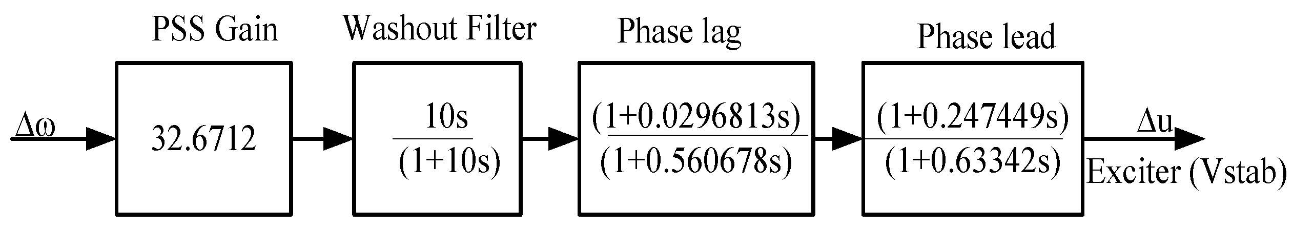
| Parameters | K | Tw (s) | T1 (s) | T2 (s) | T3 (s) | T4 (s) |
|---|---|---|---|---|---|---|
| Optimal values | 32.6712 | 10 | 0.0296813 | 0.560678 | 0.247449 | 0.63342 |
| Parameters | Ks1 | Ks2 | Ks3 | T1 | T2 | T3 | T4 | T6 | T7 | T8 | T9 |
|---|---|---|---|---|---|---|---|---|---|---|---|
| PSS2B | 12.0624 | −1.442 | 16.239 | 0.4217 | 0.8679 | 0.3073 | 0.4475 | 0.665 | 0.1932 | 1.637 | 0.994 |
| Parameters Algorithm | K | Tw | T1 | T2 | T3 | T4 | Sizing Time (s) |
|---|---|---|---|---|---|---|---|
| ALO | 32.6712 | 10 | 0.0296813 | 0.560678 | 0.247449 | 0.63342 | 15.531407 |
| GA | 41.708 | 10 | 0.194398 | 0.212408 | 0.148983 | 0.877625 | 55.909 |
| PSO | 41.708 | 10 | 0.4250 | 0.802737 | 0.107363 | 0.988972 | 106.3817 |
| TLBO | 81.4742 | 10 | 0.166037 | 0.659183 | 0.708986 | 0.444357 | 203.4058 |
| Parameters | Ks1 | Ks2 | Ks3 | T1 | T2 | T3 | T4 | T6 | T7 | T8 | T9 |
|---|---|---|---|---|---|---|---|---|---|---|---|
| ALO | 12.0624 | −1.442 | 16.239 | 0.4217 | 0.8679 | 0.3073 | 0.4475 | 0.665 | 0.1932 | 1.637 | 0.994 |
| GA | 77.5731 | −7.30099 | 8.34627 | 0.194398 | 0.21241 | 0.148983 | 0.87762 | 0.993315 | 0.222622 | 1.33431 | 0.29577 |
| PSO | 62.7183 | −4.43815 | 8.3463 | 0.425003 | 0.80274 | 0.107363 | 0.988972 | 0.247197 | 0.666757 | 0.36123 | 0.059363 |
| TLBO | 34.261 | −8.77915 | 4.46505 | 0.58973 | 0.01311 | 0.80497 | 0.568069 | 0.105715 | 1.7782 | 1.99667 | 0.774753 |
| Parameters | Tw1 | Tw2 | Tw3 | Tw4 |
|---|---|---|---|---|
| ALO | 14.438 | 3.1364 | 9.716 | 2.8045 |
| GA | 2.5121 | 10.658 | 5.03415 | 5.13569 |
| PSO | 1.41823 | 2.56733 | 13.6621 | 13.3838 |
| TLBO | 12.7328 | 4.79597 | 4.91447 | 10.9656 |
| Operating Condition (pu) | Normal Loading P0 = 0.8, Q0 = 0.114, Ut = 1 | Light Loading P0 = 0.2, Q0 = 0.01, Ut = 0.6 | Heavy Loading P0 = 1.20, Q0 = 0.4, Ut = 1.4 |
|---|---|---|---|
| Eigenvalues of base case system | +0.1527 + 9.1627 i +0.1527 − 9.1627 i +1.4242 + 0.0000 i −6.9972 + 0.0000 i −2.8657 + 0.0000 i | −7.0589 + 0.0000 i +1.5345 + 0.0000 i +0.1156 + 5.1410 i +0.1156 − 5.1410 i −2.8400 + 0.0000 i | +0.1320 + 12.5527 i +0.1320 − 12.5527 i +1.5318 + 0.0000 i −6.9952 + 0.0000 i −2.9339 + 0.0000 i |
| Eigenvalues for PSS1B controller | −0.2123 + 8.4810 i −0.2123 − 8.4810 i −5.9644 + 4.8680 i −5.9644 − 4.8680 i +2.8079 + 0.0000 i | +3.3395 + 0.0000 i −1.3107 + 6.8592 i −1.3107 − 6.8592 i −6.9527 + 0.0000 i −3.4574 + 0.0000 i | −2.3738 + 10.6746 i −2.3738 − 10.6746 i −4.1923 + 5.8688 i −4.1923 − 5.8688 i +3.7656 + 0.0000 i |
| Eigenvalues for PSS2B Controller (damping ratio ζ) | −0.2655 + 7.2754 i, 0.03647 −0.2655 − 7.2754 i, 0.03647 −2.5097 + 2.447 i, 0.7161 −2.5097 − 2.447 i, 0.7161 −0.0154 + 0.000 i, 1 | −0.2616 + 4.1837 i, 0.0624 −0.2616 − 4.1837 i, 0.0624 −2.5210 + 2.4518 i, 0.7169 −2.5210 − 2.45181 i, 0.7169 −0.0007 + 0.0000 i, 1 | −0.2701 + 10.1023 i, 0.02673 −0.2701 − 10.1023 i, 0.02673 −2.5038 + 2.4946 i, 0.7084 −2.5038 − 2.4946 i, 0.7084 −0.0182 + 0.0000 i, 1 |
| Maximum Overshoot | Settling Time (s) | |||||||||
|---|---|---|---|---|---|---|---|---|---|---|
| Existing | GA | PSO | TLBO | ALO | Existing | GA | PSO | TLBO | ALO | |
| 0.0182 | 0.0181 | 0.0180 | 0.0180 | 0.0167 | Oscillatory | 6.97 | 11.85 | 14.52 | 4.62 | |
| −2.165 | −1.932 | −1.935 | −1.933 | −1.865 | Oscillatory | 6.27 | 9.78 | 12.23 | 3.95 | |
| 0.017 | 0.0173 | 0.0185 | 0.0180 | 0.016 | Oscillatory | 7.04 | 11.32 | 13.6 | 4.68 | |
| Device | Maximum Overshoot | Settling Time (s) |
|---|---|---|
| Base case | 0.01737 | 20 |
| Conventional PSS | 0.01736 | 10.37 |
| PSS1B | 0.0134 | 6.98 |
| PSS2B | 0.01732 | 4.614 |
| Device | Undershoot | Settling Time (s) |
|---|---|---|
| Base case | −2.048 | 20 |
| Conventional PSS | −2.049 | 10.45 |
| PSS1B | −1.932 | 6.27 |
| PSS2B | −1.910 | 4.14 |
| Device | Maximum Overshoot | Settling Time (s) |
|---|---|---|
| Base case | 2.1298 | 20 |
| Conventional PSS | 2.1958 | 5.417 |
| PSS1B | 2.1899 | 3.2 |
| PSS2B | 2.1610 | 2.910 |
| Device | Maximum Overshoot (pu) | Settling Time (s) |
|---|---|---|
| Base case | 0.017 | 20 |
| Conventional PSS | 0.018 | 10.73 |
| PSS | 0.0173 | 7.04 |
| PSS2B | 0.0161 | 4.49 |
| Device | Maximum Overshoot | Settling Time (s) |
|---|---|---|
| Base case | 0.01748 | 20 |
| Conventional PSS | 0.01747 | 10.35 |
| PSS1B | 0.01738 | 6.98 |
| PSS2B | 0.0168 | 4.77 |
| Device | Undershoot | Settling Time (s) |
|---|---|---|
| Base case | −2.075 | 20 |
| Conventional PSS | −2.074 | 10.37 |
| PSS1B | −1.951 | 6.36 |
| PSS2B | −1.94 | 4.18 |
| Device | Maximum Overshoot | Settling Time (s) |
|---|---|---|
| Base case | 2.0259 | 20 |
| Conventional PSS | 2.1729 | 4.829 |
| PSS1B | 2.150 | 3.2 |
| PSS2B | 2.144 | 2.75 |
| Device | Maximum Overshoot | Settling Time (s) |
|---|---|---|
| Base case | 0.018 | 20 |
| Conventional PSS | 0.0175 | 9.733 |
| PSS1B | 0.0168 | 7.04 |
| PSS2B | 0.0160 | 4.67 |
| Device | Maximum Overshoot | Settling Time (s) |
|---|---|---|
| Base case | 0.01727 | 20 |
| Conventional PSS | 0.01725 | 9.967 |
| PSS1B | 0.0168 | 6.90 |
| PSS2B | 0.01631 | 4.467 |
| Device | Undershoot | Settling Time (s) |
|---|---|---|
| Base case | −2.012 | 20 |
| Conventional PSS | −2.010 | 8.183 |
| PSS1B | −1.920 | 6.25 |
| PSS2B | −1.896 | 4.033 |
| Device | Maximum Overshoot | Settling Time (s) |
|---|---|---|
| Base case | 2.0063 | 20 |
| Conventional PSS | 2.1513 | 4.8 |
| PSS1B | 2.128 | 3.12 |
| PSS2B | 2.125 | 2.8 |
| Device | Maximum Overshoot | Settling Time (s) |
|---|---|---|
| Base case | 0.0175 | 20 |
| Conventional PSS | 0.0170 | 10.32 |
| PSS1B | 0.0169 | 7.01 |
| PSS2B | 0.0162 | 4.43 |
Publisher’s Note: MDPI stays neutral with regard to jurisdictional claims in published maps and institutional affiliations. |
© 2022 by the authors. Licensee MDPI, Basel, Switzerland. This article is an open access article distributed under the terms and conditions of the Creative Commons Attribution (CC BY) license (https://creativecommons.org/licenses/by/4.0/).
Share and Cite
Bayu, E.S.; Khan, B.; Ali, Z.M.; Alaas, Z.M.; Mahela, O.P. Mitigation of Low-Frequency Oscillation in Power Systems through Optimal Design of Power System Stabilizer Employing ALO. Energies 2022, 15, 3809. https://doi.org/10.3390/en15103809
Bayu ES, Khan B, Ali ZM, Alaas ZM, Mahela OP. Mitigation of Low-Frequency Oscillation in Power Systems through Optimal Design of Power System Stabilizer Employing ALO. Energies. 2022; 15(10):3809. https://doi.org/10.3390/en15103809
Chicago/Turabian StyleBayu, Endeshaw Solomon, Baseem Khan, Zaid M. Ali, Zuhair Muhammed Alaas, and Om Prakash Mahela. 2022. "Mitigation of Low-Frequency Oscillation in Power Systems through Optimal Design of Power System Stabilizer Employing ALO" Energies 15, no. 10: 3809. https://doi.org/10.3390/en15103809
APA StyleBayu, E. S., Khan, B., Ali, Z. M., Alaas, Z. M., & Mahela, O. P. (2022). Mitigation of Low-Frequency Oscillation in Power Systems through Optimal Design of Power System Stabilizer Employing ALO. Energies, 15(10), 3809. https://doi.org/10.3390/en15103809