Abstract
From the breakdown of the Kaplan rotor of a hydrogenerator unit and the monitored data collected during its operation before such a failure, this work presents a post-occurrence data analysis in which a previously developed hybrid method based on unsupervised machine learning techniques is applied to detect and diagnose failure before a unit shutdown. In addition to demonstrating the efficiency and capacity of the developed method in an application with real data, the conducted analysis seeks to shed light on the events that occurred at the considered hydroelectric power plant, helping to understand the failure mode evolution and outcome. The results of the fault detection and diagnosis process clearly demonstrated how the evolution of failure modes took place in the analyzed equipment. The detection of potential failures far in advance would support adequate maintenance planning and mitigating actions that could prevent unit breakdown and the consequent damage and financial losses.
1. Introduction
The use of renewable energies and more efficient technologies have become a current solution to meet energy demands while accommodating the decarbonization targets established in the Paris Agreement of 2015 [1]. Among the low-carbon electricity generation technologies, hydropower stands out by producing more than all other renewables-based generation combined, with an installed global capacity of more than 1300 GW and having provided nearly 4500 TWh of power generation in 2020, which corresponds to one-sixth of global electricity generation [1,2].
Furthermore, given the rise of intermittent clean energy sources such as wind and solar, the role of hydropower is shifting to the most powerful and reliable tool capable of stabilizing the electrical grid [3]. The variable demand in the energy market, as well as the limited energy storage capacity of the electrical system, require great flexibility in the operation of Hydroelectric Power Plants (HPP) which, unlike thermoelectric plants, can start-up, increase, and decrease the power output very quickly, allowing prompt adjustments to changes in demand and to compensate for fluctuations in the supply of other electricity sources. Consequently, hydroelectric generators are often operated in a wide range of regimes, which ends up creating additional stress to their components [2,4]. Although HPPs are considered extremely robust facilities, they are not immune from unexpected serious incidents, which end up generating long periods of downtime, considerably high restoration costs, and sometimes representing a serious threat to the life of Operation and Maintenance (O&M) personnel [3,5].
Among all the subsystems and components of a hydroelectric generator, the turbine is probably the one that suffers the most from such aforementioned variation in operational regimes. Basically, there are four main failure modes identified in the literature for a hydroelectric generator turbine: cavitation, erosion, fatigue, and material defects [5]. While the combined effects of sediment erosion and cavitation are the most frequent cause of faults in hydraulic turbines (particularly Kaplan turbines), failures resulting from material defects are considered very rare. Both erosion and cavitation are failure modes that generally develop slowly, bringing relatively mild consequences if properly monitored. On the other hand, material failures can have severe consequences since they often do not allow the previous monitoring of their development and thus occur suddenly.
Having a higher occurrence rate than material defects and consequences much more severe than erosion or cavitation, fatigue may be the failure mode with the higher risk priority among the four failure modes considered. Turbine components that are subjected to repeated alternating or cyclic stresses below the normal yield strength fail progressively due to the development of cracks. The main source of vibration in a hydraulic turbine is the turbulence of the water flow in the turbine blades and eventually, the occurrence of cavitation. The resulting cyclic stresses in the turbine blades end up being transferred to other components because of physical interconnections, causing deformation cycles in practically all turbine components. Furthermore, an overloading of the already affected parts can result in an abrupt failure of the component, making the issue even more serious during operational transients, i.e., machine starting, synchronizing, load changing, shutdowns, load rejections, tripping, failures, or over-speed [5,6].
Faced with the risk of such incidents and aiming to maintain the continuous supply of electricity with minimal operating costs, maintenance activities become extremely relevant and shall be managed to avoid the breakdown of critical components. The most appropriate techniques and the most efficient tools shall be considered to provide the necessary support to maintenance teams in this endeavor, since effective management and maintenance contribute to mitigated physical assets’ risks and business strategy [7], while failures in the processes can be a consequence of poor maintenance [8].
Preventive Maintenance (PM) and Condition-Based Maintenance (CBM) are the most commonly used strategies for maintaining HPP equipment. While the former has proven to be a very effective maintenance method in this type of application, being the basis of most HPP maintenance programs, the latter has gained more prominence in the recent decades, focusing on determining the status of individual components or systems through condition monitoring. In the view of experts, the combination of these two strategies offers the most comprehensive and efficient solution for the maintenance of HPPs [9].
Nevertheless, maintenance techniques continue to evolve, and new tools are available every day, such as machine learning techniques, used to assist in the decision-making process. The role of CBM is fundamental for maintenance planning improvement and the ability to detect potential failures in advance is a key point in this matter.
It is important to have in mind however, hydrogenerators are part of a class of equipment whose access to previously labeled data under fault conditions is generally rare, expensive, or very difficult to obtain. Hydrogenerators are usually customized equipment, designed and built according to the installation that will be carried out, and their projects are rarely reused in different HPPs. Even units in the same plant do not have identical behavior, which means that the development of a certain failure mode does not occur in the same way on different machines.
Due to such features, generally only operational data collected under healthy and certain operational conditions is available, making unsupervised methods, in particular data-based multivariate statistical methods such as Principal Component Analysis (PCA), Partial Least-Squares (PLS), Independent Component Analysis (ICA), and Bayesian Network (BN), more suitable for fault detection and diagnosis in these cases [10,11].
Still, no single method is considered capable of bringing together all the desirable characteristics that a complete approach must contain, such as rapid detection and diagnostic capability, isolability, robustness, adaptability, and multiple fault identification, among others, driving the development of hybrid solutions, in which two or more methods are integrated, complementing and overcoming the limitations of single method strategies [12,13].
In this context, the authors of this work have recently published an article in which a hybrid framework to automate Fault Detection and Diagnosis (FDD) was proposed. FDD is a very important process in CBM strategy, directly influencing maintenance planning and decision making, being a challenging field that has encouraged the development of a wide range of methods and heuristics [14,15,16,17,18].
The proposed framework is based on a combination of two unsupervised machine learning techniques—an extension of the Moving Window Principal Component Analysis (MWPCA) and the Bayesian Network (BN) [12]—that was validated through a case study considering simulated data from a simplified model of a hydrogenerator from a Brazilian HPP, being able to demonstrate the theoretical applicability of the method in a complex engineering system. However, despite the positive results obtained from the analyzed case study, an application with real data was still needed to fully demonstrate the capability of the method.
From such a premise, the present work seeks to verify if the previously published method is capable of correctly detecting and diagnosing a real fault and assess how far in advance this process can be carried out. Furthermore, given the opportunity to better understand the failure mechanisms of hydrogenerators, a discussion about the failure mode development that occurred is also held.
At the beginning of 2020, a severe breakdown of the Kaplan rotor of a hydroelectric generator unit installed in a Brazilian HPP occurred, causing, in addition to a significant cost for its recovery, an inoperative period that lasted until the second half of the same year. The failure occurred during the unit startup and without any prior evidence. Both the monitoring and diagnosis and the Supervision and Data Acquisition (SCADA) systems installed at the plant did not indicate, either during the machine startup or during its steady-state operation in the months that preceded the occurrence, any variation in the monitored parameters that could lead the plant’s O&M team to conclude that they were facing a potential failure.
However, due to the continuous monitoring and storage of several process variables made by the SCADA system, a post-occurrence data analysis could be performed. This analysis, considered the core contribution of the present work, sought to detect and diagnose the possible failure modes that were ongoing in the unit, being carried out by applying the unsupervised machine learning hybrid method previously developed by the authors [12].
The remainder of this work is organized as follows: Section 2 is dedicated to Materials and Methods, presenting both the system and failure descriptions, an overview of the hybrid method applied to the data analysis, and some results and analyzes previously obtained with the method presented under simulated conditions; in Section 3, the monitored data analysis with the fault detection and diagnosis is shown; and finally, in Section 4, the conclusions are presented.
2. Materials and Methods
2.1. System Overview and Failure Description
Hydroelectric generators are equipment whose main function is to transform the potential and kinetic energy of a flow of water into electrical energy, being dependent on two key parameters to perform such task: the available water head, i.e., the height that the water has to fall, and the amount of water flow. These parameters, which are related to the water source available at the plant’s installation site, define the design and selection of the turbine for a hydrogenerator [5].
Conventionally, there are two broad categories of hydraulic turbines: impulse turbines, which include the Pelton, Turgo, and cross-flow designs; and reaction turbines, whose most widely used designs are, in turn, Francis, Kaplan, and propeller. A third relatively new category, which has been increasing in importance recently, is the Very Low Head (VLH) hydropower turbines, which include the axial flow VLH designs and water current turbines [19]. The recent application of VLH hydropower turbines is in line with the development of new technologies and recent efforts to increase and make the operating range of hydraulic turbines more flexible, in addition to minimizing the environmental footprint of hydroelectricity. In this path, new concepts have been incorporated into the traditional use of hydroelectricity, such as variable speed hydropower generation, underwater and underground pumped-storage hydropower, and the use of pumps as turbines in water networks [20,21,22,23,24,25].
Generally speaking, the operating regime of a hydroelectric generator can be classified as steady-state operation and transient-state operation. When in a steady-state condition, the unit operates at a constant head, speed, and power output. The forces acting during this condition tend to be constant in magnitude, direction, and frequency. However, due to abnormalities such as excess pressure pulsations generated in the inlet tube, cavitation, or assembly defects such as misalignments, among others, random non-periodic loads may arise. On the other hand, the operation of a unit during transient conditions occurs when there is a change in head, output power, or flow. In these conditions, induced vibrations do not follow a single pattern, changing their magnitude, direction, and frequency as a function of the water flow in the turbine [6].
Note that the induction of stress in the components of a hydrogenerator can occur both in a steady-state and in a transient regime and not only during the construction and assembly of the unit. Such conditions can be aggravated by the presence of other failure modes, as well as by the constant variation of the generated power, or frequent starts and stops. Furthermore, some turbine types may be more susceptible to failures due to stress fluctuations, both due to their design and operating mode or due to a greater number of elements sensitive to induced vibrations.
Propeller-type turbines, such as Kaplan turbines, fall into this category. Kaplan turbines are designed to operate with a small head and high-water flow [5]. The heart of a Kaplan turbine is the drive mechanism for its rotating blades. The rotor of this type of turbine normally has a rotor hub, in which the rotor blades are coupled, and where the Kaplan mechanism, responsible for the movement of the blades, is located. In this way, the rotor blades can be adjusted to an optimal angle of attack for maximum use of the water flow. This adjustable pitch feature of Kaplan turbines allows efficient operation of this type of turbine over a wide net head range, which can be very useful in sites subject to seasonality that influence the dam water level or the river flow, in the case of run-by-the-river installations such as the one discussed in this work.
Figure 1 presents a schematic representation of a hydrogenerator overview (a) and the Kaplan turbine mechanism main components (b).
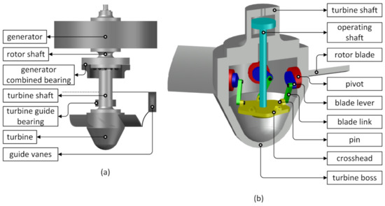
Figure 1.
Hydrogenerator overview (a) and Kaplan turbine mechanism components (b).
The positioning of the rotor blades is controlled by the Speed Governor (SG) system, being carried out in conjunction with the opening of the wicket gate (guide vanes), so that a certain guide vanes’ opening corresponds to a certain inclination value of the rotor blades. Having as its primary function to control the shaft rotation speed by regulating the available water flow in the turbine as a function of the generator output power, the SG is largely responsible for maintaining the synchronism of the hydroelectric generator to the interconnected power grid. To fulfill this function, the SG continually makes small adjustments to the opening of the guide vanes and the rotor blades’ pitch angle, even in a steady-state condition.
In this way, if there is any defect in the wicket gate or turbine blades drive mechanisms, such as looseness, deformations, excessive friction, or locking of moving parts due to the presence of residues, the SG will seek to compensate for such issues, and may significantly increase the loads on its components. In the long run, even small defects of this nature can become big issues, leading to machine failures or even breakdowns if they are not detected and repaired in advance.
In the case of the unit analyzed in this work, the problem remained as a hidden fault for at least 5 months, as will be detailed in Section 4, until the unit broke down during a startup. More precisely, the damaged items that led the unit to its failure were the blade link and the pin that connects it to the blade leaver. The latter, even with a diameter of approximately 2 inches, underwent a complete shear in its transverse section.
Figure 2 presents the blade link and the sheared pin front view (a) and back view (b), in which the pin failure is clear.
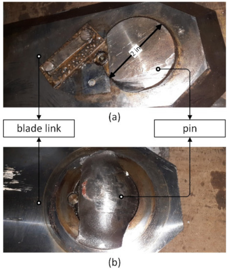
Figure 2.
Blade link and sheared pin: front view (a) and back view (b).
According to reports from the HPP engineering team and the SCADA system data, on 21 January 2020, around 7:00 p.m., the unit’s startup operation began. The unit reached 40% of its maximum power around 9:00 p.m. on the same day and remained in this condition until 10:00 p.m., when it started to have its power reduced and at 2:00 a.m. on 22 January, had a complete shutdown.
It should be noted that from 22 December 2019, to 21 January 2020, the analyzed generating unit remained out of operation for reasons related to the plant’s dispatch schedule, when other units supplied the energy demand. In the period preceding 22 December 2019, in which the unit remained in operation, no anomaly was observed, except for a slight variation in the vibration pattern perceived by the plant’s maintainers team due to the noise emitted by the machine during November 2019. However, no further action was taken since such variation was not considered as an indication of any problem and the generating unit did not have its operation interrupted for this reason at that time. Moreover, as the vibration measurements of the monitoring and diagnosis system were not fully functional during this period, no more detailed analysis could be performed.
After the equipment shutdown, the failure could be immediately associated with the SG system. However, the extent of damage could only be assessed after inspection and disassembly of the equipment, during which a hot spot, probably caused by a short-circuit in the rotor core could be additionally verified. Such fault was unrelated to the generating unit’s SG failure and would be a second failure mode under development in the unit, which, being in an incipient condition, had not been detected previously either.
In circumstances in which two failure modes were identified in simultaneous development in the generating unit, one of which caused the equipment breakdown, a posteriori analysis of the data collected by the SCADA system proves to be valuable, mainly because no signal of alert or alarm has been generated during unit operation. In addition, given the difficulty of obtaining real data that show the variation in the behavior of equipment such as a hydroelectric generator as a function of a failure mode, the analysis of such data becomes a great opportunity to verify if an FDD approach based on machine learning methods would be able to detect and diagnose faults before the machine breaks down. For a better understanding of the method and the found results, the next subsection presents the fundamentals of the applied FDD method.
2.2. Fault Detection and Diagnosis Method’s Fundamentals
The method applied in this work was developed from a hybrid framework whose purpose is to automate the FDD process based on two unsupervised machine learning techniques: an extension of the Moving Window Principal Component Analysis (MWPCA) method and the Bayesian Network (BN) [12]. This framework has three main stages: the system study, the fault detection process, and the fault diagnosis, as presented in Figure 3.
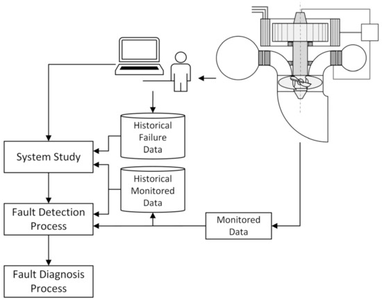
Figure 3.
Fault Detection and Diagnosis Method.
It is proposed that the system study is carried out from a sequence of four tasks in which the system’s knowledge base, necessary for the method execution, is built. In this step, the system components that will be analyzed are defined, the failure modes of each component are identified, which must be correlated with the monitored variables (establishing the detectability of the failure modes), and the information related to the failure modes considered must be collected. In this last task, data such as the failure rate and the moving window necessary to observe the progression of symptoms, intrinsic to MWPCA and directly related to the observability of failure mode symptoms and how they are reflected in the monitored parameters, are obtained.
In the framework’s second stage, the fault detection process is carried out. It includes four scripted tasks designed to automatically run the fault detection process from a computerized system. These tasks are the definition of clusters (composed of a certain number of monitored variables grouped to allow their combined analysis), the construction of the MWPCA-based method input data matrices, the execution of the data analysis, and the categorization of the results obtained from the detection method. At this stage, based on the system and the characteristics of the failure modes, the first scripted task defines the set of monitored variables related to each failure mode. Since an MWPCA-based method is used for fault detection, it is necessary to define a moving window with a fixed length that limits the number of samples analyzed and monitors the variation of data over time [26]. Furthermore, it is necessary to define a reference date from which a time window (the same one used in each cluster) is considered in such a way that the analyzed system is in a healthy and stable condition.
The algorithm of the next two tasks, the construction of the input data matrices, and the execution of the detection method is detailed by the authors in Melani et al. [12]. The result of these tasks consists of a vector of eigenvalues with a dimension equal to twice the number of analyzed variables. Each element of this vector is normalized by the value of the sum of all elements, being the weight of each principal component regarding the total variability of the analyzed data, and the three highest values (called PC1, PC2, and PC3) are considered for the next task.
The last task of this stage, the categorization of the results, is responsible for compiling the current cluster states as an output data object of this process. The possible states for each cluster in the script are “true” or “false”, being the input to the fault diagnosis process. Thus, this task consists of transforming the results of the PCA algorithm into a Boolean value, which characterizes whether the method detected any significant variation in the monitored data for each cluster, i.e., the result of the detection process is a Boolean vector with as many elements as the number of clusters analyzed (being at least the same number of failure modes considered). This transformation consists of verifying the values of PC1, PC2, and PC3 using established limits from a historical series in which the system is within a normal operating condition. If two values, among the three analyzed, exceed their respective limits, the detection result is “true”, or otherwise, “false”.
The fault diagnosis process starts with the construction of the BN graph based on the system information acquired in the first stage of the framework. Two types of nodes must form the graph of the BN: the parent nodes, which represent the failure modes, and the child nodes, which represent the clusters. As described earlier, the number of clusters is greater than or equal to the number of failure modes considered, causing the BN to have at least twice as many nodes as the number of failure modes under study. Each BN node will have two states, “true” and “false”. For nodes related to failure modes, the probabilities of these states indicate the probability of whether the failure has occurred or not. For nodes referring to clusters, on the other hand, these probabilities indicate the probability of detecting a variation in the monitored data. In the construction of the BN, it is also necessary to verify the relationship between the monitored variables, the failure modes, and the clusters. If the observation of a variable is influenced by a certain failure mode, the node related to this failure mode must be connected by an arc to each node that represents a cluster that contains the variable in question. Figure 4 presents an example of a graph of a BN. In this example, the behavior of variables in Cluster 1 is influenced by Failure Modes A and B, while variables in Cluster 3 indicate symptoms of Failure Mode C only. On the other hand, Cluster 2 variables are influenced by the three failure modes simultaneously.
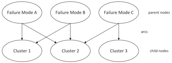
Figure 4.
Example of a Bayesian network graph.
The BN inference can be performed by calculating the posterior probability of a failure mode being true using as input the current clusters’ states. Finally, the process ranks the most likely failure modes to occur based on the posterior probability. Then the BN inference can be performed by calculating the posterior probability of a failure mode being true using the states of the current clusters as input. Finally, the process ranks the most likely failure modes to occur based on the calculated posterior probability.
2.3. Method Previous Results
Before applying the method presented in this work in a real industrial situation, it was compared with other similar methods found in the literature from theoretical requirements and validated from simulated data, as seen in Melani et al. [12].
The comparison of the method to other recent FDD hybrid approaches was performed based on four selected properties: the modeling approach, the necessary input data, the method output, and some additional relevant features. In this way, according to its model, each evaluated method can be classified as supervised data-based (M1), unsupervised data-based (M2), physics-based (M3), or expert knowledge-based (M4). In turn, concerning the necessary input data, the methods can be classified as reliability data-based (I1), when reliability data are used, such as the failure rate of each failure mode; previously labeled monitoring data-based (I2), when data collected previously with the system under a fault condition are needed; or current monitoring data-based (I3), when current monitored data are used. Regarding the model output, the methods can be classified as deterministic (O1), when the diagnosis is obtained deterministically, i.e., the method only defines whether or not a certain failure mode is in progress in the analyzed system; or probabilistic (O2), when the method has as output the likelihood of one or more failure modes being in progress in the analyzed system. Finally, regarding the additional features, the methods can be classified according to the ability to track temporal variations of the monitored system over time (F1) or the ability to detect and diagnose failures not previously observed (F2), i.e., potential failure modes that may occur in the analyzed system but which were not necessarily observed in the operational history of the equipment in question.
On the other hand, in addition to the method applied in this work (MWPCA-BN), the methods analyzed and compared were: the Non-Linear Auto-Regressive Neural Network Model with Exogenous Inputs (NARX) [27]; the Naïve Bayes Classifier combined with BN and Event Tree Analysis (NBC-BN-ETA) [28]; the Multivariate Exponentially Weighted Moving Average Principal Component Analysis combined with BN (MEWMAPCA-BN) [29]; the PCA, BN, and Multiple Likelihood Evidence combination (PCA-T2-BN with MLE) [30]; the Ensemble Empirical Mode Decomposition combined with PCA and Cumulative Sum (EEMD-PCA-CUSUM) [31]; the Residual PCA combined with BN (PCA-R-BN) [32]; the PCA combined with fuzzy theory, data fusion, and BN (PCA-Fuzzy-BN) [33]; the traditional PCA combined with BN (PCA-BN) [34]; the ICA combined with BN (ICA-BN) [35]; Control Charts combined with BN (CC with BN) [36]; and the model-based approach with the Simulation Abnormal Event Management (SimAEM) [37].
The results of this comparative analysis are presented in Table 1.

Table 1.
FDD hybrid methods comparison results.
It can be seen from the results presented in Table 1 that two-thirds of the methods can provide a probabilistic diagnosis, which can be especially advantageous for subsequent decision making by maintenance teams. Half of the methods considered are capable of diagnosing failure modes that were not previously observed in the analyzed system, and only a quarter are those capable of handling nonstationary system data, which is a relevant resource for diagnosing failures in dynamic systems such as hydrogenerators. However, only the method applied in the present work presents all these properties simultaneously, making it the most capable method to detect and diagnose different faults in dynamic engineering systems among the verified approaches.
The ability of the proposed method to detect and diagnose different faults in a dynamic engineering system could be verified from simulations previously carried out by the authors. Considering a simplified model of a hydrogenerator, the framework was implemented and three different failure modes were considered: “generator shaft excessive vibration”, “stator premature degradation of copper insulation”, and “temperature sensor of heat exchanger exit (hot) water does not indicate the actual temperature value”.
To verify the accuracy of the method, 1000 simulations were performed for each of these three failure modes. In each simulation, 350 hours were considered with the system modeled in a healthy condition and 650 hours with the system in a fault condition. Two indices were calculated from such simulations: the Specificity (SPE) and the Sensitivity (SEN) [38]. While the SPE focuses on observations made with the system in a healthy condition, checking the number of true negatives (diagnoses performed with the system in a healthy condition whose result does not indicate any fault in the system), the SEN refers to observations made under fault conditions, verifying the true positives (diagnostics performed with the system in a fault condition whose result correctly indicates the presence of a fault in the system). The higher the SPE and SEN values, the more accurate the method. Furthermore, a high value for the SPE also indicates a robust and reliable method, since in this case, the false alarm rate would be consequently low.
The results obtained indicated a value for the SPE of 0.73, that is, in 73% of the time the system was in a healthy condition, it was correctly diagnosed. On the other hand, the SEN value reached values greater than 0.5 for all three simulated failure modes, reaching a value of 0.85 for the case of the temperature sensor fault. This value would indicate that in only 15% of the time this failure mode was evolving in the system it would not be correctly diagnosed.
Despite the positive results obtained from the simulations, the application of the method under real data conditions was still necessary. Thus, the failure presented in this work and its analysis became a great opportunity for the validation of the method under real conditions, as will be presented in the next section.
3. Analysis and Discussion
As previously presented, the first task of the FDD process built from the proposed framework is the definition of the system components that shall be analyzed. In this case, considering that the failure of the evaluated unit is associated with the SG and, as the functionality of this system is directly associated with the turbine and the generator, the three main systems selected were the turbine, the generator, and the SG. Another determining factor for establishing the subsystems and components considered in the analysis was the availability of monitored data. Since it is not possible to carry out the FDD process of subsystems and components without their monitoring data, only monitored equipment can be analyzed.
Furthermore, the knowledge of failures that previously occurred in the three main systems, especially concerning the a priori probability of these failures, used as an input to the diagnosis process was a determining factor. If any considered failure mode does not have such information, it must be estimated, which inevitably brings a significant increase in the uncertainty of the result.
Thus, based on these considered criteria, the following functional tree, shown in Figure 5, was established.
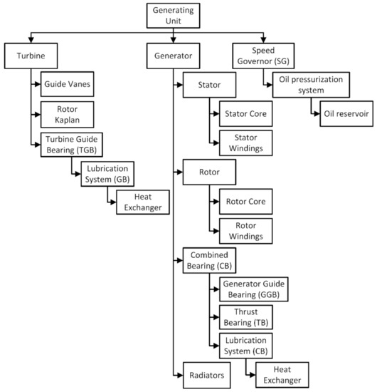
Figure 5.
Functional tree.
For the evaluation proposed in this work, a period of one year was considered for the analysis of monitored data, between 1 January 2019, and 1 January 2020. The choice of this period is based on the search for the incipient identification of the fault, i.e., it is considered as a premise that the failure mode presents itself gradually and during the months before the failure of the unit itself (on 22 January 2020).
Sixty-four measurements were considered as inputs to the fault detection process, plus the active power signal as a determinant variable of the operating condition of the generating unit. Only data that were collected when the unit output power was between 50% and 100% of its maximum value were considered, since most of the time that the unit operated with output power lower than 50% of its maximum value, it was in a transient regime (generally a unit startup or shutdown). Such unstable conditions could be mistakenly identified as fault conditions by the FDD method since the detection process references only data collected in a healthy, stable, and steady-state machine condition [12]. In other words, it is a requirement for the application of the FDD method to use only data collected with the unit in a steady-state condition.
The 64 monitored variables were organized into 10 clusters, used as input in the fault detection process. Each cluster was analyzed individually and its results were applied in the diagnosis process. Furthermore, 8 different failure modes that could affect the functioning of the chosen subsystems and components were considered. Table A1 in Appendix A presents the list of 64 measurements and their relationship with the 10 clusters considered. Table 2 presents the considered failure modes, the components to which such failure modes are associated, the number of failures observed in such components considering the last 5 years, the prior failure rate of each failure mode, and the clusters associated with each failure mode.
Table 2.
Failure modes and clusters relationship.
As presented in Table 2, eight failures were observed in the 5-year period, of which 25% were “guide vanes failures”, 12.5% were “Kaplan rotor failures”, 12.5% were “oil reservoir failures”, 12.5% were “generator failures”, 25% were “combined bearing failures”, and 12.5% were “turbine guide bearing failures”. This 5-year period (from the end of 2013 to the end of 2018) was chosen because it contains reliable information about the unit’s failure history.
Additionally, given the aforementioned difficulty in obtaining failure data for equipment such as hydrogenerators, the failure rate of the “Generator overheating” failure mode was estimated based on the observation of other units similar to the analyzed one.
For the proposed analysis, the reference date considered is 2 January 2019. Regarding the analysis windows, a 240 h time span was considered for clusters 1, 8, 9, and 10, and a 360 h time span for the other clusters.
The values for PC1, PC2, and PC3 over time were obtained between 17 January 2019 (due to the reference window needed to assess the normal condition of each cluster within the defined power output) and 19 December 2019 (the last date on which the unit operated in the defined operating condition before breakdown). Figure 6 shows the results of each considered cluster, with the percentage weight of each main component concerning the total variability of the analyzed data being presented on the ordinate axis and with the time elapsed (in days) after 17 January 2019 on the abscissa axis.
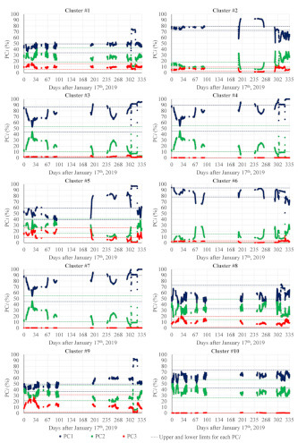
Figure 6.
Cluster analysis results over time. Each graph presents the values of the percentage weight of each main component in relation to the total variability of the cluster analyzed between 17 January 2019 and 19 December 2019.
As mentioned before, in the applied FDD process, the results obtained for the three evaluated PCis can be compiled as an output data object indicating the state in which each cluster finds itself being “true” (T) when at least two of the three analyzed PCi exceed the established limits, or “false” (F) when the opposite occurs and no anomaly is detected. Such limits, in turn, were obtained considering the values calculated for each PCi during the first h hours of analysis, with h, in this case, being the analysis window considered for each cluster. The mean value (PCimean) and standard deviation (PCisd) for each case are obtained from this historical series and are used to define the lower (PCilower) and upper (PCiupper) limits of each PCi, as respectively presented in Equations (1) and (2).
Thus, Figure 7 shows the compiled results of the detection process for all analyzed clusters. Once again, the abscissa axis presents the number of days from 17 January 2019. It is interesting to note that anomalies were detected in all clusters, except for clusters #8 and #10.
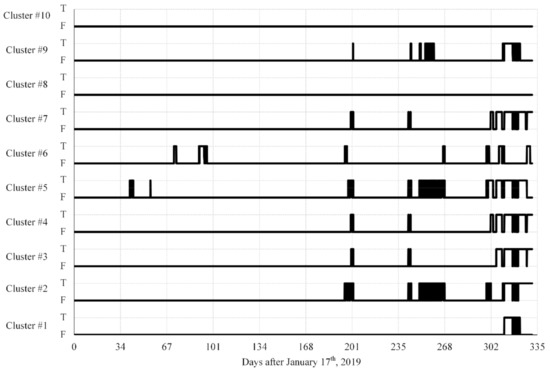
Figure 7.
Detection results over time.
As previously presented, the T and F values of each cluster are the inputs of the BN, used for the diagnosis process. The BN created from the relationship between failure modes and clusters, based on Table 2, is shown in Figure 8.
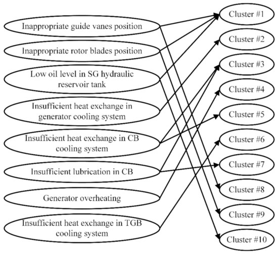
Figure 8.
Bayesian network.
The results of the diagnosis process over time, considering the responses of each cluster shown in Figure 7, applied in turn to the BN shown in Figure 8, considering the a priori probability (presented in Table 2) of each failure mode, are shown in Figure 9. As in Figure 6 and Figure 7, the abscissa axis of the graphs shown in Figure 9 represents the number of days elapsed after 17 January 2019. Analyzing the results of the diagnosis process, it is noticed that 6 of the 8 failure modes considered were diagnosed at some point. The exceptions are failure modes “Inappropriate guide vanes position” and “Low oil level in SG hydraulic reservoir tank”. Furthermore, between November and December 2019, the detection of anomalies became more present, leading to a more evident diagnosis (greater posterior probability) of the failure modes found. Furthermore, note that the diagnosis of failure modes “Insufficient heat exchange in generator cooling system” and “Generator overheating” are strongly correlated, as well as that of failure modes “Insufficient heat exchange in CB cooling system” and “Insufficient lubrication in CB”.
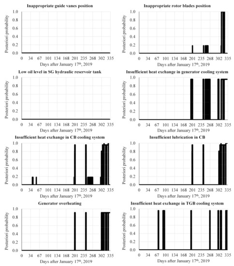
Figure 9.
Diagnosis results over time.
Concerning the presented results, some points can be highlighted. In the case of the SG, for example, whose failure led to the unit’s shutdown, only the failure mode “Inappropriate rotor blade position” was diagnosed during the period considered, and can therefore be fully associated with the variations detected in the behavior of this system. Besides, a variation in the a posteriori probability of this failure mode can be observed over time: from a null probability until the beginning of August 2019, to a probability of 18.3% between August and October 2019, and a value of 99.9% in November. Such variation, together with the fact that the diagnosis becomes constant in mid-November, can be associated with deterioration caused by the presence of the failure mode in the system, i.e., as the failure mode evolved it became more evident. If these results were available during the second half of 2019, it would be clear to the plant’s O&M team that some potential failure would be in development, and the necessary measures could be taken to prevent the equipment from breaking down.
Regarding the diagnosis results related to the generator system (“Insufficient heat exchange in generator cooling system” and “Generator overheating”), it is noted that some factors would be leading to the generator overheating. A fault in the cooling system, as indicated in the results, could be the cause, bringing as a possible consequence the loss of efficiency of the copper insulation and the generation of hot spots due to an electrical failure. It is worth noting that, despite the evidence presented by the detection and diagnosis method for these failure modes, the unit’s SCADA system did not indicate any alarm related to possible issues of this nature. Likewise, when the analyzes presented in this work were in their initial phase, no information about possible failures in the generator was available, even leading the authors to question the results obtained. However, when the unit was disassembled due to the SG failure, evidence of a localized short circuit in the rotor was found, thus confirming the diagnosis generated by the applied FDD method, as presented in Figure 10.
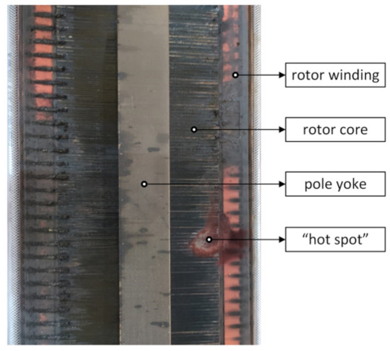
Figure 10.
Rotor core hot spot.
Regarding the combined bearing, the diagnoses process punctually noticed “Insufficient heat exchange in CB cooling system” with a low probability during the months of February and March 2019. Likewise, the same failure mode and the “Insufficient lubrication in CB” failure mode were diagnosed with a high probability, albeit non-continuously, in August and September. During the second half of September and the beginning of October, the failure mode “Insufficient heat exchange in CB cooling system” was diagnosed again, with a low probability, but continuously. As of November, both failure modes considered for this system were identified continuously and progressively, demonstrating some further degradation process related to the lubrication of the combined bearing was in progress. This evidence can be associated with the change in vibration pattern noted by the plant’s staff in November 2019.
Finally, concerning the turbine guide bearing, it is noted that during practically the entire year of 2019 there were sporadic short-lived detections of the considered failure mode, “Insufficient heat exchange in TGB cooling system”. The non-continuity would indicate that such a diagnosis would not actually be associated with the progression of a failure mode, but probably with disturbances in the unit’s behavior. The exception would be in December when the diagnosis became constant in the second fortnight, which may be associated with vibration propagation from the turbine to the rest of the equipment as a consequence of the ongoing failure mode “Inappropriate rotor blades position”. As vibration measurements could not be considered in this case study, the diagnosis of failure modes associated with bearings was compromised due to uncertainties about the observed causes and effects. Even so, it can be said that the failure modes diagnosed in these pieces of equipment are consistent with the problems found in the analyzed unit and reported by the plant’s O&M team.
4. Conclusions
The objective of this work was to verify if a method previously developed by the authors would be able to correctly detect and diagnose faults under real industrial conditions considering a severe failure in a Kaplan rotor of a hydrogenerator unit that occurred at the beginning of the year 2020 and that led to a long period of downtime and significant costs for the unit’s repair. In addition, given the opportunity to better understand the failure mechanisms in hydrogenerators, a discussion on the development of the failure mode that occurred was also held.
The failure in question led to the breakdown of components of the Kaplan rotor blade position regulating system during a unit start up. Evidence collected after disassembly of the unit demonstrates that a “classic” problem of fatigue in components susceptible to vibrations from turbine blades as a consequence of eddy currents was the source of the failure.
Despite the seriousness of the failure, neither the SCADA system nor the monitoring and diagnostic system installed at the plant detected or indicated any potential ongoing failures in the unit. It is noteworthy that vibration measurements in the bearings were not available during the analysis period and could therefore not be considered. However, even without the contribution of such measurements, an FDD method proposed by the authors [12] was applied in a post-occurrence analysis and could successfully not only detect and diagnose the failure mode that led to the unit’s shutdown and breakdown, but also another failure mode associated with a localized short circuit in the rotor core, which was in progress in the unit and similarly, had not been evidenced by the plant’s computational systems. In this second case, only with the disassembly of the generator, the failure mode could be evidenced by the plant’s O&M team.
The detection and diagnosis process results demonstrate how the evolution of failure modes took place in the analyzed equipment, presenting results of potential failures far in advance. For example, the failure mode “Inappropriate rotor blades position”, directly associated with equipment breakdown, was diagnosed in August 2019, that is, more than four months in advance of the failure itself, which only occurred in January 2020. Furthermore, from the end of November 2020, the presence of several failure modes in the system became evident, being even plausible to associate them, such as the issue related to vibration in the bearings and the SG failure modes.
The strong correlation between the failure modes diagnosed by the FDD process and the evidence observed during the operation of the unit, especially considering the failure that led to its shutdown, makes it clear that the proposed method not only has great potential but also had its efficiency proven. It is evident that if the developed system was already available at the plant and the continuous monitoring of the method results by the O&M team was carried out, the unit shut down due to the SG failure and its more severe consequences could have been avoided. This finding makes clear the importance of integrating more modern FDD methods in the daily routine of O&M teams of complex systems, such as hydro generators, to reduce the risks and costs associated with large-scale failures such as the one analyzed in this paper.
Author Contributions
Conceptualization, M.A.C.M., A.H.A.M., R.F.d.S. and G.F.M.d.S.; methodology, M.A.C.M., A.H.A.M., R.F.d.S. and G.F.M.d.S.; validation, M.A.C.M., A.H.A.M., R.F.d.S., G.F.M.d.S. and F.H.H.; formal analysis, M.A.C.M., A.H.A.M., R.F.d.S. and G.F.M.d.S.; investigation, M.A.C.M., A.H.A.M., R.F.d.S., G.F.M.d.S. and F.H.H.; resources, G.F.M.d.S. and F.H.H.; data curation, G.F.M.d.S. and F.H.H.; writing—original draft preparation, M.A.C.M., A.H.A.M. and R.F.d.S.; writing—review and editing, M.A.C.M., A.H.A.M., R.F.d.S. and G.F.M.d.S.; visualization, M.A.C.M., A.H.A.M., R.F.d.S., G.F.M.d.S. and F.H.H.; supervision, G.F.M.d.S.; project administration, G.F.M.d.S. and F.H.H.; funding acquisition, G.F.M.d.S. and F.H.H. All authors have read and agreed to the published version of the manuscript.
Funding
This research was funded by Fundação para o Desenvolvimento Tecnológico da Engenharia (FDTE) and EDP Brasil as part of an ANEEL R&D Project (project number PD-02331-0019/2018).
Institutional Review Board Statement
Not applicable.
Informed Consent Statement
Not applicable.
Data Availability Statement
Some of the data that support the findings of this study can be available from the corresponding author upon reasonable request.
Acknowledgments
The authors thank the support of EDP Brasil.
Conflicts of Interest
The authors declare no conflict of interest. The funders had no role in the design of the study; in the collection, analyses, or interpretation of data; in the writing of the manuscript; or in the decision to publish the results.
Appendix A
Table A1.
Measurements and clusters relationship.
Table A1.
Measurements and clusters relationship.
| Measurements | Clusters |
|---|---|
| Guide vanes position | Cluster #1; Cluster #8 |
| Wicket gate air/oil accumulator pressure | |
| Wicket gate air/oil accumulator level | |
| Rotor blades position Rotor air/oil accumulator pressure | Cluster #1; Cluster #9 |
| SG hydraulic oil reservoir tank level SG hydraulic oil reservoir tank temperature | Cluster #1; Cluster #10 |
| Stator housing hot air temperature | Cluster #2 |
| Radiator 1 cold air temperature | |
| Radiator 2 cold air temperature | |
| Radiator 3 cold air temperature | |
| Radiator 4 cold air temperature | |
| Radiator 5 cold air temperature | |
| Radiator 6 cold air temperature | |
| Radiator inlet water temperature | |
| Radiator outlet water temperature | |
| Radiator outlet water flow | |
| GGB metal temperature 1 | Cluster #3; Cluster #5 |
| GGB metal temperature 2 | |
| TB metal temperature 1 | |
| TB metal temperature 2 | |
| TB metal temperature 3 | |
| TB metal temperature 4 | |
| TB metal temperature 5 | |
| TB metal temperature 6 | |
| TB metal temperature 7 | |
| TB metal temperature 8 | |
| TB metal temperature 9 | |
| TB metal temperature 10 | |
| CB carter oil temperature | |
| CB inlet oil temperature | |
| CB outlet oil temperature | |
| CB heat exchanger water inlet temperature | |
| CB heat exchanger water outlet temperature | |
| CB carter oil level | Cluster #3; Cluster #7 |
| CB carter inlet oil flow | |
| Stator groove 90 phase 2 temperature | Cluster #4 |
| Stator groove 112 phase 1 temperature | |
| Stator groove 139 phase 3 temperature | |
| Stator groove 167 phase 2 temperature | |
| Stator groove 189 phase 1 temperature | |
| Stator groove 216 phase 3 temperature | |
| Stator groove 243 phase 2 temperature | |
| Stator groove 265 phase 1 temperature | |
| Stator groove 292 phase 3 temperature | |
| Stator groove 55–56 upper temperature | |
| Stator groove 55–56 intermediate temperature | |
| Stator groove 55–56 lower temperature | |
| Stator groove 103–104 upper temperature | |
| Stator groove 103–104 intermediate temperature | |
| Stator groove 103–104 lower temperature | |
| Stator groove 157–158 upper temperature | |
| Stator groove 157–158 intermediate temperature | |
| Stator groove 157–158 lower temperature | |
| TGB segment 2 temperature | Cluster #6 |
| TGB segment 4 temperature | |
| TGB segment 5 temperature | |
| TGB segment 6 temperature | |
| TGB oil temperature | |
| TGB heat exchanger inlet water temperature | |
| TGB heat exchanger outlet water temperature | |
| TGB heat exchanger inlet oil temperature | |
| TGB heat exchanger outlet oil temperature |
References
- Quaranta, E.; Bonjean, M.; Cuvato, D.; Nicolet, C.; Dreyer, M.; Gaspoz, A.; Rey-Mermet, S.; Boulicaut, B.; Pratalata, L.; Pinelli, M.; et al. Hydropower case study collection: Innovative low head and ecologically improved turbines, hydropower in existing infrastructures, hydropeaking reduction, digitalization and governing systems. Sustainability 2020, 12, 8873. [Google Scholar] [CrossRef]
- IEA. Hydropower Special Market Report—Analysis and Forecast to 2030; IEA: Paris, France, 2021; Available online: https://www.iea.org/reports/hydropower-special-market-report (accessed on 16 October 2021).
- Yasuda, M.; Watanabe, S. How to avoid severe incidents at hydropower plants. Int. J. Fluid Mach. Syst. 2017, 10, 296–306. [Google Scholar] [CrossRef]
- Frunzǎverde, D.; Muntean, S.; Mǎrginean, G.; Câmpian, V.; Marşavina, L.; Terzi, R.; Şerban, V. Failure analysis of a francis turbine runner. In IOP Conference Series: Earth and Environmental Science; IOP Publishing: Bristol, UK, 2010; Volume 12, p. 012115. [Google Scholar] [CrossRef]
- Dorji, U.; Ghomashchi, R. Hydro turbine failure mechanisms: An overview. Eng. Fail. Anal. 2014, 44, 136–147. [Google Scholar] [CrossRef]
- Luna-Ramírez, A.; Campos-Amezcua, A.; Dorantes-Gómez, O.; Mazur-Czerwiec, Z.; Muñoz-Quezada, R. Failure analysis of runner blades in a francis hydraulic turbine—Case study. Eng. Fail. Anal. 2016, 59, 314–325. [Google Scholar] [CrossRef]
- Holgado, M.; Macchi, M.; Evans, S. Exploring the impacts and contributions of maintenance function for sustainable manufacturing. Int. J. Prod. Res. 2020, 58, 7292–7310. [Google Scholar] [CrossRef]
- Ihemegbulem, I.; Baglee, D. ISO55000 standard as a driver for effective maintenance budgeting. In Proceedings of the 2nd International Conference on Maintenance Engineering, IncoME-II 2017, Manchester, UK, 5–6 September 2017; p. 16. [Google Scholar]
- Selak, L.; Butala, P.; Sluga, A. Condition monitoring and fault diagnostics for hydropower plants. Comput. Ind. 2014, 65, 924–936. [Google Scholar] [CrossRef]
- Alauddin, M.; Khan, F.; Imtiaz, S.; Ahmed, S. A bibliometric review and analysis of data-driven fault detection and diagnosis methods for process systems. Ind. Eng. Chem. Res. 2018, 57, 10719–10735. [Google Scholar] [CrossRef]
- Khorasgani, H.; Farahat, A.; Ristovski, K.; Gupta, C.; Biswas, G. A framework for unifying model-based and data-driven fault diagnosis. In Proceedings of the PHM Society Conference, Philadelphia, PA, USA, 24–27 September 2018; Volume 10, pp. 1–10. [Google Scholar]
- de Andrade Melani, A.H.; de Carvalho Michalski, M.A.; da Silva, R.F.; de Souza, G.F. A framework to automate fault detection and diagnosis based on moving window principal component analysis and bayesian network. Reliab. Eng. Syst. Saf. 2021, 215, 107837. [Google Scholar] [CrossRef]
- Fentaye, A.D.; Baheta, A.T.; Gilani, S.I.; Kyprianidis, K.G. A Review on Gas Turbine Gas-Path Diagnostics: State-of-the-Art Methods, Challenges and Opportunities. Aerospace 2019, 6, 83. [Google Scholar] [CrossRef] [Green Version]
- de Souza, G.F.M.; Caminada Netto, A.; Melani, A.H.d.A.; Michalski, M.A.d.C.; da Silva, R.F. Reliability Analysis and Asset Management of Engineering Systems, 1st ed.; Elsevier: Amsterdam, The Netherlands, 2021; ISBN 9780128235218. [Google Scholar]
- Kaplan, H.; Tehrani, K.; Jamshidi, M. A fault diagnosis design based on deep learning approach for electric vehicle applications. Energies 2021, 14, 6599. [Google Scholar] [CrossRef]
- Isermann, R. Fault-Diagnosis Applications; Springer: Berlin/Heidelberg, Germany, 2011; ISBN 9783642127663. [Google Scholar]
- Habibi, H.; Howard, I.; Simani, S. Reliability improvement of wind turbine power generation using model-based fault detection and fault tolerant control: A review. Renew. Energy 2019, 135, 877–896. [Google Scholar] [CrossRef]
- Chen, X.; Wang, S.; Qiao, B.; Chen, Q. Basic research on machinery fault diagnostics: Past, present, and future trends. Front. Mech. Eng. 2018, 13, 264–291. [Google Scholar] [CrossRef] [Green Version]
- Pandey, B.; Karki, A. Hydroelectric Energy: Renewable Energy and the Envrionment; Ghassemi, A., Ed.; CRC Press: Boca Raton, FL, USA, 2017; ISBN 9781439811672. [Google Scholar]
- Moazeni, F.; Khazaei, J. Optimal energy management of water-energy networks via optimal placement of pumps-as-turbines and demand response through water storage tanks. Appl. Energy 2021, 283, 116335. [Google Scholar] [CrossRef]
- Sambito, M.; Piazza, S.; Freni, G. Stochastic approach for optimal positioning of Pumps As Turbines (PATs). Sustainability 2021, 13, 12318. [Google Scholar] [CrossRef]
- Kougias, I.; Aggidis, G.; Avellan, F.; Deniz, S.; Lundin, U.; Moro, A.; Muntean, S.; Novara, D.; Pérez-Díaz, J.I.; Quaranta, E.; et al. Analysis of emerging technologies in the hydropower sector. Renew. Sustain. Energy Rev. 2019, 113, 109257. [Google Scholar] [CrossRef]
- Pujades, E.; Poulain, A.; Orban, P.; Goderniaux, P.; Dassargues, A. The impact of hydrogeological features on the performance of Underground Pumped-Storage Hydropower (UPSH). Appl. Sci. 2021, 11, 1760. [Google Scholar] [CrossRef]
- Šćekić, L.; Mujović, S.; Radulović, V. Pumped hydroelectric energy storage as a facilitator of renewable energy in liberalized electricity market. Energies 2020, 13, 6076. [Google Scholar] [CrossRef]
- Pérez-Díaz, J.I.; Jiménez, J. Contribution of a pumped-storage hydropower plant to reduce the scheduling costs of an isolated power system with high wind power penetration. Energy 2016, 109, 92–104. [Google Scholar] [CrossRef] [Green Version]
- de Carvalho Michalski, M.A.; de Andrade Melani, A.H.; da Silva, R.F.; de Souza, G.F.; Nabeta, S.I.; Hamaji, F.H. Applying Moving Window Principal Component Analysis (MWPCA) for Fault Detection in Hydrogenerator. In Proceedings of the 30th European Safety and Reliability Conference and the 15th Probabilistic Safety Assessment and Management Conference, Venice, Italy, 1–5 November 2020; Baraldi, P., di Maio, F., Zio, E., Eds.; Published by Research Publishing: Singapore, 2020; p. 8. [Google Scholar]
- Andrade, A.; Lopes, K.; Lima, B.; Maitelli, A. Development of a methodology using artificial neural network in the detection and diagnosis of faults for pneumatic control valves. Sensors 2021, 21, 853. [Google Scholar] [CrossRef]
- Amin, M.T.; Khan, F.; Ahmed, S.; Imtiaz, S. A Novel data-driven methodology for fault detection and dynamic risk assessment. Can. J. Chem. Eng. 2020, 98, 2397–2416. [Google Scholar] [CrossRef]
- Amin, M.T.; Khan, F.; Imtiaz, S.; Ahmed, S. Robust process monitoring methodology for detection and diagnosis of unobservable faults. Ind. Eng. Chem. Res. 2019, 58, 19149–19165. [Google Scholar] [CrossRef]
- Amin, M.T.; Imtiaz, S.; Khan, F. Process system fault detection and diagnosis using a Hybrid technique. Chem. Eng. Sci. 2018, 189, 191–211. [Google Scholar] [CrossRef]
- Du, Y.; Du, D. Fault detection and diagnosis using empirical mode decomposition based principal component analysis. Comput. Chem. Eng. 2018, 115, 1–21. [Google Scholar] [CrossRef]
- Wang, Z.; Wang, L.; Liang, K.; Tan, Y. Enhanced chiller fault detection using bayesian network and principal component analysis. Appl. Therm. Eng. 2018, 141, 898–905. [Google Scholar] [CrossRef]
- Wu, G.; Tong, J.; Zhang, L.; Zhao, Y.; Duan, Z. Framework for fault diagnosis with multi-source sensor nodes in nuclear power plants based on a bayesian network. Ann. Nucl. Energy 2018, 122, 297–308. [Google Scholar] [CrossRef]
- Adedigba, S.A.; Khan, F.; Yang, M. Dynamic failure analysis of process systems using principal component analysis and bayesian network. Ind. Eng. Chem. Res. 2017, 56, 2094–2106. [Google Scholar] [CrossRef]
- Yu, H.; Khan, F.; Garaniya, V. Modified independent component analysis and bayesian network-based two-stage fault diagnosis of Process operations. Ind. Eng. Chem. Res. 2015, 54, 2724–2742. [Google Scholar] [CrossRef]
- Verron, S.; Li, J.; Tiplica, T. Fault detection and isolation of faults in a multivariate process with bayesian network. J. Process. Control 2010, 20, 902–911. [Google Scholar] [CrossRef] [Green Version]
- Olivier-Maget, N.; Hétreux, G.; le Lann, J.M.; le Lann, M.V. Model-Based fault diagnosis for hybrid systems: Application on chemical processes. Comput. Chem. Eng. 2009, 33, 1617–1630. [Google Scholar] [CrossRef] [Green Version]
- Fávero, L.P.; Belfiore, P. Data Science for Business and Decision Making, 1st ed.; Academic Press: Cambridge, MA, USA, 2019; ISBN 978-0-12-811216-8. [Google Scholar]
Publisher’s Note: MDPI stays neutral with regard to jurisdictional claims in published maps and institutional affiliations. |
© 2021 by the authors. Licensee MDPI, Basel, Switzerland. This article is an open access article distributed under the terms and conditions of the Creative Commons Attribution (CC BY) license (https://creativecommons.org/licenses/by/4.0/).