On the Impact of Climate Change on Building Energy Consumptions: A Meta-Analysis

Abstract

The body of literature on climate change impacts on building energy consumption is rising, driven by the urgency to implement adaptation measures. Nevertheless, the multitude of prediction methodologies, future scenarios, as well as climate zones investigated, results in a wide range of expected changes. For these reasons, the present review aims to map climate change impacts on building energy consumption from a quantitative perspective and to identify potential relationships between energy variation and a series of variables that could affect them, including heating and cooling degree-days (HDDs and CDDs), reference period, future time slices and IPCC emission scenarios, by means of statistical techniques. In addition, an overview of the main characteristics of the studies related to locations investigated, building types and methodological approaches are given. To sum up, global warming leads to: (i) decrease in heating consumptions; (ii) increase in cooling consumption; (iii) growth in total consumptions, with notable differences between climate zones. No strong correlation between the parameters was found, although a moderate linear correlation was identified between heating variation and HDDs, and total variation and HDDs. The great variability of the collected data demonstrates the importance of increasing specific impact studies, required to identify appropriate adaptation strategies.

1. Introduction

Climate change is widely recognized as one of the major challenges of our time, as it could be expected to lead to an irreversible transformation of the planet.

The latest Sixth Assessment Report of the Intergovernmental Panel on Climate Change has pointed out that human influence has unequivocally warmed the atmosphere, ocean, and land, by an increase in well-mixed Greenhouse Gas (GHG) concentrations linked to anthropogenic activities [1].

International efforts to tackle climate change were significantly strengthened in the Paris Agreement, adopted at Paris COP21 in 2015, during which 196 countries were required to make an appropriate contribution to climate action. The main goals of this Agreement were to limit global warming below 2 °C compared to pre-industrial levels (ideally to 1.5 °C) and achieve carbon neutrality by mid-century. For instance, to meet its climate and energy targets, the European Union (EU) has committed itself to reducing GHG emissions by at least 20% by 2020, and 40% by 2030 compared to 1990 levels, introducing a wide number of legislative actions.

As a result, several sectors are required to reduce their GHG emissions, carrying out urgent mitigation measures [2]. Among these sectors, a key role is played by the building and construction industry, as it accounts for 36% of final energy use and 39% of energy—and process-related emissions in 2018 [3]. Therefore, improving energy efficiency in buildings has a crucial role in achieving the ambitious goal of carbon-neutrality by 2050 and, at the same time, is considered to be a key factor in the assessment of sustainable living spaces [4]. Several strategies are available to improve the energy efficiency of buildings, including enhancing envelope design parameters, optimizing plan layout, utilizing natural ventilation [5,6]. Furthermore, the introduction of smart technology in buildings is found to be a promising strategy [7].

In addition, buildings are found to be affected by global warming during their lifespan because of the change in outdoor conditions [8], leading to a worsening of energy performance [9] and thermal comfort [10], which also involves high-performance buildings [11]. Therefore, adaptation measures are considered a further key factor to tackle climate change [12], since climate change impacts will continue for centuries, regardless of the efforts to reduce anthropogenic GHG emissions [13]. Nevertheless, relatively little literature can be found concerning climate adaptation for the building industry [14].

The relationship between global warming, energy demand, and GHG emissions has been investigated since the publication of the First IPCC Assessment Report (FAR) in 1990 [15,16]. Nevertheless, the greatest growth in the body of scientific research occurred after the publication of the Third Assessment Report (TAR) in 2001.

According to [17], five major targets can be identified in the research studies on climate change and its impact on buildings: (i) evaluation of the climate change impact on building energy consumption; (ii) adaptation and mitigation measures for buildings against adverse effects of climate change; (iii) models for building retrofitting and renovation to cope with the changing climate; (iv) new tools and methods for future climate projection; (v) uncertainty of climate projection models and their impact on building simulation results.

In this work, the existing literature concerning climate change effects on building energy performance was evaluated, selecting existing articles with a focus on building energy performance in the current and future weather scenarios. This subject has been already investigated by several researchers; nevertheless, although the shift in energy consumption has been proven to be the main consequence of global warming on buildings, the magnitude of this impact can vary significantly, depending on the building type, the geographical context, as well as the methodological approach. As proof of this, the literature reveals a wide range of predicted energy demand changes under projected future weather conditions, resulting in a need for a more comprehensive investigation that utilizes and analyses a large number of studies [18]. Furthermore, a considerable number of variables affect energy evaluation in future climate conditions, reflecting the uncertainties of the input parameters that propagate into the output [19].

A short overview concerning the most common materials and methods adopted to evaluate climate change impacts on buildings is presented in

Table 1. Methods to evaluate climate change impacts on building energy consumption.

	Methodological Phases	Ref.	Input Variable	Variation
1.	Study context	[20]	Geographical context	Different locations characterized by different Heating Degree Days (HDDs) and Cooling Degree Days (CDDs)
		[21]	Building typology	Residential, Commercial, etc.
		[22]	Reference period	Different baseline periods depending on the recorded data availability (TMY2, TMY3, IWEC)
2.	Future weather files prediction	[1,23,24]	Storyline/Representative Concentration Pathways (RCP)	Emissions Scenarios (SRES), Representative Concentration Pathways (RCPs), Shared Socioeconomic Pathways (SSPs)
		[25]	Global Circulation Model (GCMs)	Single or combined GCMs
		[26]	Downscaling technique	Statistical (imposed offset method—i.e., morphing—or stochastic weather method) Dynamical (using Regional Climate Models, RCMs). Hybrid
		[27]	Weather file type	Typical Meteorological Year (TMY), Extreme Cold Year (ECY), Extreme Warm Year (EWY)
		[28]	Study period	Near term, middle term, long term
3.	Energy consumption prediction	[29]	Building model	Dynamical energy simulation model, regression model (degree-days method)

[1,20,21,22,23,24,25,26,27,28,29].

As shown, existing methods encompass three main steps, including the study context identification (geographical context as well as building typology), the prediction of future weather data (based on the selection of emission scenarios, GCMs, downscaling technique, weather file types, and study period), and the prediction of energy consumption comparing future time slices with a reference period (dynamical simulation models, regression model). A series of uncertainties lie in each step, thus making complex the assessment of the relationship between the built environment and the external climate.

Hereafter, a short overview of the three methodological phases is given, to understand the possible input variables behind the research evaluations.

The first step involves the study context identification since the selection of the location and the building typology to be investigated is required.

The second step deals with the prediction of future weather files, which is a crucial point in the reliability of energy consumption forecasts. Broadly speaking, weather projections are mainly based on Global Climate Models (GCMs), extremely sophisticated computer programs which simulate the interactions between the atmosphere, ocean, land surface, snow and ice, the global ecosystem, and a variety of chemical and biological processes [30].

Once they have been validated against past climate observations [31], GCMs are set to run forced by emissions scenarios as initial conditions. The first set of emission scenarios was presented in the IPCC Special Report on Emissions Scenarios (SRES) in 1996 [24], later replaced by the Representative Concentration Pathways (RCPs) [25], along with the so-called Shared Socioeconomic Pathways (SSPs) [1]. These scenarios can be related to different CO₂ concentrations and are adopted as input conditions to run the GCMs. Nevertheless, the direct application of GCMs outputs in building assessment is not recommended since they are characterized by inadequate resolution and bias of the data. Therefore, several methods have been developed to temporally and spatially downscaling GCMs, as reported by Guan [27]. The methods involve statistical (imposed offset method and stochastic weather approach) and dynamical approaches, which are capable to provide weather files suitable for building simulations. On one hand, the imposed offset method imposes the predicted future climate information from the more complex climate models on top of the recorded current reference year weather data and it is most notable in the form of morphing [32], whilst on the other hand, the stochastic weather model, developed by Luo [33] and Adelard et al. [34], is based on an artificial meteorological database. On the contrary, the dynamical approach derives local or regional climate information using a Regional Climate Model (RCM). The advantages and disadvantages of these methodologies have been widely explored and a summary of the main findings is given in

Table 2. Advantages and disadvantages of downscaling methods.

Downscaling Method	Advantages	Disadvantages
Statistical: stochastic method	Allows generating future weather data where historical data are not available [35] The relationships between different weather variables are accounted for in the same way as for baseline data [36] Is possible to simulate extreme weather conditions [23] Is possible to simulate a wide range of feasible climate conditions [23]	Too complex [27] Computationally intensive [27] Difficulties in accurately modeling many climatic variables [27]
Statistical: imposed offset method	Requires minimal computing resources [37] Produces meteorologically consistent weather file, as it is based on historical observations of weather [23,27] The typical reference year weather data for the current climate is also normally available for building simulation [27]	The applicability of any future weather files is constrained by baseline data availability [23], and high quality observed data may be unavailable [37] The future increases in daily maximum and minimum temperature are assumed to be the same as the predicted increases in average temperatures [27] Possible change in solar insolation and wind speed has been ignored [27] If the baseline data to be morphed is already in the form of a TRY, TMY there is also the inherent assumption that any climatic change that occurred between the baseline period of the weather file and baseline period of the climate projections is negligible. [23] Assumes that currently observed relationships will carry into the future [37]
Dynamical	Based on consistent, physical mechanism [37] Not constrained by historical record so that novel scenarios can be simulated [37]	Computationally intensive [37] Requires large volumes of data [37] Requires high level of expertise [37] Due to computational demands, RCMs are typically driven by only one or two GMC/emission scenario simulations [37] May require further downscaling and bias correction of RCM outputs [37] Affected by bias of driving GCM [37]

[23,27,35,36,37]. In addition, a further method can be identified to predict future weather conditions, widely adopted with the degree-day method, which is the extrapolated statistical method. This method uses the approach of extrapolating statistical historical weather data to predict future weather conditions.

The third step deals with the energy consumption prediction, which can be carried out by means of two main approaches: degree-day method and building simulation technique, briefly reviewed in [30]. The degree-day method historically represents a simplified methodology adopted in the earlier studies on climate change impacts [16,38], which assumes a linear relationship between energy demand and the degrees above (below) the cooling (heating) balance point temperature [27]. Future weather conditions were generated based on the projections of the historical climatic data, allowing to predict future building energy consumption (the above extrapolating statistical method). However, the relationship between temperatures and energy consumption is more complicated than the simple linear correlation, highlighting the limitations of this approach which does not consider other weather variables (humidity, solar radiation, wind speed) [39]. Given the limitations of this approach and the development of building simulation technologies, energy simulations are currently the most widespread methodology used to predict the global warming impact on buildings. Building simulation techniques require accurate hourly meteorological input data for energy evaluation, therefore the suitability of weather data is always a crucial point. A comprehensive assessment of existing methods for the creation of current and future weather data suitable for building simulation is given in [23], highlighting various issues with all current and suggested approaches. In addition, a further source of uncertainty is related to the building performance simulation itself.

The major challenges and potential future opportunities in the built environment are well summarized in [40], where drivers determining the future energy consumption of the building sector are examined and their expected evolution is analyzed. These drivers involve: (i) GHG emission and global climate change, (ii) overpopulation and fast urbanization, (iii) urban overheating and local climate change, (iv) high energy consumption, (v) high global environmental impact, (vi) social inequalities, poverty, and ethical issues. This review points out how the expected evolution of these drivers will affect future building consumptions, highlighting that progress in the building sector to deal with them is still slow. The existing literature on the topic reveals a wide range of predicted energy demand changes under projected future scenarios [18]. On one hand, these differences are due to the methodology uncertainties, on the other hand, they are due to the different climatic zones investigated, which are differently affected by climate change [21]. As is clear, each methodological step requires several “input choices” to be made, which can significantly affect the consumption prediction.

Although different methodological approaches have been already overviewed in previous studies [23,41], along with the main impacts of global warming on energy consumption [19,42,43], to the best of our knowledge, quantitative evaluations based on the results of existing studies in terms of energy consumption variation due to climate change have not been ever presented. For these reasons, the present work aims at mapping climate change impacts on building energy consumption from a quantitative point of view, with an attempt to identify potential relationships between energy changes and a series of input methodological variables which could affect them.

More in-depth, the following research problems are addressed:

• What are the main implications of climate change on building energy consumptions according to the existing literature? To what extent do these implications differ between the studies?
• Since several research methodologies can be pointed out, are there any correlations between methodological inputs and research outcomes? In particular, the effects of heating degree-days, cooling degree-days, reference period, future time slices, and emission scenarios (summarized by means of CO₂ concentrations) on the energy consumption variation (heating, cooling, and total) were investigated by statistical techniques.

This paper is organized as follows: the first section reports the review methodology, the second section gives a comprehensive overview of the main features of the selected studies, the third section presents the results of meta-analysis, the fourth section presents the management implication of the results, the fifth section presents the research limitations and future prospect, and in the sixth section the main conclusions are summarized.

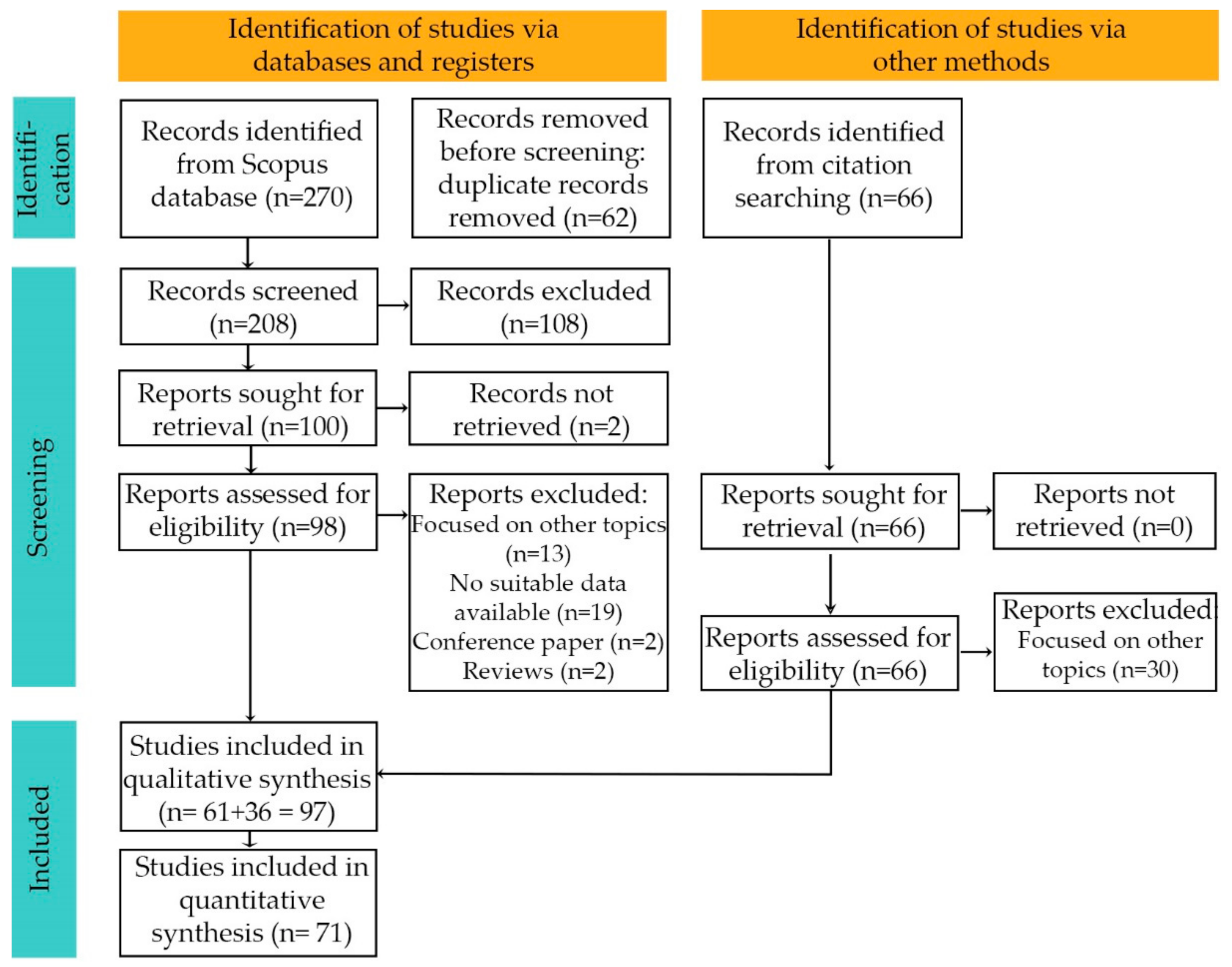
2. Review Methodology

The methodology adopted to conduct the work consists of two main steps. Firstly, a review of the existing literature was performed to collect papers about the research topic, and those suitable for carrying out the quantitative analysis were selected. Secondly, useful data associated with the problem statement were extracted to prepare the datasheet to perform the meta-analysis.

2.1. Studies Selection

The Preferred Reporting Items for Systematic Reviews and Meta-Analyses (PRISMA) guidelines and statements [44] were observed to carry out the literature review, which involves the following five-step procedure: (1) identifying the research question, (2) identifying the keywords, (3) identifying the eligibility criteria, (4) selecting the studies for the qualitative analysis based on the eligibility criteria, (5) selecting the studies for the quantitative analysis.

Based on the research questions, the following keywords were identified to conduct the search:

• To capture articles related to climate change: future weather data; future climate data; climate variables; weather files; weather data; future projections; weather forecasting; climate change impact; climate change; changing climate; future climate condition; future scenarios.
• To capture articles related to buildings: buildings.
• To capture articles related to energy consumption: energy demand, energy consumption, energy performance, performance assessment.

The above keywords were combined to create the Boolean search queries to be applied to the database. The analysis was conducted in the Scopus bibliographic databases, which is considered the most reliable database together with Web of Science [45]. The two databases have been largely compared in several studies, showing that Scopus has a wider coverage of journals and scientific production than Web of Science [46,47]. In addition, Scopus has a faster indexing process than Web of Science, which allows more recent publications to be found by enriching the data collection with updated manuscripts [48]. For these reasons, the analysis was conducted collecting manuscripts retrieved from the Scopus database only, without affecting the validity of the selected sample. Given a large number of results (557 articles), they were narrowed down based on the following inclusion criteria: only papers written in English between 1990 (year of publication of the FAR) and June 2021 were selected, whereas grey literature was excluded. Based on the criteria, the search queries were re-defined, and a further search was run. In addition, both references cited in research reports included in the review and references cited in review reports on a similar topic were examined to identify further studies. Overall, almost 300 articles were identified and submitted to screening. A two-step screening was performed to collect relevant results: firstly, titles and abstracts were examined and excluded if not related to climate change impact on the energy consumption variation. If titles and abstracts were found to be relevant, the full text was assessed for eligibility in detail.

After the screening process, almost 100 were selected and then evaluated to perform the quantitative analysis. Indeed, the findings of a meta-analysis are strictly related to the proper selection of studies. In the selection process of relevant studies, the evaluation criterion was based on the presence of quantitative data concerning energy consumption variation under future climate scenarios, both in numerical and graphical form. Therefore, all the articles reporting qualitative results were excluded. As a result, the number of articles, filtered according to these criteria, was restricted to 71.

The comprehensive process described in this paragraph has been summarised by means of the PRISMA flow diagram [44], as illustrated in Figure 1.

2.2. Data Extraction

Along with the proper selection of studies, the appropriate data extraction is a further crucial point to perform a meta-analysis. After selecting the sample of papers, manual data extraction was carried out and summarised in a matrix, collecting data on the parameters perceived to be relevant. One author (L.M.C.) extracted data from the selected articles, whereas the second author (F.F.) verified them. Then, any contradictions were debated together. The list of the extrapolated data involves the following 14 factors, presented in

Table 3. List of extrapolated data.

Variable		Brief Description
P1.	Building typology	Type of building in accordance with usage
P2.	Location	Reference city/region. When a study was referred to a region, the most representative city was selected.
P3.	Climate zone 1	Climatic zones in accordance with the Köppen-Geiger climate classification system [49]
P4.	Heating Degree Days 1	Calculated based on reference period and location (T = 18 °C)
P5.	Cooling Degree Days 1	Calculated based on reference period and location (T = 18 °C)
P6.	Reference period	Baseline weather file for simulation in current climate conditions
P7.	Emission scenario	Emission scenario adopted for future climate projections
P8.	Downscaling technique	Technique used for generating the future weather files
P9.	Future time slices	Future weather file for simulation in future climate conditions
P10.	CO2 concentration (ppm) 1	Selected in accordance with the emission scenario and the future time slice
P11.	Target	Outcome measured
P12.	Heating consumption variation 1	Percentage variation between heating consumption in the reference period and in the future weather scenario considered
P13.	Cooling consumption variation 1	Percentage variation between heating consumption in the reference period and in the future weather scenario considered
P14.	Total consumption variation 1	Percentage variation between heating consumption in the reference period and in the future weather scenario considered

¹ calculated data.

.

As shown, some data were directly extracted from the papers (P1, P2, P7, P8, P11), allowing further parameters to be calculated (P3, P4, P5, P10). In particular, based on the location investigated, climate zones were selected in accordance with the Köppen-Geiger climate classification system [49]. Then, based on the reference period and the location, heating and cooling degree days were calculated both on the base temperature of 18 °C, by downloading the corresponding weather file (when available). The main sources used to download the reference weather files were the Energy Plus database [50] and the Meteonorm global meteorological database [51]. Furthermore, in accordance with the emission scenario and the future time slice, the corresponding CO₂ concentration (measured in ppm) was selected from [25,52,53]. In addition, other parameters (P6, P9, P12, P13, P14) required processing to be standardized and unified to make the evaluations feasible. Given the multiplicity of reference periods, they have been reduced to three groups (1990, 2000, 2010) according to the last recorded year of the climate series used to generate the reference weather file. Future weather files were also reduced to three future time periods: 2020 (near-term), 2050 (mid-term), 2080 (long-term). Since researchers investigated the influence of climate change on energy consumption based on a different target, i.e., energy demand, net energy, primary energy, thermal loads, or percentage change in energy consumption, data processing was performed to calculate the percentage change in energy consumption for all the studies. In addition, when studies presented the results in a graphical form, the software Origin [54] was adopted to extrapolate numerical data, by means of a graphical interpolation.

2.3. Meta-Analysis

The main purpose of a meta-analysis is to summarise the results—i.e., effect sizes—of different studies answering the same research question. In addition, it allows the exploration of the heterogeneity of results, quantifying the extent of the variance, and thus providing insight into the factors influencing outcomes variability.

In this work, the meta-analysis was conducted according to the well-established methodology given by Borenstein et al. [55], involving three main steps: (i) data preparation; (ii) studies combination; (iii) exploration of heterogeneity. More in-depth, only studies that presented all the parameters described in the previous paragraph were selected, thus reducing the sample from 71 to 19 articles.

Hereafter, the three steps conducted in the analysis are described.

• Data preparation

For each study, the correlation coefficient (r)-with p-values—was calculated since it was chosen as the effect size of the individual study. The effect size is primarily employed in the clinical field; nevertheless, it could represent any relationship between two variables [55]. In this work, the effect size represents the relationship between climate change (measured as the increase in CO₂ concentration) and the energy consumption variation. In particular, as each study presents the variation of energy consumption with respect to three components (heating, cooling, and total variation), three distinct effect sizes were calculated for each study (r_HEATING, r_COOLING, r_TOTAL). Consequently, the results of the meta-analysis will be reported considering separately the three outcomes.

A total of 19 studies were considered, for which the three correlation coefficients and the corresponding 95% confidence interval were defined. Hence, all computations are carried out using the Fisher’s z transformed values [55].

• Studies combination

Since the aim of meta-analysis is to synthesize individual results into a single effect, the outcomes of individual studies need to be weighed in relation to their reliability. Indeed, high-reliability studies have more importance in the combination than low-reliability studies. The process of weighting can be carried out on the basis of a fixed-effect model—which assumes that the true outcome (which is unknown) is the same for all studies—or on the basis of a random-effect model [55]. In the context of the built environment and climate change predictions, studies are not expected to be identical, since a large variety of methodological approaches can be adopted. As a result, a random-effect model was selected to perform the analysis, although it leads to a larger variance, standard error, and confidence interval for the summary effect.

In the random-effect model, the process of weighted consists of two steps, related to two sources of error that occur (within-study V_y and between-study variations τ²). The first step refers to the fixed-effect weighting (w_i), defined as the inverse of the total variance. The second step refers to the random-effect weighting (w*_i), which is the inverse of the sum of the within-study and between-study variance, estimated with the method of moments [55]. Once the random-effect weights were calculated for each study, the combined outcome was calculated as the weighted mean and its standard error is the square root of the variance, which is the inverse of the weights. Then, the combined effect size and the corresponding confidence limits were converted from Fisher’s z metric to correlations [55].

Finally, the resulting data were used to produce three Forest plots (respectively for heating outcomes, cooling outcomes, and total variation outcomes).

• Exploration of heterogeneity

As previously mentioned, the meta-analysis allows the exploration of the heterogeneity of results, quantifying the extent of the variance, and thus providing insight into the factors influencing outcomes variability. Heterogeneity exists when the variation between different studies is above the variation expected by chance and can be evaluated with several approaches [55]. In this work, the index of inconsistency I² proposed by Higgins et al. [56] was adopted, which states low, moderate, and high inconsistency for values of 25%, 50%, and 75% respectively. When evidence of statistical heterogeneity is found, further analyses can be performed to investigate the reasons for this variability. In this work, a correlation analysis was performed in the attempt to identify potential relationships between energy changes and a series of input methodological variables which could affect them.

3. Overview of Studies

According to the inclusion criteria, the quantitative analysis involves a total of 1676 case studies. A list of all included studies along with their main characteristics is given in Appendix A.

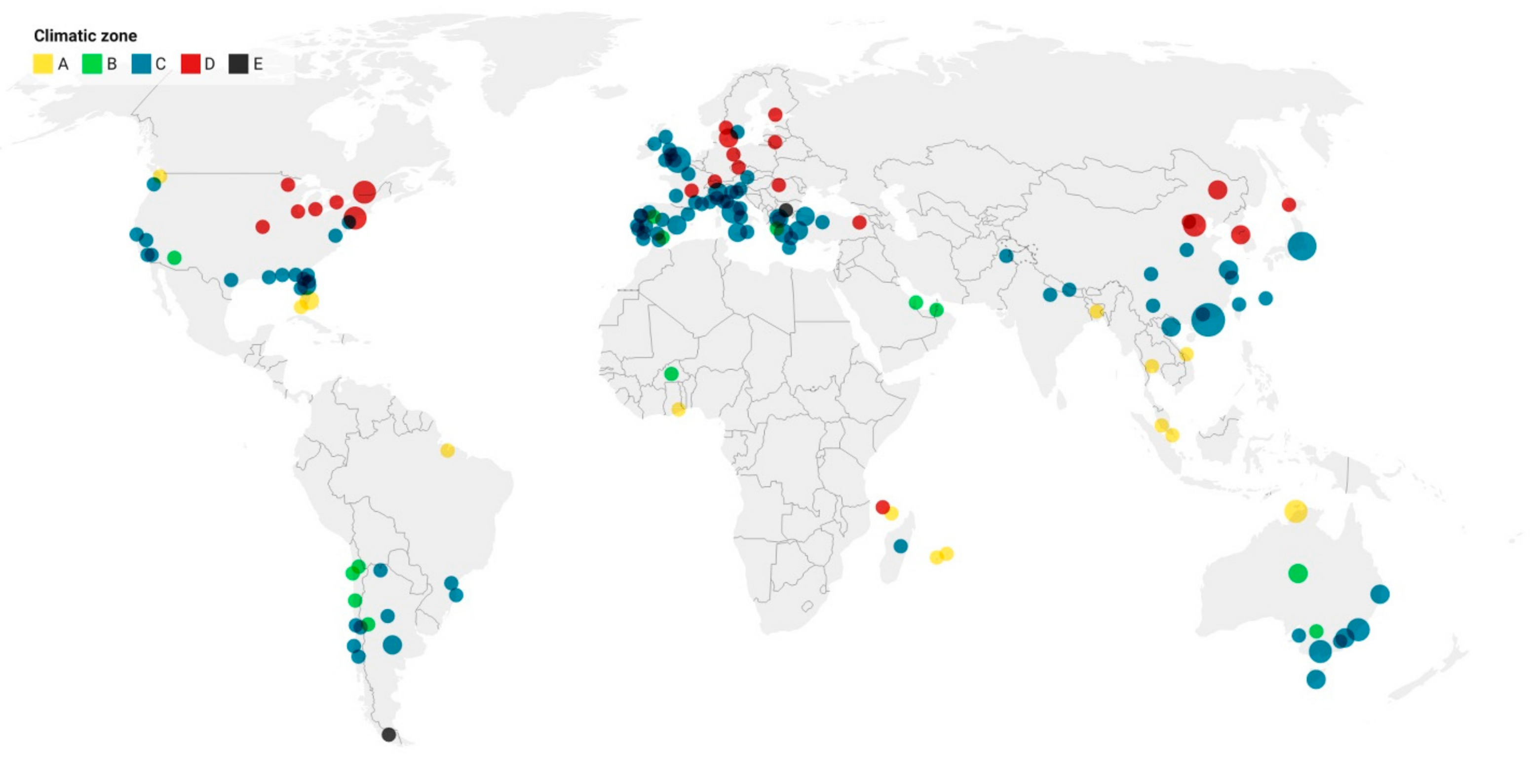
3.1. Geographical Overview

Overall, 46 different countries around the world are covered by the reviewed studies, embracing a total of 146 cities.

From a geographical perspective, the most investigated country appears to be the United States of America (with 9 studies involving US cities), followed by the Honk Kong Special Administrative Region–China (8 studies). Other significant contributions come from Japan, China, and Spain, accounting for 6 studies respectively. Finally, a relevant number of analyses were in the United Kingdom (5 studies), Australia, Canada, and Italy (4 studies each).

An overview of all 146 investigated cities, categorized by the climate zone according to the Koppen-Geiger classification [49], is illustrated in Figure 2. The relative size of the markers is related to the number of studies performed in the location.

As depicted in the figure, the majority of cities lie in the European continent, particularly in the Mediterranean area, which is considered a hotspot for climate change [57]. Then, a significant number of the investigations are found in far-east Asia and on the US east coast, as well as in Australia.

From a climatological point of view, the major literature concerns cities that lie in a temperate climate (type C, 65%), with special emphasis on the Csa zone (hot-summer Mediterranean climate). With 16% of the case studies, the continental climate (type D) is found to be the second most targeted climate zone, followed by tropical climate (type B, 10%), dry climate (type A, 9%), and polar climate (type E, 1%). In addition, a research paper including 102 case studies examines different climate zones and provides the results as an average.

Referring to the individual paper frameworks, it is worth noting that three main categories can be identified in accordance with the selection of the locations to be investigated. Indeed, most research papers are “city level” based (42 out of 71), focusing all the analyses on a specific city. On the other hand, a considerable number of articles (24) are “regional-based”, evaluating several cities located in the same country or region, regardless of the climate zone they belong to. Finally, a limited number of papers (5) are “climate zone” based, selecting cities of different countries which lie in the same climate zone.

3.2. Building Typologies Overview

Although the building typology can significantly affect heating and cooling energy consumption [35], the majority of studies derive their future predictions concerning energy performance on the basis of one/two building types. Indeed, 86% of the investigated research papers (61 out of 71) concerns evaluations on a single building typology, the second group of papers (7%) focuses on two building types, whereas only a few studies (7%) compare more than two building typologies. For instance, a notable exception to the so-called “individual building level” was found in [58], where Huang et al. evaluated the impact of climate change on building energy consumption. They analyzed different building types, and spatial and temporal scales (based on 925 U.S. cities), pointing out the need to assess impacts on a local scale and to tailor adaptation and mitigation strategies to different building types. A further significant contribution was given in [59], where a GIS-based approach to combine climate modeling, building energy simulation, and inventory of building characteristics is presented, aiming at quantifying climate change implications on building energy demand in Los Angeles.

Referring to the building typology, it is worth noting that the greatest emphasis is placed on residential buildings, which account for 40% of the studies, followed by an office building with 26% of papers. By contrast, less attention is given to other building typologies, namely commercial buildings (9%), schools (6%), hospitals (6%), hotels (4%), warehouses (4%), restaurants (3%), and universities (3%).

Referring to the investigated building models, it is worth noting that the reviewed studies based on simulation methodologies can be categorized into four main groups. The first group, the numerous one, focuses on the energy evaluations based on real case studies, which could be validated against measured data. The second and the third groups involve manuscripts which concern typical buildings assumed as representative of the building stock, and building prototypes developed by different standards (i.e., DOE), respectively. Finally, a further group of studies deals with reference buildings in compliance with local standards.

3.3. Methods Overview

Since the considerable number of methodologies adopted, hereafter a brief overview is given. To this aim, available extracted information related to the reference period (P6), the emission scenario (P7), the downscaling technique (P8), and the future time slice (P9)) is summarised in

Table 4. List of extracted parameters related to the methodological framework. The abbreviation n.g. stands for not-given.

	Input Variable	Variation	Frequency (%)	Number of Items
P6	Emission scenario	A2	22	841
		RCP8.5	12	148
		A1B	12	156
		RCP4.5	10	91
		B1	9	89
		No scenario (recorded data)	8	56
		n.g.	7	53
		Other scenarios	19	233
P7	Downscaling technique	Morphing	45	1083
		Offset method	10	145
		Dynamical	7	57
		Stochastic	7	147
		Hybrid	2	10
		No downscaling (recorded data)	13	56
		PCA	5	34
		Other methods	9	141
		n.g.	1	3
P8	Reference period	1990	39	581
		2000	20	580
		2010	37	485
		n.g.	4	30
P9	Future time slice	2020	25	485
		2050	34	659
		2080	31	454
		Recorded data	9	56
		n.g.	1	22

.

In particular, the first column represents the variable, (i.e., the input parameter chosen in the methodological framework), the second column represents the possible parameters of choices, the third column represents the frequency related to the number of papers in which that parameter is chosen. In addition, since several evaluations can be performed in each study, the 71 papers result in 1676 data. Therefore, a fourth column was added to indicate the number of available datasets referring to that parameter.

Once the study context (location and building type) has been defined, the energy performance analyses in future climates can be carried out. As previously said, the appropriate prediction of future weather conditions is a crucial point in the reliability of energy consumption forecasts.

Referring to the downscaling techniques, the reviewed studies encompass all the four main prediction methods pointed out in [27]. The “extrapolated statistical method” seems to be the less frequently adopted method in the selected manuscripts, as it appears in a limited number of studies (4). This method extrapolates statistical historical weather data to predict future weather conditions and is commonly applied in the prediction of building energy consumption trends using degree-day theory, rather than building simulation techniques. Although it historically represents the most applied among the simplified methods, a significant number of assumptions limit the reliability of the results. From a weather prediction perspective, the methodology only accounts for dry bulb temperature, neglecting other weather variables such as humidity, which was found to affect cooling energy consumption in hot seasons [15,60]. Furthermore, from the building perspective, this method requires that building use and heating and cooling systems are constant [27] and does not consider building characteristics–i.e., thermal mass-, leading to potential large deviations in results [26]. In addition, since this approach assumes that a specific indoor temperature is maintained, the adequate selection of the base temperature is challenging, because the assumption of standard temperatures—the most common practice—can lead to inaccurate results. As proof of this, Ismail et al. show that the standard base temperature of 15.5 °C is significantly higher than the real base temperature of the prefabricated building heating by 2.5 °C [30].

Due to these limitations and due to the rapid development of simulation tools, the degree-day method has been rapidly substituted by building simulation techniques, which are adopted in 60 of the selected studies. A wide range of software is available for simulations: the most popular seems to be Energy Plus [i.e., [61,62,63,64]], with its graphical interfaces Design Builder [65,66,67] and OpenStudio [35], as well as TRNSYS [26,60,68,69] or TAS [70,71,72]. Modeling the building behavior allows providing accurate results, even though differences can always be found between real and simulated data.

As previously said, to evaluate energy performance, building simulation software requires hourly weather data. To this aim, global climate models (GCMs), validated against past climate conditions and forced by emission scenarios (or RCPs) are adopted to predict future changes in weather conditions. Nevertheless, these models are characterized by a low level of spatial and temporal resolution, resulting in a need to be downscaled. As a result, any different GCM (or RCM), emission scenario, downscaling technique, or initial conditions leads to a large variety of predictions, encompassing a great number of uncertainties.

From the emission scenarios perspective, which is adopted as input to force GCMs, with 54% of the papers, the use of SRES emission scenarios exceeds the use of RCPs, on the contrary, included in 24% of the studies. Special emphasis is given to the A2 emission scenario, which is involved in the 39% of manuscripts, followed by RCP8.5 involved in 21% of the studies. This focus can be explained by the wide use of web-based weather generator tools, including CCWorldWeatherGenerator [73], which is limited to the A2 scenario, and WeatherShift^TM [74] which is limited to the RCP4.5 and RCP8.5 scenarios. Furthermore, the newly developed SSPs scenarios, that complement RCPs by adding various socioeconomic narratives [53], are adopted in a single study [75].

Referring to the downscaling techniques, the main approaches are summarised in the aforementioned [27], including imposed offset methods, stochastic weather models, and climate models. The literature review shows that there is a heterogeneous use of these methods, with a clear tendency towards one of them. Indeed, among the investigated studies, the imposed offset method is found to be the most adopted approach, accounting for over half of the manuscripts (43 out of 71). More in detail, 3 studies [58,76,77] predict future weather data by adding the expected annual increase in air temperature to a past design reference year data, whilst one study compares three future weather files created by adding annual, monthly, and hourly future temperature rises [71]. Apart from these exceptions, in the remaining 39 papers, the imposed offset method is implemented through the morphing method, developed in [32]. A limited number of manuscripts adopt the last two approaches, which are “stochastic weather models” (6 studies) and “climate models dynamically downscaled” (8 studies), whereas a “hybrid method” is adopted in [78]. Interestingly, almost the totality of the studies is based on a single approach, some of them varying GCMs [69] or emission scenarios, while only 2 papers compare different downscaling techniques [35,79]. An attempt to directly correlate building energy consumption with daily/monthly climate data has been carried out by means of principal component analyses (PCA) and regression analyses in [80,81,82,83]. Briefly, PCA of historical weather data obtained from the local meteorological station and future simulated data from GCMs were used to generate a new composite variable, allowing to explain the long-term variations of the climate variables. Then, regression analysis was performed to elucidate the relationship between the monthly simulated energy consumption and the new composite climatic variable, and the resulting regression model was used to estimate the building energy consumption in the future. In addition, new methodologies are emerging to improve the reliability of the predictions. For instance, a machine learning approach is presented in [84] to improve the weather files required for building energy performance analyses. A bias-correction technique, known as the quantile-quantile method, is applied to decrease the data bias to adapt GCMs to a specific location, and then a hybrid classification-regression model was applied to downscale the bias-corrected GCM data to generate hourly future weather data in a BPS readable format. Furthermore, Chakraborty et al. [75] developed a data-driven explainable Artificial Intelligence (XAI) model which eliminates one of the main shortcomings of existing morphing-based off-the-shelf software. The model allows us to predict continuous daily energy consumptions based on the 21st-century climate change shared socioeconomic pathways scenarios (SSPs).

To analyze the impact of future climate conditions on building energy consumptions, two different types of weather data are required: current weather files to be used as a baseline for assessing actual consumptions, and future weather data files as representative of future scenarios to evaluate future consumption, thus allowing the variation to be calculated. The literature review reveals that a considerable number of studies is still related to the reference period “1990” (39%), derived from weather data observed before 1990 and representative of TMY2 weather files [85], or similar. Therefore, these studies assume obsolete climate files as a baseline and do not consider climate changes that have already occurred in recent years. However, more recent climate files are used as a basis in a great number of studies (37%), which are based on the “2010” reference period, representative of climate files that include data beyond 2000 (i.e., TMY3 [86]). The remaining papers (20%) are based on the “2000” reference period, which is representative of climate files involving data up to 2000 (i.e., IWEC [87]). With regard to future climate scenarios, the reviewed studies carry out assessments on the basis of three-time horizons: 2020 (25%), 2050 (34%), 2080 (31%), whilst a reduced group of manuscripts (8%) bases assessments not only on predicted data, but also on measured data. These observations allow us to create measured weather files, representative of climate trends of recent years, as an average between a range of years [68,88] or as a typical meteorological year [61,72].

4. Results of Meta-Analysis

4.1. Findings Overview

Hereafter, a brief overview of the main findings related to building energy consumption variation is given, based on the reviewed manuscripts. Interestingly, the major of literature investigates climate change impacts on heating, cooling, and total energy consumptions, whilst another part provides information only on total energy consumptions, disregarding individual contributions. In contrast, a limited number of studies focus exclusively on the heating (or cooling) consumption changes, neglecting the overall results. The above-mentioned studies concern the annual consumption changes—which can be expressed in percentage terms-, nevertheless, a minority of studies provide results in terms of rates of increase/decrease in cooling loads per year [60], or energy performance variations in representative months [89,90,91].

Given the considerable number of available data, descriptive statistics were used to summarize the main characteristics of the data set. Data distribution related to heating, cooling, and total energy consumption variation is depicted by means of three boxplots Figure 3a–c and synthetic indices are calculated (

Table 5. Summary of synthetic descriptive indices related to the overall dataset.

	Overall Data	2020	2050	2080
Heating variation	Median	−12.6%	−23.3%	−47.5%
	Mean	−18.83%	−30.28%	−48.72%
	Standard deviation	0.176	0.218	0.272
Cooling variation	Median	28.8%	61.5%	60.9%
	Mean	32.1%	72.3%	204.1%
	Standard deviation	0.366	1.060	11.096
Total variation	Median	2.6%	0.3%	12.0%
	Mean	5.23%	4.73%	20.36%
	Standard deviation	0.345	0.478	0.659

). Each boxplot includes five subgroups representing the main climate zones (subgroups A, B, C, D, E representing climate zones A, B, C, D, E, respectively), along with a further group (All) which involves the overall dataset. Data are represented based on the three future time slices (2020, 2050, 2080).

As expected, referring to the overall dataset (group All), the temperatures’ rise results in two significant consequences on the consumptions trends. On one hand, global warming leads to a progressive decrease in heating consumptions. Indeed, the median value of the variation gradually drops, ranging from −18.6% (2020) to −48.5% (2080). On the other hand, a positive variation in cooling demand can be observed since the median value rises from 28.8% (2020) to 60.9% (2080). As a result, the overall energy consumption steadily grows from 2.6% (2020) to 12% (2080).

As is clear from the graphs, these comprehensive results are biased by the individual contributions of the different climate zones, which are affected by climate change to different extents. The trends described above can be confirmed by investigating each zone individually in detail, however, differences can be outlined by comparing one zone to another. Overall, in comparison with the baseline period, 50% of the data involves a heating reduction ranging between 0–100%, with a considerable variability of data between zones. Except for zone B, considering the representative indices (mean, median), the variation of heating consumption decreases from climate zone A to D. Although it may seem unusual, as zone D is characterized by colder climates, this observation can be explained by the fact that the consumption variation has been calculated as a percentage change. Therefore, in warmer zones (such as zones A), as the heating consumption is lower in the reference period, even a slight variation results in a large percentage increase. Referring to the change in total consumption, climate zone A appears to suffer from the largest increase in consumption, ranging from 14.1% (2020) to 35.1% (2080), while climate zone D seems to experience a slight reduction in consumption, due to a high reduction in winter loads.

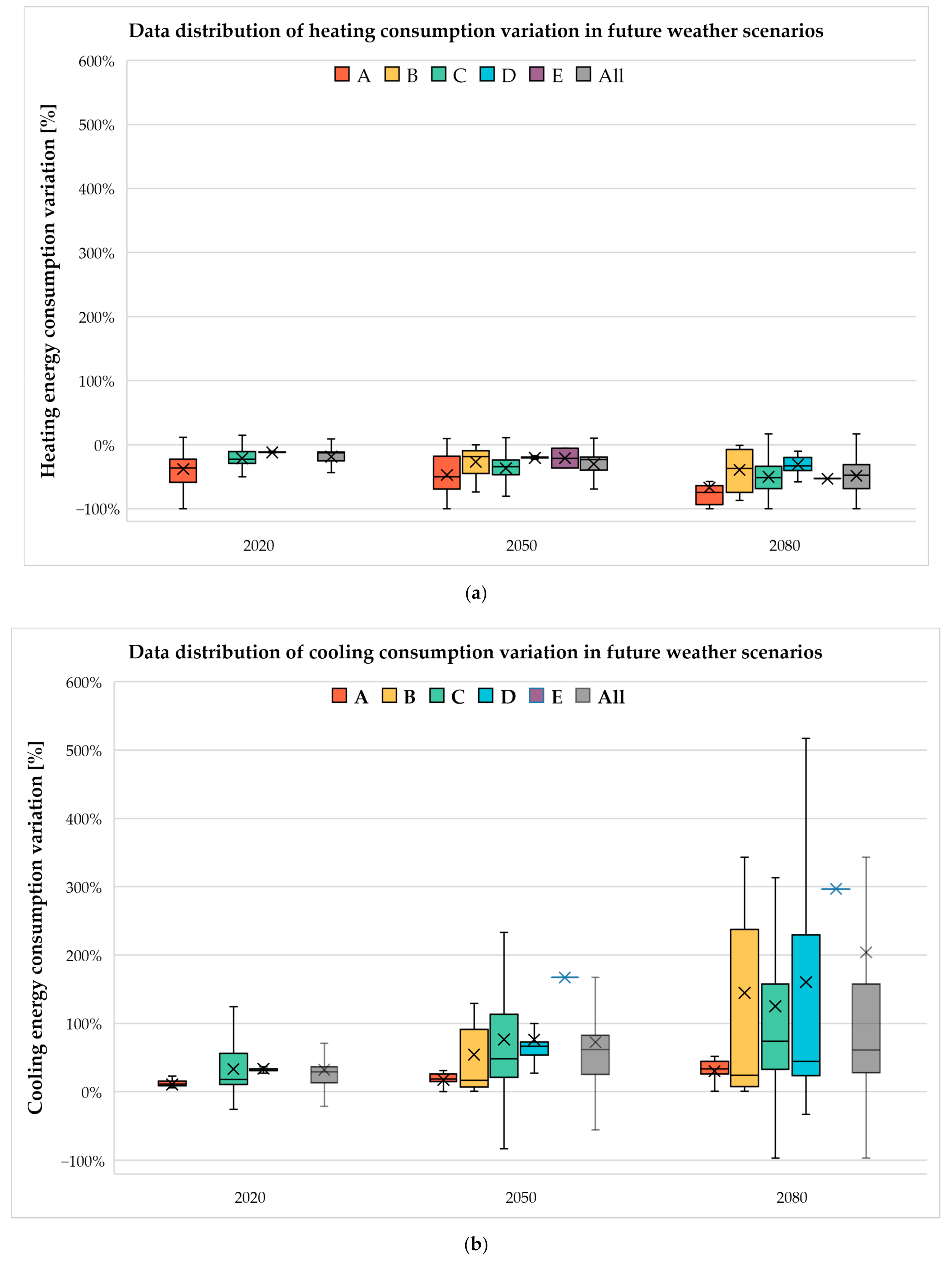
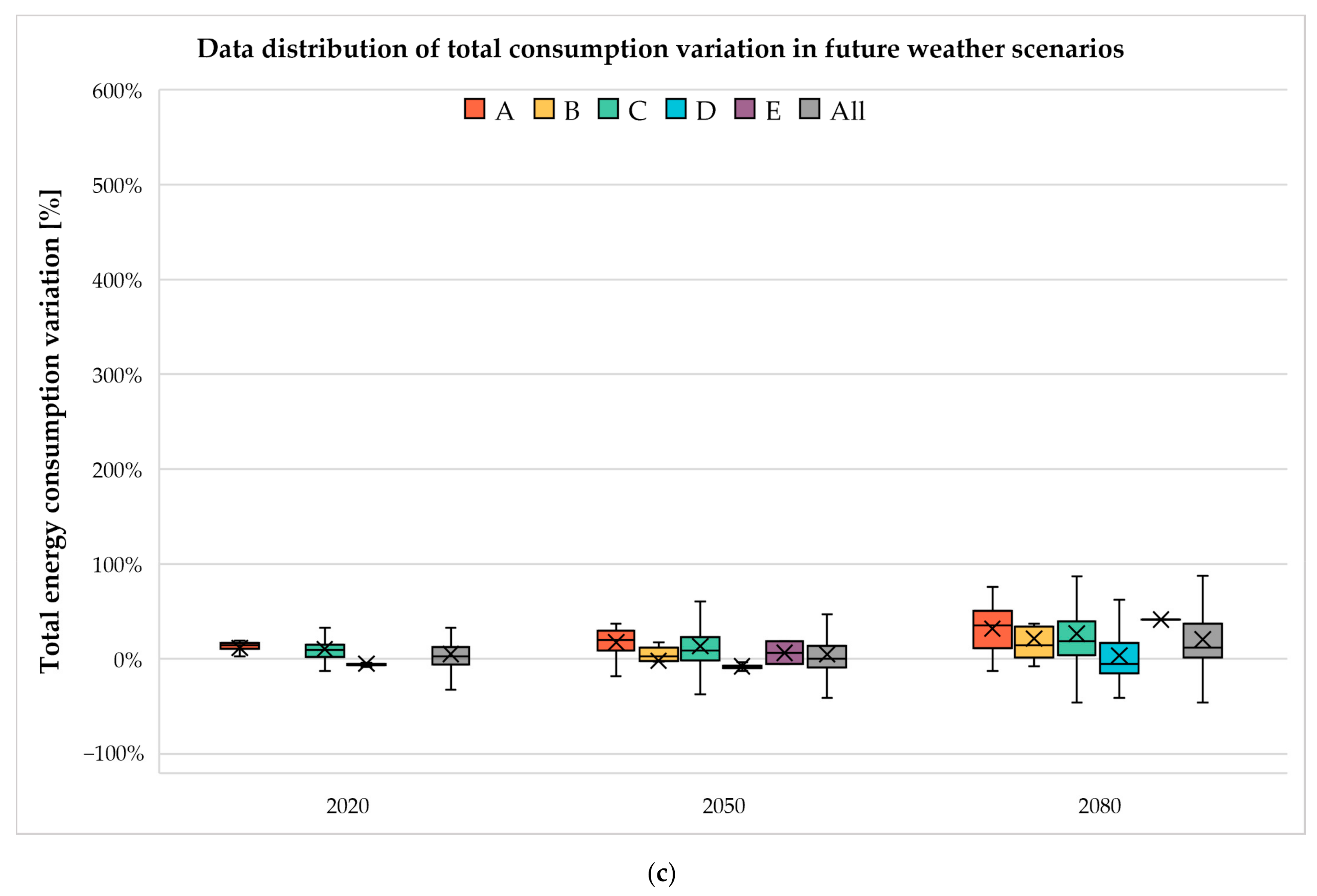
4.2. Statistical Analysis

Hereafter, the Forest Plots of the evaluated studies with the effect size and 95% of the confidence interval are shown (Figure 4).

Three graphs are presented, showing the results referred to the three outcomes considered: (a) heating variation; (b) cooling variation; (c) total variation. More in-depth, the first graph (Figure 4a) represents the effect sizes referred to the relationship between climate change and heating consumption variation. The combined effect size based on the random effect model is −0.62, with a 95% confidence interval ranging from −0.82 to −0.30 (p < 0.001). The second graph (Figure 4b) represents the effect sizes referred to the relationship between climate change and cooling consumption variation, synthesized by a combined effect size of 0.62, with a 95% confidence interval ranging from 0.39 to 0.78 (p < 0.001). Finally, the third graph (Figure 4c) represents the effect sizes referred to the relationship between climate change and total consumption variation, synthesized by a combined effect size of 0.28, with a 95% confidence interval ranging from −0.06 to 0.56 (p < 0.001). A sensitivity analysis concerning the impact of the statistical methods used on the conclusions drawn was performed. Hence, all the analyses were carried out a second time, based on the fixed-effect model. In this case, the combined effect size is equal to −0.76 (95% confidence interval ranging from −0.79 to −0.74) for r_HEATING, 0.63 (95% confidence interval ranging from 0.59 to 0.67) for r_COOLING, and 0.001 (95% confidence interval ranging from 0.066 to 0.068) for r_TOTAL.

A high level of heterogeneity is estimated in all the cases, with an inconsistency index of 96.4% for r_HEATING, 93.1% for r_COOLING, and 94.8% for r_TOTAL. Although in the built environment there are no reference values for interpreting the consistency index, these values can be considered an indication of high heterogeneity, as they are close to the maximum value of 100%. Such a high deviation of studies’ outcomes is not surprising, as research can differ greatly in the adopted methodology, which can influence the obtained results.

For this reason, to understand which methodological parameters could most affect the outcomes, a correlation analysis was carried out. Indeed, if a high level of heterogeneity is found, the focus of the analysis becomes the exploration and explanation of the sources of the variation. The relation between energy consumption variation and a set of methodological input parameters was evaluated by means of statistical techniques. Four input variables were involved in the analysis: P4: Heating Degree Days (HDDs), P5: Cooling Degree Days (CDDs), P6: Reference Period (RP), and P10: CO₂ concentration measured in ppm (CO2); whilst percentage energy consumption variation was evaluated as P12: heating (ΔH), P13: cooling (ΔC), and P14: total variation (ΔT).

A normality test for the variables was graphically performed, by means of q-q plots, which allows us to compare the dataset with normal distribution values for quantiles determined from the dataset itself. Most observations do not follow the reference normal line; therefore, the distributions cannot be assumed as normal. Nevertheless, the central limit theorem (CLT) states that the distribution of sample means approximates a normal distribution as the sample size gets larger, regardless of the population’s distribution [92], therefore if the sample consists of hundreds of observations, the distribution of the data can be ignored and parametric procedures can still be adopted [93]. In addition, data are tested for outliers in XLSTAT software [94] and a limited number of outliers was found. The corresponding data are then checked for possible data errors or measurements problems. Since any unusual condition was found, it was chosen to keep the outliers in the analysis.

Firstly, to evaluate the correlation among the selected variables, the Pearson correlation test was performed in XLSTAT software [94], since it is a parametric test that measures the strength and direction of the linear association between two variables with no assumption of causality. More in detail, this test returns a value between −1 and +1, the former meaning a strong negative correlation and the latter meaning a strong positive correlation, whilst a 0 means that there is no correlation. The calculated Pearson’s r coefficients are presented in

Table 6. Pearson’s r coefficients.

Variable	HDDs	CDDs	RP	CO2	ΔH	ΔC	ΔT
HDDs	1	−0.759	0.120	−0.239	0.458	0.038	−0.445
CDDs	−0.759	1	−0.212	0.161	−0.326	−0.198	0.280
RP	0.120	−0.212	1	−0.082	0.050	−0.129	−0.012
CO2	−0.239	0.161	−0.082	1	−0.415	0.230	0.288
ΔH	0.458	−0.326	0.050	−0.415	1	−0.234	−0.273
ΔC	0.038	−0.198	−0.129	0.230	−0.234	1	0.239
ΔT	−0.445	0.280	−0.012	0.288	−0.273	0.239	1

Abbr. HDDs = Heating Degree Days; CDDs = Cooling Degree Days; RP = reference period; CO₂ = CO₂ concentration; ΔH = heating consumption variation; ΔC = cooling consumption variation; ΔT = total consumption variation.

, with values shown in bold type which indicate statistically significant results, with a p-value p < 0.05.

As depicted, no strong linear correlation can be identified between energy consumption variations and the other input variables, even though moderate linear correlations emerge between heating consumption variation and HDDs (0.458) and CO₂ (−0.415). On the contrary, negative linear correlations can be pointed out between total energy consumption variation and HDDs (−0.445). Nevertheless, the presence of outliers can significantly affect Pearson’s correlation coefficient as well as the line of best fit.

Since our datasets were characterized by a range of outliers, the bivariate correlation among all the variables was assessed using a further test, which is the Spearman rank correlation coefficient (rho), as it allowed the presence of non-linear monotonic relations and non-normality in the datasets, and as it is assumed to be robust to outliers [95]. This is a non-parametric test that measures the strength and direction of the association between two ranked variables. Once again, the rho coefficient can range from −1 (representing a perfect negative monotonic relationship) to 1 (representing a perfect negative monotonic relationship). The calculated rho coefficients are presented in

Table 7. Spearman rho coefficients.

Variable	HDDs	CDDs	RP	CO2	ΔH	ΔC	ΔT
HDDs	1	−0.766	0.237	−0.216	0.497	0.208	−0.588
CDDs	−0.766	1	−0.089	0.034	−0.408	−0.177	0.485
RP	0.237	−0.089	1	−0.140	0.074	0.039	−0.002
CO2	−0.216	0.034	−0.140	1	−0.422	0.190	0.180
ΔH	0.497	−0.408	0.074	−0.422	1	−0.329	−0.337
ΔC	0.208	−0.177	0.039	0.190	−0.329	1	0.181
ΔT	−0.588	0.485	−0.002	0.180	−0.337	0.181	1

Abbr. HDDs = Heating Degree Days; CDDs = Cooling Degree Days; RP = reference period; CO₂ = CO₂ concentration; ΔH = heating consumption variation; ΔC = cooling consumption variation; ΔT = total consumption variation.

. Coefficients shown in bold type indicate statistically significant results, with a p-value p < 0.05, which allows us to accept the null hypothesis (H₀).

As reported, no very strong correlations were found among the variables, although moderate positive correlations can be pointed out between ΔH and HDDs (0.497), as well as a negative correlation between ΔH and CDDs (−0.408). Surprisingly, no obvious correlations emerged between the cooling consumption variation and the other variables, nevertheless, these results do not imply there is no relationship between the variables, rather that there is no monotonic one. Furthermore, significant negative associations can be observed between ΔT and HDDs (−0.588), and to a lesser extent between ΔT and CDDs (0.485). To understand the relationship between the considered variables more in-depth, the most representative scatter plots are reported in Figure 5 and Figure 6.

The data distribution of energy consumption variation with respect to HDDs is illustrated in Figure 5. Three graphs are presented, showing the correlation between HDDs and Figure 5a heating variation, Figure 5b cooling variation, Figure 5c total variation. An upward trend characterizes the relationship between heating consumptions variation and HDDs, confirming the weak positive correlation suggested by the correlation coefficients. Although data appear evenly distributed, a higher concentrated spread of results can be recognized with HDDs values ranging from 0 to 2000, where a numerous number of outliers lies. Notwithstanding, globally, data appear to be distributed with a linear trend, hence a straight line seems to be the best fit (R² = 0.21). Therefore, as the positive gradient of the line, the greater the degree days, the greater the value of variation in heating consumption. However, since the variation is characterized by negative values, this results in a smaller reduction (in absolute value) in heating consumptions with the increase of HDDs.

Since a weak value of a correlation coefficient does not imply the lack of correlation, but rather the absence of linear correlation (Pearson) and the absence of monotonic relationship (Spearman), the distribution of data concerning the variation of cooling consumptions with respect to HDDs was plotted, to identify further suitable relationships. As depicted in Figure 5b, data do not appear to be randomly distributed, but higher variations of cooling consumptions seem to be concentrated in areas where HDDs range from 2000 to 4000. Therefore, polynomial regression is found to be the best fit for the population of data, although with not a strong correlation (R² = 0.108). Finally, data concerning the variation of total consumptions with respect to HDDs are plotted in Figure 5c. Once again, the weak negative correlation suggested by the previously calculated Pearson and Spearman coefficients is confirmed by the points distribution. Indeed, the points follow a negative trend, which can be represented by a straight line with a negative slope (R² = 0.198). Thereby, the increase in total consumption is higher in areas characterized by smaller values of HDDs, decreasing progressively as the HDDs increase, until reaching negative values.

The data distribution of energy consumption variation with respect to CDDs is illustrated in Figure 6. Also, in this case, three graphs are presented, showing the correlation between CDDs and Figure 6a heating variation, Figure 6b cooling variation, Figure 6c total variation. A downward trend characterizes the relationship between heating consumptions variation and CDDs (Figure 6a), which was described by a low value of Pearson coefficient, but a medium value of Spearman coefficient. Even in this case, although the data are well distributed, a higher concentration of results between 500 and 1000 CDDs can be found, whereas a considerable number of outliers characterized the whole chart. Despite that, the data distribution suggests a negative trend, with a reduction in heating consumption as CDDs increase. Assuming a linear relationship between the two variables, it would be characterized by an R² = 0.106, confirming the low value of the Pearson coefficient. Referring to Figure 6b,c, the widespread distribution of the data does not allow a clear relationship between the variables to be identified. Nonetheless, the relationship between cooling consumption variation and CDDs appears to be on a downward trend, with a high number of outliers for CDDs values ranging between 0 and 500. On the contrary, the variation of total consumption does not seem to follow any trend, as it is characterized by highly scattered values and thus does not allow us to find a significant correlation.

5. Management Implications

The quantitative analysis reveals that climate change will have a strong impact on energy consumption in buildings, requiring urgent policy action to be taken. Indeed, albeit to different extents, the implications of global warming will affect buildings across the whole planet, requiring global efforts to tackle dramatic consequences. As shown, although climate change leads to a slight decrease in heating consumption, it also leads to a significant increase in cooling consumption, resulting in overall growth in total building consumption. Therefore, this overall growth results in an increase in direct CO₂ emissions, since fossil fuels are still the most widely used resource for satisfying the buildings’ thermal needs [96]. In addition, cooling energy consumption strongly affects the increase of the peak electricity demand, requiring one to build additional power plants to satisfy the extra needs for electricity [97].

The variability of the data suggests that specific studies need to be carried out to accurately evaluate the impact of global warming on the buildings under investigation and to avoid ineffective measures being taken. Nevertheless, as the trends of changes in consumption are quite similar, some general actions can be pointed out, according to [98]:

• Mitigate global and local climate change.
• Increase of energy savings, improving building performance considering future weather conditions, and designing buildings with the minimum possible cooling needs.
• Improve the efficiency of mechanical air conditioning and alternative cooling technologies.

Obviously, to achieve these objectives the adoption of green policies and a considerable increase of investments are needed, even though no clear engagements towards the adoption of such policies are undertaken [99].

6. Research Limitation and Future Prospect

While in clinical research, systematic reviews and meta-analyses are a basic part of evidence-based medicine, with strict protocols to be respected [100], in the field of the built environment quantitative assessments are still found to be rare [101], whereas qualitative reviews are prevalent. For this reason, specific methodologies are still not well established, while attempts to adapt clinical methodologies are common. The first limitation of this work is the lack of a publication bias assessment, which could affect the results achieved. In addition, the low number of studies available, as well as some missing data in the studies, narrow down the sample of manuscripts allowing the meta-analysis to be performed. Finally, the lack of other meta-analyses on this topic does not provide a basis for comparison with the obtained results.

The aim of this work was to conduct a meta-analysis to compare and combine the results of various studies measuring climate change impacts on building energy consumptions. The main results show a great heterogeneity of data, therefore the potential influencing factors related to the methodology adopted were explored by statistical techniques. The results did not show strong correlations between the analyzed factors and the outcomes, therefore further studies to investigate the source of heterogeneity are required. In addition, some aspects of the meta-analysis methodology should be further investigated in future studies, to improve its application in the built environment field.

7. Conclusions

In this work, a review of the state of the art concerning the impact of climate change on building energy consumption was performed, addressing the problem from a quantitative point of view. Indeed, based on a set of inclusion criteria related to the problem statement, a sample of research papers was selected, and their main characteristics were extracted and summarised in a matrix, collecting data on the parameters perceived to be relevant. Thus, these variables were used as a basis to perform quantitative analyses.

The main findings of this paper can be summarised as follows:

• From a geographical point of view, the spread of the studies does not appear to be homogeneous across the planet, but rather a preponderance of investigations was identified in Europe, far-east Asia, and the eastern United States, with a special emphasis on climate zone C (65% of studies). Further research should be conducted by encompassing other climate zones, since climate change does not affect the planet uniformly.
• The literature on the impacts of climate change still appears to be related to specific building types such as residential (40% of studies) and office buildings (26%), neglecting other building typologies. Nevertheless, since climate change adaptation measures will be needed in the coming years, regardless of the efforts to tackle global warming, further building types need to be studied and specific adaptation strategies identified. Indeed, each building type presents specific characteristics that do not allow it to be compared with the other, and adaptation measures should be tailored to ensure the best performance.
• Several considerations can be highlighted about the employed methodologies. Firstly, most studies still adopt as current climate files climate, files based on weather data observed before 1990 (37% of studies), thus obsolete and not suitable for representing the current climate which is already affected by climate change. Accordingly, the availability of weather files based on more recent data representative of the actual climate is essential to conducting reliable assessments. Secondly, the reviewed studies appear to be largely based on the SRES emission scenarios (54% of studies), which are now outdated. As impact assessments are strongly influenced by the emission scenario selected to generate future weather files, the spread of investigations based on the new IPCC scenarios is desirable. Finally, regarding downscaling techniques, the imposed offset method (which includes the morphing method) is undoubtedly the most widespread approach, accounting for more than half of the manuscripts (61% of studies), while the use of the stochastic and dynamical methods is found to be still limited. Given the high level of uncertainty in predictive analyses, further studies involving not a single approach, but rather the use of different methodologies should be conducted.
• Climate change is expected to be responsible for a deep change in the energy consumption of buildings. Indeed, according to the analyses carried out—which include a sample of 1671 data collected from the manuscripts-, the increase in temperatures will globally lead to: (i) a reduction in heating consumptions from −12.6% (2020) to −47.5% (2080); (ii) an increase in cooling consumptions from +28.8% (2020) to +60.9% (2080); (iii) a growth in total consumptions from +2.6% (2020) to +12% (2080). Clearly, these overall results are influenced by the different climate zones involved, which are affected by climate change to different extents. Climate zone A seems to suffer the greatest rise in energy consumption, while zone D appears to be the least affected.
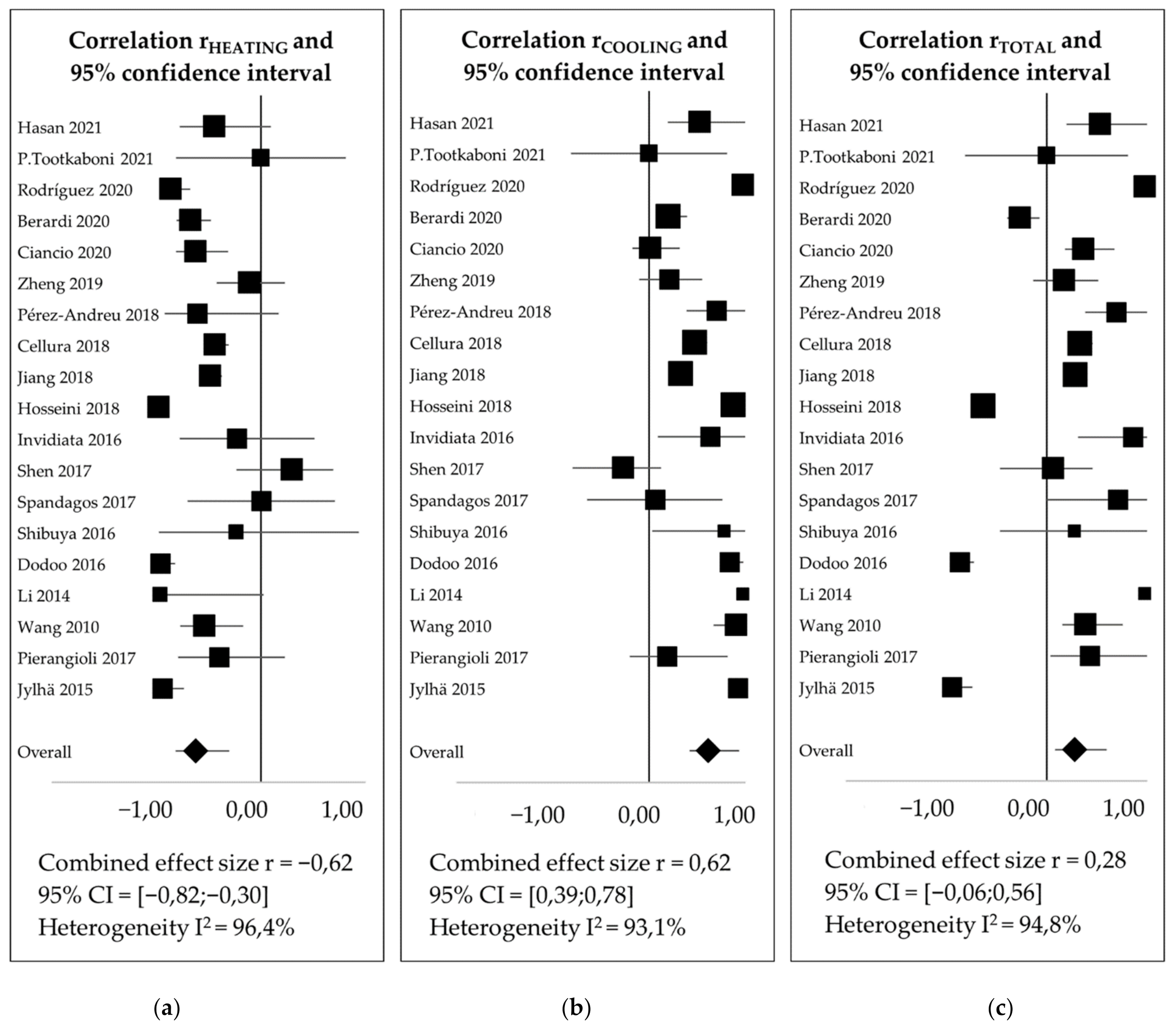
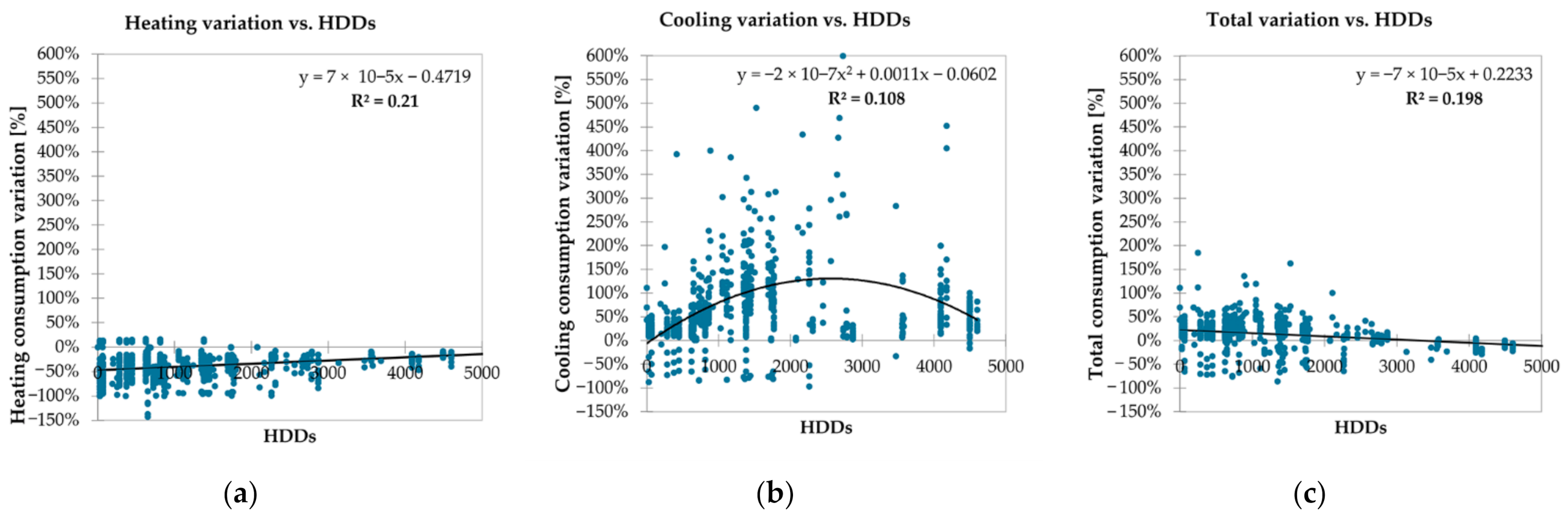
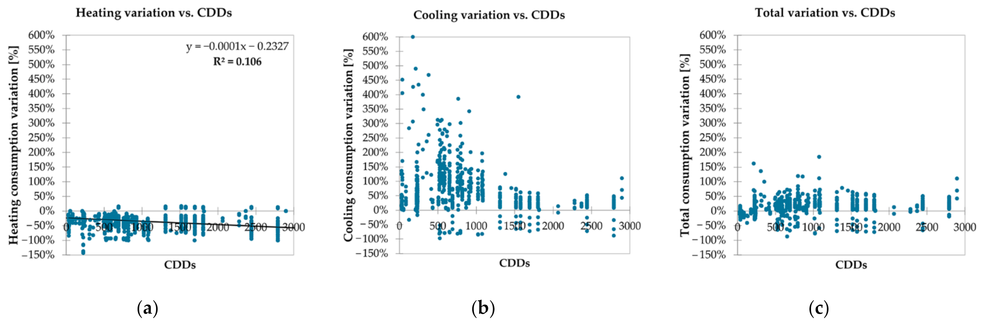
• The statistical analysis of the data collected from the reviewed manuscripts confirmed that impact analyses on the building energy consumptions lead to extremely disparate results, with a high level of heterogeneity that does not allow us to identify a synthetic combined effect. This variability depends on the climate zone, the building typology, and the methodology adopted. The attempt to find a relationship between the energy consumption variation and HDDs, CDDs, reference period, CO2 concentration, did not result in the identification of strong correlations between the parameters. Thereby, two moderate linear correlations were identified. The former was found between the heating consumption variation and HDDs, which appear to be linked by a moderate positive linear correlation, because, as HDDs increase, there is a lower reduction in heating consumptions. The latter was found between the total consumption and HDDs. Indeed, the increase in total consumption is higher in areas characterized by smaller values of HDDs, decreasing progressively as the HDDs increase, until reaching negative values.

References

- IPCC. Summary for Policymakers. In Climate Change 2021: The Physical Science Basis. Contribution of Working Group I to the Sixth Assessment Report of the Intergovernmental Panel on Climate Change; Masson-Delmotte, V., Zhai, P., Pirani, A., Connors, S.L., Péan, C., Berger, S., Caud, N., Chen, Y., Goldfarb, L., Gomis, M.I., et al., Eds.; Cambridge University Press: Cambridge, UK, 2021; in press. [Google Scholar]
- IPCC. Climate Change 2014: Mitigation of Climate Change. Contribution of Working Group III to the Fifth Assessment Report of the Intergovernmental Panel on Climate Change; Edenhofer, O., Sokona, Y., Minx, J.C., Farahani, E., Kadner, S., Seyboth, K., Adler, A., Baum, I., Brunner, S., Kriemann, B., et al., Eds.; Cambridge University Press: Cambridge, UK; New York, NY, USA, 2014. [Google Scholar]
- IEA; UNEP. 2019 Global Status Report for Buildings and Construction: Towards a Zero-Emissions, Efficient and Resilient Buildings and Constructi on Sector; UNEP: Nairobi, Kenya, 2019; Volume 224, ISBN 9789280737684. [Google Scholar]
- Bungău, C.C.; Prada, I.F.; Prada, M.; Bungău, C. Design and Operation of Constructions: A Healthy Living Environment-Parametric Studies and New Solutions. Sustainability 2019, 11, 6824. [Google Scholar] [CrossRef] [Green Version]
- Mostafavi, F.; Tahsildoost, M.; Zomorodian, Z.S. Energy efficiency and carbon emission in high-rise buildings: A review (2005–2020). Build. Environ. 2021, 206, 108329. [Google Scholar] [CrossRef]
- Fernandes, J.; Santos, M.C.; Castro, R. Introductory Review of Energy Efficiency in Buildings Retrofits. Energies 2021, 14, 8100. [Google Scholar] [CrossRef]
- Prada, M.; Prada, I.F.; Cristea, M.; Popescu, D.E.; Bungău, C.; Aleya, L.; Bungău, C.C. New solutions to reduce greenhouse gas emissions through energy efficiency of buildings of special importance—Hospitals. Sci. Total Environ. 2020, 718, 137446. [Google Scholar] [CrossRef]
- Revi, A.; Satterthwaite, D.; Aragón-Durand, F.; Corfee-Morlot, J.; Kiunsi, R.B.R.; Pelling, M.; Roberts, D.C.; Solecki, W. 2014: Urban areas. In Climate Change 2014: Impacts, Adaptation, and Vulnerability. Part A: Global and Sectoral Aspects. Contribution of Working Group II to the Fifth Assessment Report of the Intergovernmental Panel on Climate Change; Field, C.B.V.R., Barros, D.J., Dokken, K.J., Mach, M.D., Mastrandrea, T.E., Bilir, M., Chatterjee, K.L., Ebi, Y.O., Estrada, R.C., Genova, B., et al., Eds.; Cambridge University Press: Cambridge, UK; New York, NY, USA, 2014; pp. 535–612. [Google Scholar]
- Moazami, A.; Nik, V.M.; Carlucci, S.; Geving, S. Impacts of future weather data typology on building energy performance—Investigating long-term patterns of climate change and extreme weather conditions. Appl. Energy 2019, 238, 696–720. [Google Scholar] [CrossRef]
- Yang, L.; Yan, H.; Lam, J.C. Thermal comfort and building energy consumption implications—A review. Appl. Energy 2014, 115, 164–173. [Google Scholar] [CrossRef]
- Picard, T.; Hong, T.; Luo, N.; Lee, S.H.; Sun, K. Robustness of energy performance of Zero-Net-Energy (ZNE) homes. Energy Build. 2020, 224, 110251. [Google Scholar] [CrossRef]
- United Nations Framework Convention on Climate Change (UNFCCC). Paris Agreement; United Nations: Paris, France, 2015; pp. 1–27. [Google Scholar]
- IPCC. Global Warming of 1.5 °C: An IPCC Special Report on the Impacts of Global Warming of 1.5 °C above Pre-Industrial Levels and Related Global Greenhouse Gas Emission Pathways, in the Context of Strengthening the Global Response to the Threat of Climate Change, Sustainable Development, and Efforts to Eradicate Poverty; Masson-Delmotte, V., Zhai, P., Pörtner, H.-O., Roberts, D., Skea, J., Shukla, P.R., Pirani, A., Moufouma-Okia, W., Péan, C., Pidcock, R., et al., Eds.; IPCC: Geneva, Switzerland, 2018. [Google Scholar]
- Stagrum, A.E.; Andenæs, E.; Kvande, T.; Lohne, J. Climate change adaptation measures for buildings—A scoping review. Sustainability 2020, 12, 1721. [Google Scholar] [CrossRef] [Green Version]
- Scott, M.J.; Wrench, L.E.; Hadley, D.L. Effects of climate change on commercial building energy demand. Energy Sources 1994, 16, 317–332. [Google Scholar] [CrossRef]
- Rosenthal, D.H.; Gruenspecht, H.K.; Moran, E.A. Effects of global warming on energy use for space heating and cooling in the United States. Energy J. 1995, 16. [Google Scholar] [CrossRef]
- Nguyen, A.T.; Rockwood, D.; Doan, M.K.; Dung Le, T.K. Performance assessment of contemporary energy-optimized office buildings under the impact of climate change. J. Build. Eng. 2021, 35, 102089. [Google Scholar] [CrossRef]
- Zhai, Z.J.; Helman, J.M. Implications of climate changes to building energy and design. Sustain. Cities Soc. 2019, 44, 511–519. [Google Scholar] [CrossRef]
- Yassaghi, H.; Hoque, S. An Overview of Climate Change and Building Energy: Performance, Responses and Uncertainties. Buildings 2019, 9, 166. [Google Scholar] [CrossRef] [Green Version]
- Ciancio, V.; Salata, F.; Falasca, S.; Curci, G.; Golasi, I.; de Wilde, P. Energy demands of buildings in the framework of climate change: An investigation across Europe. Sustain. Cities Soc. 2020, 60, 102213. [Google Scholar] [CrossRef]
- Pérez-Lombard, L.; Ortiz, J.; Pout, C. A review on buildings energy consumption information. Energy Build. 2008, 40, 394–398. [Google Scholar] [CrossRef]
- Herrera, M.; Natarajan, S.; Coley, D.A.; Kershaw, T.; Ramallo-González, A.P.; Eames, M.; Fosas, D.; Wood, M. A review of current and future weather data for building simulation. Build. Serv. Eng. Res. Technol. 2017, 38, 602–627. [Google Scholar] [CrossRef] [Green Version]
- Nakicenovic, N.; Alcamo, J.; Grubler, A.; Riahi, K.; Roehrl, R.; Rogner, H.-H.; Victor, N. Special Report on Emissions Scenarios (SRES), a Special Report of Working Group III of the Intergovernmental Panel on Climate Change; Cambridge University Press: Cambridge, UK, 2000. [Google Scholar]
- IPCC. Climate Change 2014: Synthesis Report. In Contribution of Working Groups I, II and III to the Fifth Assessment Report of the Intergovernmental Panel on Climate Change; Core Writing Team, Pachauri, R.K., Meyer, L.A., Eds.; IPCC: Geneva, Switzerland, 2014; p. 151. [Google Scholar]
- Cellura, M.; Guarino, F.; Longo, S.; Tumminia, G. Climate change and the building sector: Modelling and energy implications to an office building in southern Europe. Energy Sustain. Dev. 2018, 45, 46–65. [Google Scholar] [CrossRef]
- Guan, L. Preparation of future weather data to study the impact of climate change on buildings. Build. Environ. 2009, 44, 793–800. [Google Scholar] [CrossRef]
- Nik, V.M. Making energy simulation easier for future climate—Synthesizing typical and extreme weather data sets out of regional climate models (RCMs). Appl. Energy 2016, 177, 204–226. [Google Scholar] [CrossRef]
- Kirtman, B.; Power, S.B.; Adedoyin, J.A.; Boer, G.J.; Bojariu, R.; Camilloni, I.; Doblas-Reyes, F.J.; Fiore, A.M.; Kimoto, M.; Meehl, G.A.; et al. Near-term Climate Change: Projections and Predictability. In Climate Change 2013: The Physical Science Basis. Contribution of Working Group I to the Fifth Assessment Report of the Intergovernmental Panel on Climate Change; Stocker, T.F., Qin, D., Plattner, G.-K., Tignor, M., Allen, S.K., Boschung, J., Nauels, A., Xia, Y., Bex, V., Midgley, P.M., Eds.; Cambridge University Press: Cambridge, UK; New York, NY, USA, 2013. [Google Scholar]
- Ismail, F.H.; Shahrestani, M.; Vahdati, M.; Boyd, P.; Donyavi, S. Climate change and the energy performance of buildings in the future—A case study for prefabricated buildings in the UK. J. Build. Eng. 2021, 39, 102285. [Google Scholar] [CrossRef]
- Flato, G.; Marotzke, J.; Abiodun, B.; Braconnot, P.; Chou, S.C.; Collins, W.; Cox, P.; Driouech, F.; Emori, S.; Eyring, V.; et al. Evaluation of Climate Models. In Climate Change 2013: The Physical Science Basis. Contribution of Working Group I to the Fifth Assessment Report of the Intergovernmental Panel on Climate Change; Stocker, T.F., Qin, D., Plattner, G.-K., Tignor, M., Allen, S.K., Boschung, J., Nauels, A., Xia, Y., Bex, V., Midgley, P.M., Eds.; Cambridge University Press: Cambridge, UK; New York, NY, USA, 2013. [Google Scholar]
- Uppala, S.M.; Kallberg, P.W.; Simmons, A.J.; Andrae, U.; Bechtold, V.D.; Fiorino, M.; Gibson, J.K.; Haseler, J.; Hernandez, A.; Kelly, G.A.; et al. The ERA-40 re-analysis. Q. J. R. Meteorol. Soc. 2005, 131, 2961–3012. [Google Scholar] [CrossRef]
- Belcher, S.E.; Hacker, J.N.; Powell, D.S. Constructing design weather data for future climates. Build. Serv. Eng. Res. Technol. 2005, 26, 49–61. [Google Scholar] [CrossRef]
- Van Paassen, A.H.C.; Luo, Q. Weather data generator to study climate change on buildings. Build. Serv. Eng. Res. Technol. Int. J. 2002, 23, 251–258. [Google Scholar] [CrossRef]
- Adelard, L.; Boyer, H.; Garde, F.G.J. Detailed weather data generator for building simulations. Energy Build. 2000, 31, 75–88. [Google Scholar] [CrossRef] [Green Version]
- Berardi, U.; Jafarpur, P. Assessing the impact of climate change on building heating and cooling energy demand in Canada. Renew. Sustain. Energy Rev. 2020, 121, 109681. [Google Scholar] [CrossRef]
- Robert, A.; Kummert, M. Designing net-zero energy buildings for the future climate, not for the past. Build. Environ. 2012, 55, 150–158. [Google Scholar] [CrossRef]
- Trzaska, S.; Schnarr, E. A Review of Downscaling Methods for Climate Change Projections; United States Agency for International Development: Washington, DC, USA, 2014; pp. 1–43. [Google Scholar]
- Amato, A.D.; Ruth, M.; Kirshen, P.; Horwitz, J. Regional energy demand responses to climate change: Methodology and application to the commonwealth of massachusetts. Clim. Change 2005, 71, 175–201. [Google Scholar] [CrossRef]
- Wang, H.; Chen, Q. Impact of climate change heating and cooling energy use in buildings in the United States. Energy Build. 2014, 82, 428–436. [Google Scholar] [CrossRef] [Green Version]
- Santamouris, M.; Vasilakopoulou, K. Present and future energy consumption of buildings: Challenges and opportunities towards decarbonisation. e-Prime Adv. Electr. Eng. Electron. Energy 2021, 1, 100002. [Google Scholar] [CrossRef]
- Guan, L. Implication of global warming on air-conditioned office buildings in Australia. Build. Res. Inf. 2009, 37, 43–54. [Google Scholar] [CrossRef] [Green Version]
- Li, Y.; Wang, W.; Wang, Y.; Xin, Y.; He, T.; Zhao, G. A Review of Studies Involving the Effects of Climate Change on the Energy Consumption for Building Heating and Cooling. Int. J. Environ. Res. Public Health 2021, 18, 40. [Google Scholar] [CrossRef]
- Li, D.H.W.; Yang, L.; Lam, J.C. Impact of climate change on energy use in the built environment in different climate zones—A review. Energy 2012, 42, 103–112. [Google Scholar] [CrossRef]
- Page, M.J.; Mckenzie, J.E.; Bossuyt, P.M.; Boutron, I.; Hoffmann, T.C.; Mulrow, C.D.; Shamseer, L.; Tetzlaff, J.M.; Akl, E.A.; Brennan, S.E.; et al. The PRISMA 2020 statement: An updated guideline for reporting systematic reviews. BMJ 2021, 372, n71. [Google Scholar] [CrossRef]
- Zhu, J.; Liu, W. A tale of two databases: The use of Web of Science and Scopus in academic papers. Scientometrics 2020, 123, 321–335. [Google Scholar] [CrossRef] [Green Version]
- Aghaei Chadegani, A.; Salehi, H.; Yunus, M.; Farhadi, H.; Fooladi, M.; Farhadi, M.; Ale Ebrahim, N. A Comparison between Two Main Academic Literature Collections: Web of Science and Scopus Databases. Asian Soc. Sci. 2013, 9, 18–26. [Google Scholar] [CrossRef] [Green Version]
- Mongeon, P.; Paul-Hus, A. The Journal Coverage of Web of Science and Scopus: A Comparative Analysis. Scientometrics 2015, 106, 213–228. [Google Scholar] [CrossRef]
- Zhao, X.; Zuo, J.; Wu, G.; Huang, C. A bibliometric review of green building research 2000–2016. Archit. Sci. Rev. 2019, 62, 74–88. [Google Scholar] [CrossRef]
- Peel, M.C.; Finlayson, B.L.; McMahon, T.A. Updated world map of the Köppen-Geiger climate classification. Hydrol. Earth Syst. Sci. 2007, 11, 1633–1644. [Google Scholar] [CrossRef] [Green Version]
- U.S. Department of Energy’s (DOE). Energy Plus Weather Data. Available online: https://energyplus.net/weather (accessed on 30 September 2021).
- Meteotest Meteonorm Global Meteorological Database. Available online: https://www.energiehaus.es/wp-content/uploads/2015/06/flyer-meteonorm-7.pdf (accessed on 30 September 2021).
- IPCC. Climate Change 2001: The Scientific Basis. Contribution of Working Group I to the Third Assessment Report of the Intergovernmental Panel on Climate Change; Houghton, J.T., Ding, Y., Griggs, D.J., Noguer, M., van der Linden, P.J., Dai, X., Maskell, K., Johnson, C.A., Eds.; Cambridge University Press: Cambridge, UK; New York, NY, USA, 2001; p. 881. [Google Scholar]
- Meinshausen, M.; Nicholls, Z.R.J.; Lewis, J.; Gidden, M.J.; Vogel, E.; Freund, M.; Beyerle, U.; Gessner, C.; Nauels, A.; Bauer, N.; et al. The shared socio-economic pathway (SSP) greenhouse gas concentrations and their extensions to 2500. Geosci. Model Dev. 2020, 13, 3571–3605. [Google Scholar] [CrossRef]
- OriginLab Corporation Origin. Available online: https://www.originlab.com (accessed on 30 July 2021).
- Borenstein, M.; Hedges, L.V.; Higgins, J.P.T.; Rothstein, H.R. Introductionto Meta-Analysis; John Wiley & Sons: Chichester, UK, 2009. [Google Scholar]
- Higgins, J.P.T.; Thompson, S.G.; Deeks, J.J.; Altman, D.G. Measuring inconsistency in meta-analyses. BMJ 2003, 327, 557–560. [Google Scholar] [CrossRef] [Green Version]
- Lionello, P.; Scarascia, L. The relation between climate change in the Mediterranean region and global warming. Reg. Environ. Chang. 2018, 18, 1481–1493. [Google Scholar] [CrossRef]
- Huang, J.; Gurney, K.R. The variation of climate change impact on building energy consumption to building type and spatiotemporal scale. Energy 2016, 111, 137–153. [Google Scholar] [CrossRef] [Green Version]
- Zheng, Y.; Weng, Q. Modeling the effect of climate change on building energy demand in Los Angeles county by using a GIS-based high spatial- and temporal-resolution approach. Energy 2019, 176, 641–655. [Google Scholar] [CrossRef]
- Li, M.; Cao, J.; Xiong, M.; Li, J.; Feng, X.; Meng, F. Different responses of cooling energy consumption in office buildings to climatic change in major climate zones of China. Energy Build. 2018, 173, 38–44. [Google Scholar] [CrossRef]
- Nematchoua, M.K.; Yvon, A.; Kalameu, O.; Asadi, S.; Choudhary, R.; Reiter, S. Impact of climate change on demands for heating and cooling energy in hospitals: An in-depth case study of six islands located in the Indian Ocean region. Sustain. Cities Soc. 2019, 44, 629–645. [Google Scholar] [CrossRef]
- Sajjadian, S.M. Performance evaluation ofwell-insulated versions of contemporary wall systems-a case study of london for a warmer climate. Buildings 2017, 7, 6. [Google Scholar] [CrossRef] [Green Version]
- Shen, P. Impacts of climate change on U. S. building energy use by using downscaled hourly future weather data. Energy Build. 2017, 134, 61–70. [Google Scholar] [CrossRef]
- Dodoo, A.; Gustavsson, L. Energy use and overheating risk of Swedish multi-storey residential buildings under different climate scenarios. Energy 2016, 97, 534–548. [Google Scholar] [CrossRef]
- Liu, S.; Kwok, Y.T.; Lau, K.K.L.; Tong, H.W.; Chan, P.W.; Edward, N.G. Development and application of future design weather data for evaluating the building thermal-energy performance in subtropical Hong Kong. Energy Build. 2020, 209, 109696. [Google Scholar] [CrossRef]
- Suárez, R.; Escandón, R.; López-Pérez, R.; León-Rodríguez, Á.L.; Klein, T.; Silvester, S. Impact of climate change: Environmental assessment of passive solutions in a single-family home in Southern Spain. Sustainability 2018, 10, 2914. [Google Scholar] [CrossRef] [Green Version]
- Daly, D.; Cooper, P.; Ma, Z. Implications of global warming for commercial building retrofitting in Australian cities. Build. Environ. 2014, 74, 86–95. [Google Scholar] [CrossRef]
- Soutullo, S.; Giancola, E.; Jiménez, M.J.; Ferrer, J.A.; Sánchez, M.N. How climate trends impact on the thermal performance of a typical residential building in Madrid. Energies 2020, 13, 237. [Google Scholar] [CrossRef] [Green Version]
- Pérez-Andreu, V.; Aparicio-Fernández, C.; Martínez-Ibernón, A.; Vivancos, J.L. Impact of climate change on heating and cooling energy demand in a residential building in a Mediterranean climate. Energy 2018, 165, 63–74. [Google Scholar] [CrossRef]
- Hasan, A.; Bahadori-Jahromi, A.; Mylona, A.; Ferri, M.; Tahayori, H. Investigating the potential impact of future climate change on uk supermarket building performance. Sustainability 2021, 13, 33. [Google Scholar] [CrossRef]
- Cox, R.A.; Drews, M.; Rode, C.; Nielsen, S.B. Simple future weather files for estimating heating and cooling demand. Build. Environ. 2015, 83, 104–114. [Google Scholar] [CrossRef] [Green Version]
- Berger, T.; Amann, C.; Formayer, H.; Korjenic, A.; Pospichal, B.; Neururer, C.; Smutny, R. Impacts of urban location and climate change upon energy demand of office buildings in Vienna, Austria. Build. Environ. 2014, 81, 258–269. [Google Scholar] [CrossRef]
- Sustainable Energy Research Group Climate Change World Weather File Generator for Worldwide Weather Data. Available online: http://www.energy.soton.ac.uk/ccworldweathergen (accessed on 15 November 2021).
- WeatherShift. Available online: www.weathershift.com (accessed on 15 November 2021).
- Chakraborty, D.; Alam, A.; Chaudhuri, S.; Başağaoğlu, H.; Sulbaran, T.; Langar, S. Scenario-based prediction of climate change impacts on building cooling energy consumption with explainable artificial intelligence. Appl. Energy 2021, 291, 116807. [Google Scholar] [CrossRef]
- Dolinar, M.; Vidrih, B.; Kajfež-Bogataj, L.; Medved, S. Predicted changes in energy demands for heating and cooling due to climate change. Phys. Chem. Earth 2010, 35, 100–106. [Google Scholar] [CrossRef]
- Radhi, H. Evaluating the potential impact of global warming on the UAE residential buildings—A contribution to reduce the CO2 emissions. Build. Environ. 2009, 44, 2451–2462. [Google Scholar] [CrossRef]
- Nurlybekova, G.; Memon, S.A.; Adilkhanova, I. Quantitative evaluation of the thermal and energy performance of the PCM integrated building in the subtropical climate zone for current and future climate scenario. Energy 2021, 219, 119587. [Google Scholar] [CrossRef]
- Ptootkaboni, M.; Ballarini, I.; Zinzi, M.; Corrado, V. A comparative analysis of different future weather data for building energy performance simulation. Climate 2021, 9, 37. [Google Scholar] [CrossRef]
- Li, M.; Guo, J.; Tian, Z.; Shi, J.; Xiong, M.; Xiang, C. Future climate change and building energy demand in Tianjin, China. Build. Serv. Eng. Res. Technol. 2014, 35, 362–375. [Google Scholar] [CrossRef]
- Xiang, C.; Tian, Z. Impact of climate change on building heating energy consumption in Tianjin. Front. Energy 2013, 7, 518–524. [Google Scholar] [CrossRef]
- Wan, K.K.W.; Li, D.H.W.; Pan, W.; Lam, J.C. Impact of climate change on building energy use in different climate zones and mitigation and adaptation implications. Appl. Energy 2012, 97, 274–282. [Google Scholar] [CrossRef]
- Wan, K.K.W.; Li, D.H.W.; Lam, J.C. Assessment of climate change impact on building energy use and mitigation measures in subtropical climates. Energy 2011, 36, 1404–1414. [Google Scholar] [CrossRef]
- Hosseini, M.; Bigtashi, A.; Lee, B. Generating future weather files under climate change scenarios to support building energy simulation—A machine learning approach. Energy Build. 2021, 230, 110543. [Google Scholar] [CrossRef]
- Marion, W.; Urban, K. User’s Manual for TMY2s (Typical Meteorological Years)—Derived from the 1961–1990 National Solar Radiation Data Base; National Renewable Energy Laboratory: Golden, CO, USA, 1995. [Google Scholar]
- Wilcox, S.; Marion, W. Users Manual for TMY3 Data Sets; National Renewable Energy Laboratory: Golden, CO, USA, 2008. [Google Scholar]
- Thevenard, D.J.; Brunger, A.P. The development of typical weather years for international locations: Part I, Algorithms. ASHRAE Trans. 2002, 108, 376–383. [Google Scholar]
- Papakostas, K.; Mavromatis, T.; Kyriakis, N. Impact of the ambient temperature rise on the energy consumption for heating and cooling in residential buildings of Greece. Renew. Energy 2010, 35, 1376–1379. [Google Scholar] [CrossRef]
- Filippín, C.; Ricard, F.; Flores Larsen, S.; Santamouris, M. Retrospective analysis of the energy consumption of single-family dwellings in central Argentina. Retrofitting and adaptation to the climate change. Renew. Energy 2017, 101, 1226–1241. [Google Scholar] [CrossRef]
- Arima, Y.; Ooka, R.; Kikumoto, H.; Yamanaka, T. Effect of climate change on building cooling loads in Tokyo in the summers of the 2030s using dynamically downscaled GCM data. Energy Build. 2016, 114, 123–129. [Google Scholar] [CrossRef]
- Kikumoto, H.; Ooka, R.; Arima, Y.; Yamanaka, T. Study on the future weather data considering the global and local climate change for building energy simulation. Sustain. Cities Soc. 2015, 14, 404–413. [Google Scholar] [CrossRef]
- Central Limit Theorem. The Concise Encyclopedia of Statistics; Springer: New York, NY, USA, 2008; pp. 66–68. ISBN 978-0-387-32833-1. [Google Scholar]
- Altman, D.; Bland, J. Statistics notes: The normal distribution. BMJ 1995, 310, 298. [Google Scholar] [CrossRef] [Green Version]
- Addinsoft. XLSTAT: Data Analysis and Statistical Solution for Microsoft Excel 2021. Long Island, NY, USA. Available online: https://www.xlstat.com (accessed on 15 November 2021).
- Croux, C.; Dehon, C. Influence functions of the Spearman and Kendall correlation measures. Stat. Methods Appl. 2010, 19, 497–515. [Google Scholar] [CrossRef] [Green Version]
- IEA. World Energy Outlook 2021; IEA: Paris, France, 2021. [Google Scholar]
- Santamouris, M.; Cartalis, C.; Synnefa, A.; Kolokotsa, D. On the impact of urban heat island and global warming on the power demand and electricity consumption of buildings—A review. Energy Build. 2015, 98, 119–124. [Google Scholar] [CrossRef]
- Santamouris, M. Cooling the buildings—past, present and future. Energy Build. 2016, 128, 617–638. [Google Scholar] [CrossRef]
- Santamouris, M. Present and Future Challenges and Opportunities in the Built Environment. In Bioclimatic Approaches in Urban and Building Design; Springer: Cham, Switzerland, 2021. [Google Scholar] [CrossRef]
- Mikolajewicz, N.; Komarova, S.V. Meta-Analytic Methodology for Basic Research: A Practical Guide. Front. Physiol. 2019, 10, 203. [Google Scholar] [CrossRef]
- Prignon, M.; Altomonte, S.; Ossio, F.; Dawans, A.; Van Moeseke, G. On the applicability of meta-analysis to evaluate airtightness performance of building components. Build. Environ. 2021, 194, 107684. [Google Scholar] [CrossRef]
- Bamdad, K.; Cholette, M.E.; Omrani, S.; Bell, J. Future energy-optimised buildings—Addressing the impact of climate change on buildings. Energy Build. 2021, 231, 110610. [Google Scholar] [CrossRef]
- Rodríguez, M.V.; Cordero, A.S.; Melgar, S.G.; Andújar Márquez, J.M. Impact of global warming in subtropical climate buildings: Future trends and mitigation strategies. Energies 2020, 13, 6188. [Google Scholar] [CrossRef]
- Fabbri, K.; Gaspari, J.; Felicioni, L. Climate change effect on building performance: A case study in New York. Energies 2020, 13, 3160. [Google Scholar] [CrossRef]
- Fathi, S.; Srinivasan, R.S.; Kibert, C.J.; Steiner, R.L.; Demirezen, E. AI-based campus energy use prediction for assessing the effects of climate change. Sustainability 2020, 12, 3223. [Google Scholar] [CrossRef] [Green Version]
- Mangan, S.D.; Koçlar Oral, G. Impacts of future weather data on the energy performance of buildings in the context of urban geometry. Cogent Eng. 2020, 7, 1714112. [Google Scholar] [CrossRef]
- Rouault, F.; Ossio, F.; González-Levín, P.; Meza, F. Impact of Climate Change on the Energy Needs of Houses in Chile. Sustainability 2019, 11, 7068. [Google Scholar] [CrossRef] [Green Version]
- Dodoo, A.; Ayarkwa, J. Effects of climate change for thermal comfort and energy performance of residential buildings in a Sub-Saharan African climate. Buildings 2019, 9, 215. [Google Scholar] [CrossRef] [Green Version]
- Dino, I.G.; Meral Akgül, C. Impact of climate change on the existing residential building stock in Turkey: An analysis on energy use, greenhouse gas emissions and occupant comfort. Renew. Energy 2019, 141, 828–846. [Google Scholar] [CrossRef]
- Flores-Larsen, S.; Filippín, C.; Barea, G. Impact of climate change on energy use and bioclimatic design of residential buildings in the 21st century in Argentina. Energy Build. 2019, 184, 216–229. [Google Scholar] [CrossRef]
- Jiang, A.; Zhu, Y.; Elsafty, A.; Tumeo, M. Effects of Global Climate Change on Building Energy Consumption and Its Implications in Florida. Int. J. Constr. Educ. Res. 2018, 14, 22–45. [Google Scholar] [CrossRef]
- Jylhä, K.; Jokisalo, J.; Ruosteenoja, K.; Pilli-Sihvola, K.; Kalamees, T.; Seitola, T.; Mäkelä, H.M.; Hyvönen, R.; Laapas, M.; Drebs, A. Energy demand for the heating and cooling of residential houses in Finland in a changing climate. Energy Build. 2015, 99, 104–116. [Google Scholar] [CrossRef]
- Pierangioli, L.; Cellai, G.; Ferrise, R.; Trombi, G.; Bindi, M. Effectiveness of passive measures against climate change: Case studies in Central Italy. Build. Simul. 2017, 10, 459–479. [Google Scholar] [CrossRef]
- Hosseini, M.; Tardy, F.; Lee, B. Cooling and heating energy performance of a building with a variety of roof designs; the effects of future weather data in a cold climate. J. Build. Eng. 2018, 17, 107–114. [Google Scholar] [CrossRef] [Green Version]
- Invidiata, A.; Ghisi, E. Impact of climate change on heating and cooling energy demand in houses in Brazil. Energy Build. 2016, 130, 20–32. [Google Scholar] [CrossRef]
- Spandagos, C.; Ng, T.L. Equivalent full-load hours for assessing climate change impact on building cooling and heating energy consumption in large Asian cities. Appl. Energy 2017, 189, 352–368. [Google Scholar] [CrossRef]
- Lim, J.H.; Yun, G.Y. Cooling energy implications of occupant factor in buildings under climate change. Sustainability 2017, 9, 2039. [Google Scholar] [CrossRef] [Green Version]
- Sabunas, A.; Kanapickas, A. Estimation of climate change impact on energy consumption in a residential building in Kaunas, Lithuania, using HEED Software. Energy Procedia 2017, 128, 92–99. [Google Scholar] [CrossRef]
- Shibuya, T.; Croxford, B. The effect of climate change on office building energy consumption in Japan. Energy Build. 2016, 117, 149–159. [Google Scholar] [CrossRef]
- Huang, K.T.; Hwang, R.L. Future trends of residential building cooling energy and passive adaptation measures to counteract climate change: The case of Taiwan. Appl. Energy 2016, 184, 1230–1240. [Google Scholar] [CrossRef]
- Khalfan, M.; Sharples, S. The present and future energy performance of the first passivhaus project in the Gulf region. Sustainability 2016, 8, 139. [Google Scholar] [CrossRef] [Green Version]
- Pagliano, L.; Carlucci, S.; Causone, F.; Moazami, A.; Cattarin, G. Energy retrofit for a climate resilient child care centre. Energy Build. 2016, 127, 1117–1132. [Google Scholar] [CrossRef]
- Dirks, J.A.; Gorrissen, W.J.; Hathaway, J.H.; Skorski, D.C.; Scott, M.J.; Pulsipher, T.C.; Huang, M.; Liu, Y.; Rice, J.S. Impacts of climate change on energy consumption and peak demand in buildings: A detailed regional approach. Energy 2015, 79, 20–32. [Google Scholar] [CrossRef] [Green Version]
- Wong, N.H.; Jusuf, S.K.; Syafii, N.I.; Li, W.H.; Tan, E. Mitigation Methods of Climate Change Impact on the Cooling Load of Public Residential Buildings in Singapore. J. Archit. Eng. 2013, 19, 147–155. [Google Scholar] [CrossRef]
- Chan, A.L.S.; Chow, T.T. Energy and economic performance of green roof system under future climatic conditions in Hong Kong. Energy Build. 2013, 64, 182–198. [Google Scholar] [CrossRef]
- Chow, D.H.C. The potential impact of climate change on heating and cooling loads for office buildings in the Yangtze River Delta. Int. J. Low-Carbon Technol. 2012, 7, 234–247. [Google Scholar] [CrossRef] [Green Version]
- Ouedraogo, B.I.; Levermore, G.J.; Parkinson, J.B. Future energy demand for public buildings in the context of climate change for Burkina Faso. Build. Environ. 2012, 49, 270–282. [Google Scholar] [CrossRef]
- Asimakopoulos, D.A.; Santamouris, M.; Farrou, I.; Laskari, M.; Saliari, M.; Zanis, G.; Giannakidis, G.; Tigas, K.; Kapsomenakis, J.; Douvis, C.; et al. Modelling the energy demand projection of the building sector in Greece in the 21st century. Energy Build. 2012, 49, 488–498. [Google Scholar] [CrossRef]
- Chan, A.L.S. Developing future hourly weather files for studying the impact of climate change on building energy performance in Hong Kong. Energy Build. 2011, 43, 2860–2868. [Google Scholar] [CrossRef]
- Ren, Z.; Chen, Z.; Wang, X. Climate change adaptation pathways for Australian residential buildings. Build. Environ. 2011, 46, 2398–2412. [Google Scholar] [CrossRef]
- Mourshed, M. The impact of the projected changes in temperature on heating and cooling requirements in buildings in Dhaka, Bangladesh. Appl. Energy 2011, 88, 3737–3746. [Google Scholar] [CrossRef] [Green Version]
- Lam, J.C.; Wan, K.K.W.; Lam, T.N.T.; Wong, S.L. An analysis of future building energy use in subtropical Hong Kong. Energy 2010, 35, 1482–1490. [Google Scholar] [CrossRef]
- Wang, X.; Chen, D.; Ren, Z. Assessment of climate change impact on residential building heating and cooling energy requirement in Australia. Build. Environ. 2010, 45, 1663–1682. [Google Scholar] [CrossRef]
- Jenkins, D.; Liu, Y.; Peacock, A.D. Climatic and internal factors affecting future UK office heating and cooling energy consumptions. Energy Build. 2008, 40, 874–881. [Google Scholar] [CrossRef]
- Frank, T. Climate change impacts on building heating and cooling energy demand in Switzerland. Energy Build. 2005, 37, 1175–1185. [Google Scholar] [CrossRef]
- Aguiar, R.; Oliveira, M.; Gonçalves, H. Climate change impacts on the thermal performance of Portuguese buildings. Results of the SIAM study. Build. Serv. Eng. Res. Technol. 2002, 23, 223–231. [Google Scholar] [CrossRef]