
Energy-Optimal Structures of HVAC System for Cleanrooms as a Function of Key Constant Parameters and External Climate


Abstract
:1. Introduction
- until now, researchers have mainly focused on case studies in pharmaceutical and semiconductor industries;
- optimal structures of the HVAC system are calculated by performing simulations for several predetermined acceptable variants and indicating the variant for which the annual energy consumption is minimal;
- there is no global approach to calculating the optimal structures of the HVAC system as a function of key constants parameters being the input data and describing the HVAC system.
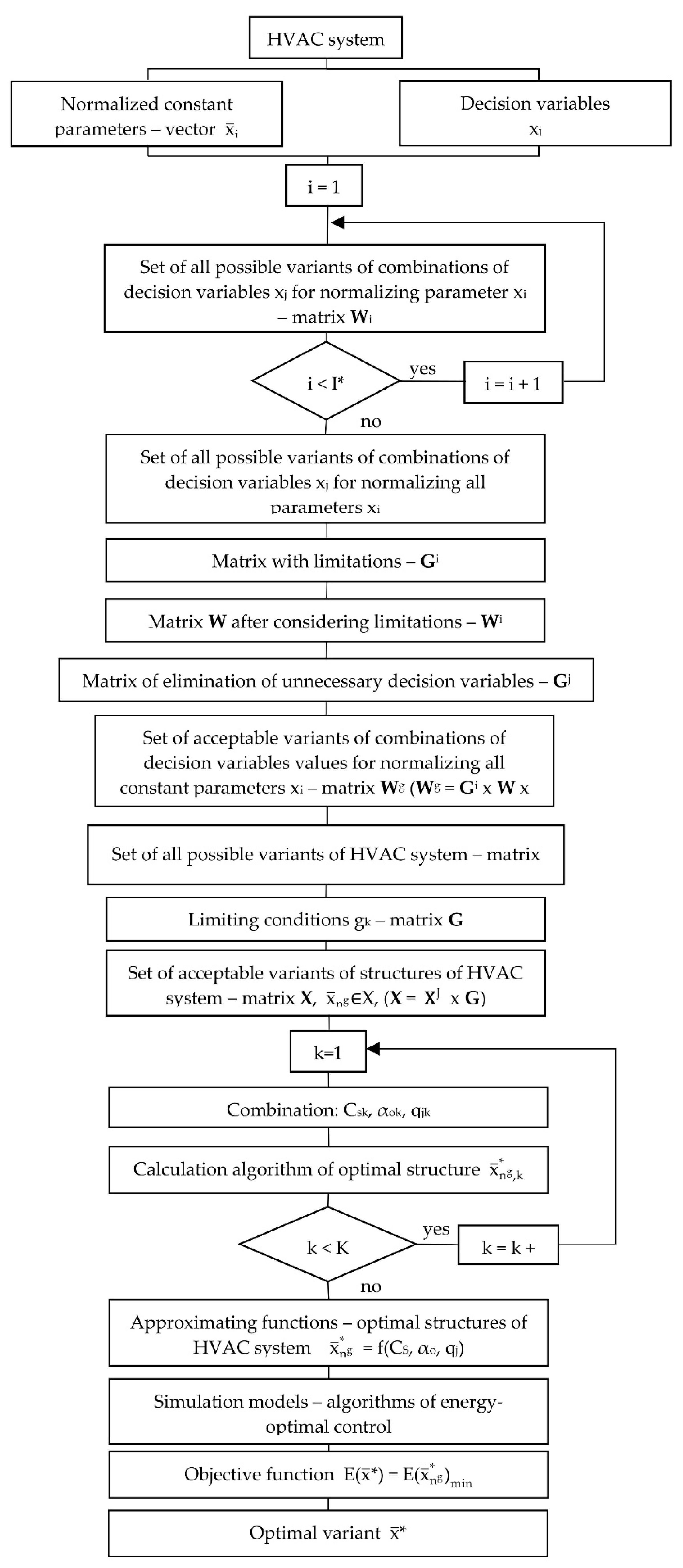
2. Research Problem, General Algorithm
- calculating the set of constant parameters and the set of decision variables xj;
- two phases of analysis: calculating the matrix of all possible variants of limiting conditions and of acceptable variants, respectively, for:
- -
- combinations of decision variables values xj for normalizing constant parameters (matrices Wi, W, Gi, Gj and Wg) and
- -
- the HVAC system (matrices XJ, G and X);
- calculating the optimal structures of HVAC systems for combinations of values of key constant parameters (arguments): cleanliness class (Csk), percentage of outdoor air (αok) and unit cooling load (qjk), k = 1…K;
- defining approximation relations = f(Csk, αok, qjk);
- defining algorithms of energy-optimal control for optimal structures of HVAC systems based on the objective function;
- calculating the optimal variant .
- determination of a set of permissible HVAC system structures—X matrix, based on the utility function (normalized constants and limiting conditions);
- determination of the optimal structure of the HVAC system— based on the key constants: Cs—cleanliness class, —unit heat load and αo—percentage of outside air;
- determination of the energy-optimal variant of the HVAC system—vector , taking into account the optimal structure and the optimal type of heat recovery.
3. Acceptable Structures of HVAC System
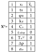
- temperature, tR
- relative humidity φR (φR1, φR2)
- acceptable concentration of contaminants, kd
- cleanliness class, CS
- overpressure, ∆p
- percentage of outdoor air, αo
- normalized constant parameters;
- a set of all possible variants of a combination of decision variables for the normalization of each individual and all constant parameters together;
- limiting conditions for variants of combinations of decision variables for the standardization of constant parameters;
- set of eliminated decision variables;
- a set of all possible variants of the HVAC system for the standardization of constant parameters;
- limiting conditions for possible variants of the HVAC system;
- set of acceptable HVAC system structures.
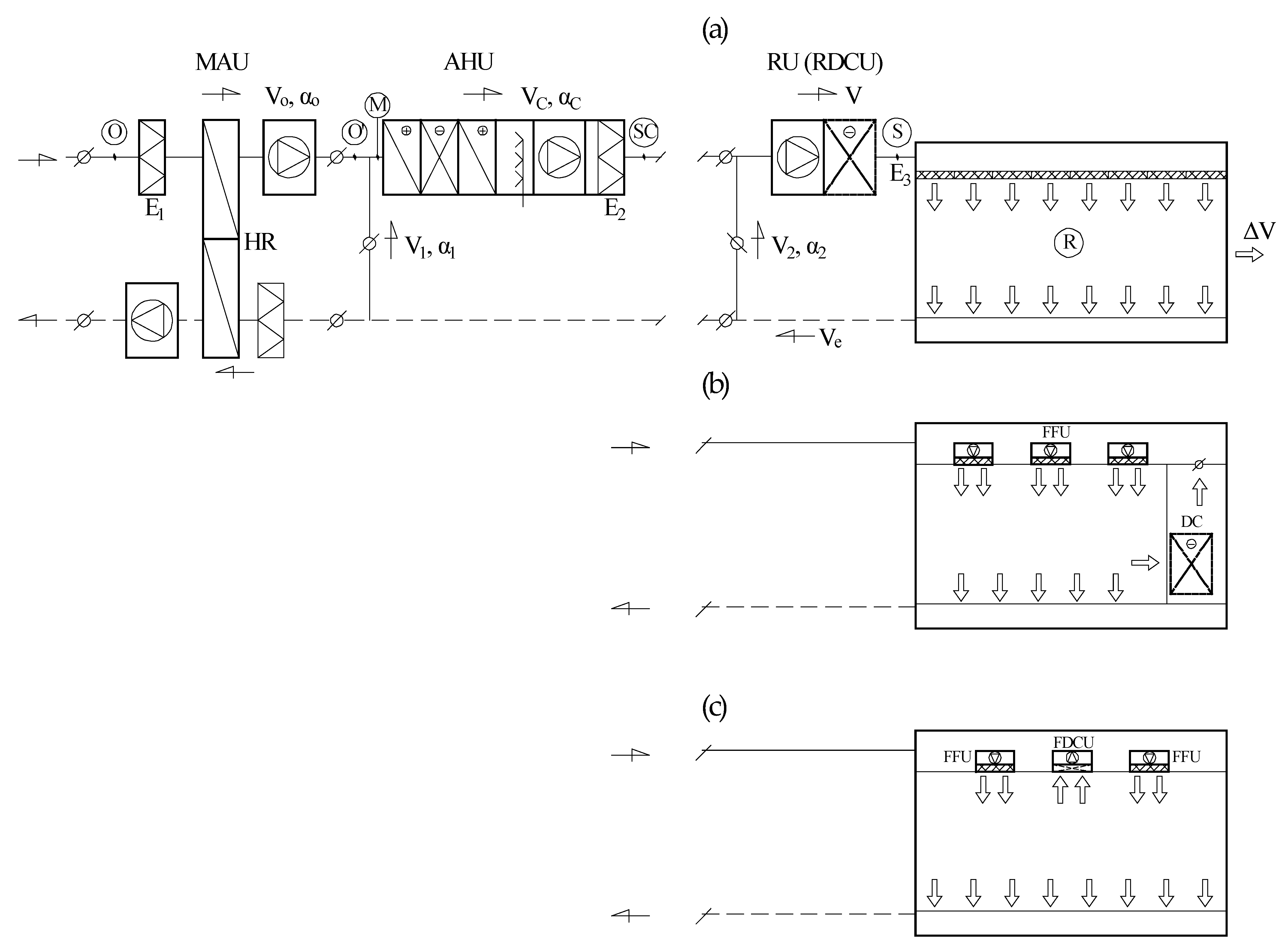
- AHU—thermodynamic treatment: heat recovery, primary heater, cooler, secondary heater and steam humidifier;
- hygienic standard: three stages of filtration, 3rd stage filter integrated with a supply diffuser, hygienic design;
- installation: variable flow regulators.
- two air handling units in cascade at the supply: MAU + AHU;
- MAU of outdoor air with heat recovery;
- AHU—thermodynamic treatment: primary heater, cooler, secondary heater and steam humidifier;
- hygienic standard: as with point b;
- installation: as with point c.
- two air handling units in cascade at the supply: AHU + RU (RDCU);
- AHU—thermodynamic treatment: heat recovery, primary heater, cooler, secondary heater and steam humidifier;
- RU (Recirculation Unit) or RDCU (Recirculation Dry Cooling Unit)—recirculation (recirculation with dry cooling);
- hygienic standard: as with point b;
- installation: as with point c.
- three air handling units in cascade at the supply: MAU + AHU + RU (RDCU);
- MAU of outdoor air with heat recovery;
- AHU—thermodynamic treatment: primary heater, cooler, secondary heater and steam humidifier;
- RU or RDCU—recirculation (recirculation with dry cooling);
- hygienic standard: as with point b;
- installation: as with point c.
4. Optimal Structures of HVAC System
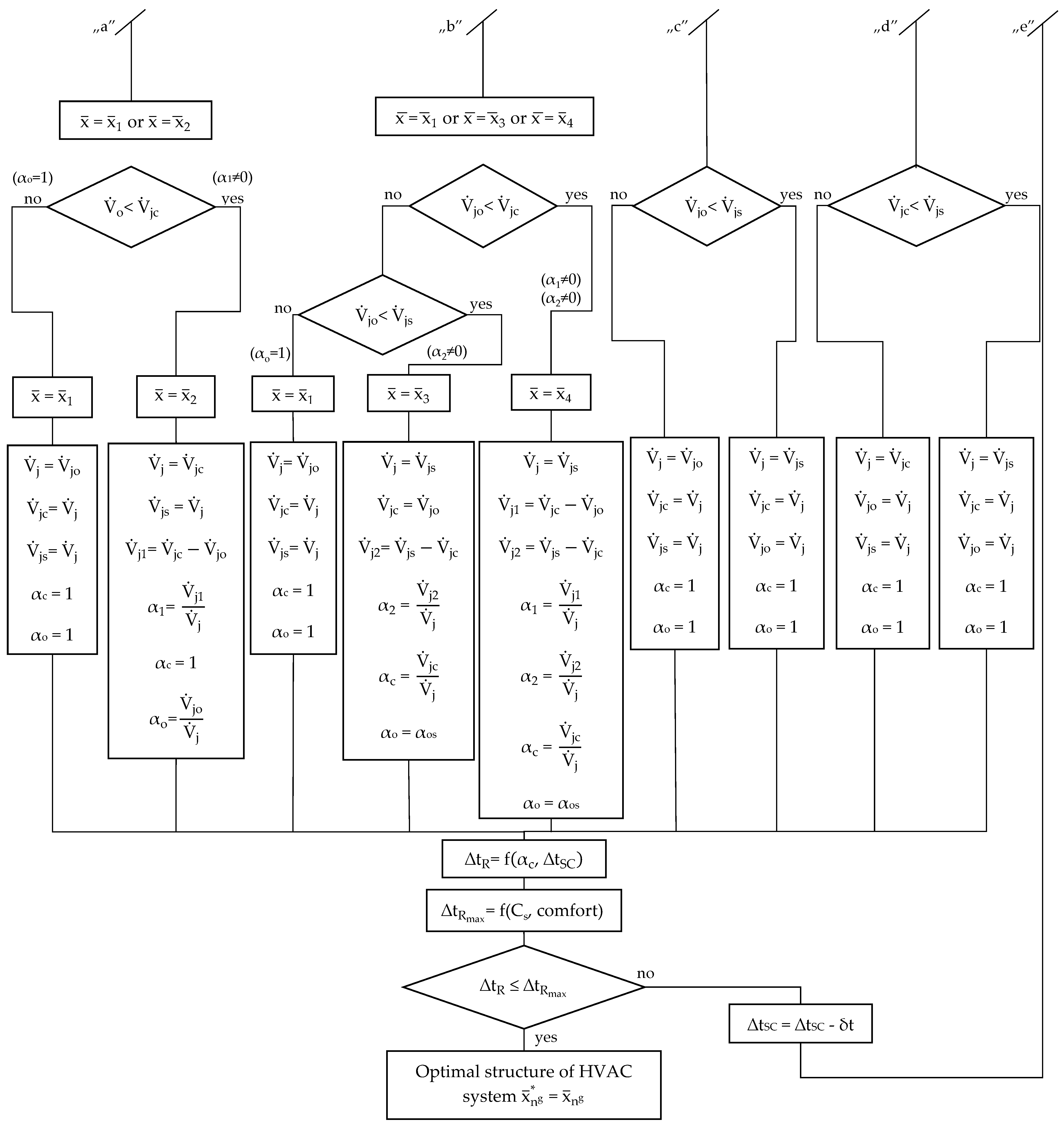
4.1. Optimal Structure Selection Algorithm
- = f(kd, ∆p, )—unit outdoor air stream as a function of hygiene requirements (the concentration of pollutants—kd), overpressure (∆p) or compensation of exhaust air from local exhausts ();
- = f(Cs)—unit air stream as a function of the room cleanliness class;
- —unit air stream as a function of the cooling loads discharged using AHU.
- qj—unit cooling loads;
- qjc—unit cooling load discharged using AHU;
- qjDC—unit cooling load discharged by dry coolers in the recirculation circuit (DCC, RDCU and RCU).
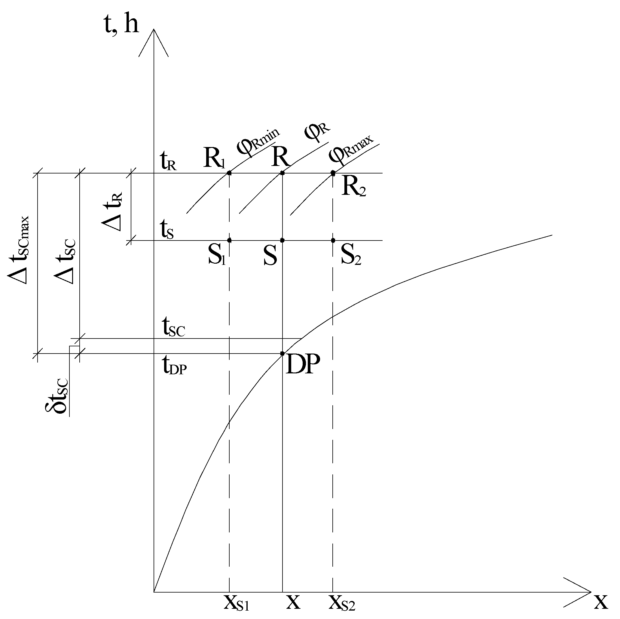
- δtSC—realistic tolerance range with temperature tSC in relation to temperature tDP, δtSC = (0 ÷ 1) °C
- tDP—dew point temperature.
- system (α1 = 0, α2 = 0, αc = 1):
- system (α1 ≠ 0, α2 = 0, αc = 1):
- system (α1 = 0, α2 ≠ 0, αc ≠ 0):
- system (α1 ≠ 0, α2 ≠ 0, αc ≠ 0):
- δt = (0.5 ÷ 1.0) °C—iterative temperature jump, and the procedure is repeated.
4.2. Optimal Structure Selection Algorithm
- dry bulb temperature changes in a narrow range of +21 ÷ +23 °C; on average, tR = +22 °C;
- relative humidity usually changes in the range of (50 ± 5)% (sometimes, the range is wider);
- the most common cleanliness classes are ISO5 classes (M3.5—cl. 100), ISO7 (M5.5—cl. 10,000) and ISO8 (M6.5—cl. 100,000) [39];
- unit cooling loads are qj = (100 ÷ 500) W/m2 [40];
- the required percentage of outdoor air is αo = (5 ÷ 100)%.
4.3. Approximating Functions
- —difference in values of the unit cooling loads in Table 3;
- ∆αog—difference of the limit value of the percentage of outdoor air in Table 3 assigned to a defined difference .
- The dominant optimal structures of HVAC system for cleanrooms with acceptable recirculation are systems with internal recirculation and systems with internal and external recirculation .
- Directional coefficients of the limit lines = aαo dividing zones of optimal structures of the HVAC system HVAC and are inversely proportional to the cleanliness classes of rooms and equal:
- a = 33.3—for ISO Class 5 (M3.5—cl.100);
- a = 8.0—for ISO Class 7 (M5.5—cl.10,000);
- a = 3.33—for ISO Class 8 (M6.5—cl.100,000),
- Systems with internal recirculation are optimal HVAC system structures for rooms with low cooling loads and relatively high percentages of outdoor air αo.
- Systems with internal and external recirculation are optimal HVAC system structures for rooms with high cooling loads and relatively low percentages of outdoor air αo.
- Systems with external recirculation are optimal HVAC system structures for rooms with high cooling loads and low requirements regarding cleanliness of high cleanliness classes.The limit line in system = f(αo) between the zone of optimal structures and or and is ordinate (horizontal line). For cleanliness classes ISO Class 8 (M6.5—cl. 100,000) the limit unit cooling load equals = 332 W/m2. For unit cooling loads , the optimal structure of the HVAC system is a system with external recirculation , while, for optimal structures are systems with internal recirculation or systems with internal and external recirculation . The limit of division of optimal zones and is line = aαo.
- Approximating functions in the form of a graph = f(CS, αo, qj) with zones of optimal structures of the HVAC system for cleanrooms in Figure 5 are of great application significance at the stage of selecting and designing energy-efficient HVAC systems of such rooms.Based on cleanliness class Cs of unit cooling loads and the percentage of outdoor air , they make it possible to unambiguously calculate an energy-optimal structure of a HVAC system for a cleanroom.For “middle” cleanliness classes between ISO5 and ISO7, zones of optimal HVAC structures can be calculated using interpolation.
5. Heat Recovery, Energy-Optimal Control
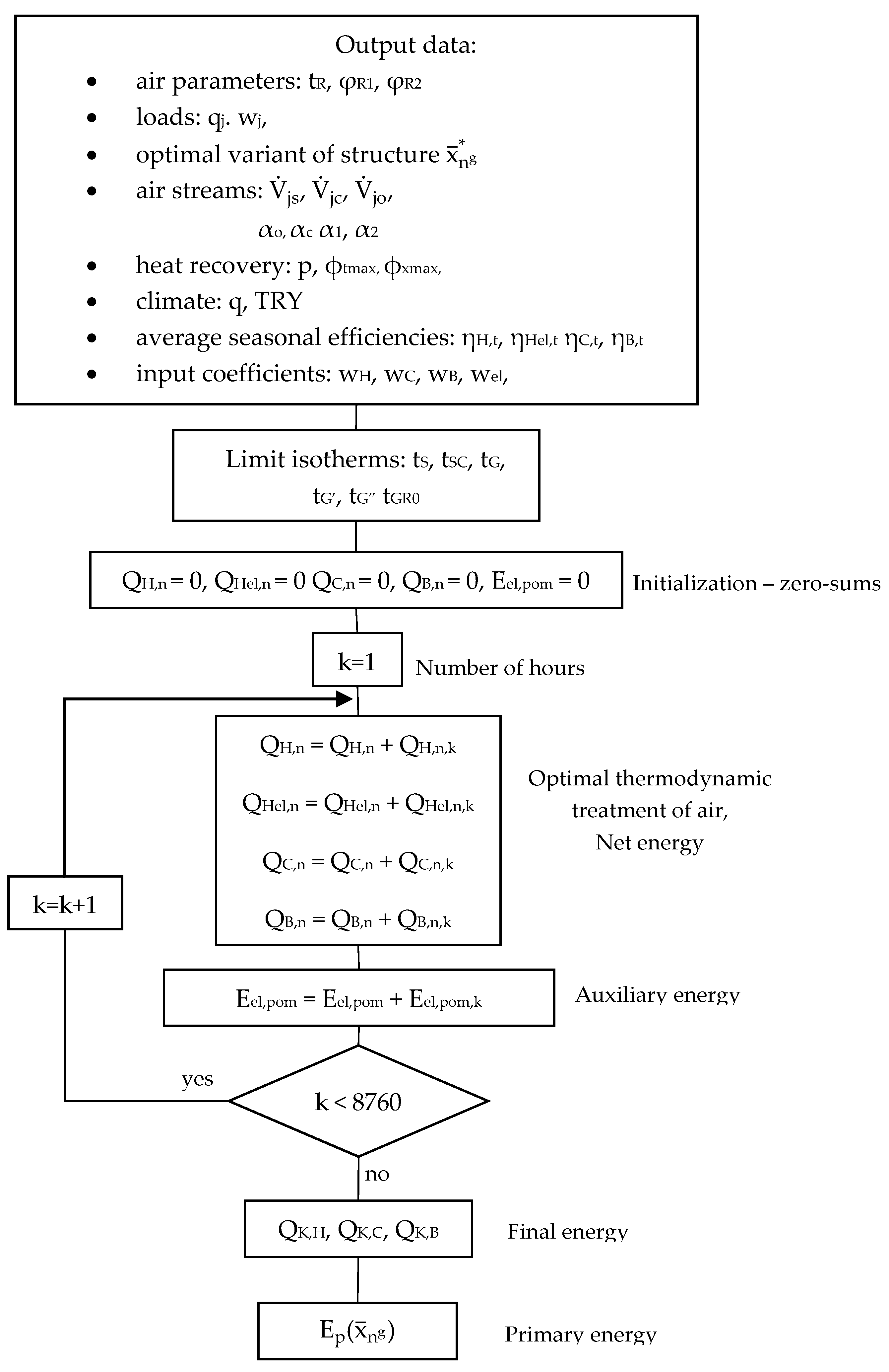
5.1. Objective Function, Simulation Models
- QH,n (QHel,n)—annual heat demand (net) of water heaters (electric heaters), kWh/ym2;
- QC,n—annual cold demand (net) of cooler, kWh/ym2;
- QB,n—annual heat demand (net) of steam humidifiers, kWh/ym2;
- QK,H (QK,Hel)—annual final energy demand of water heaters (electric heaters)—final heat kWh/ym2;
- QK,C—annual final energy demand of coolers—final cold, kWh/ym2;
- QK,B—annual final energy demand of steam humidifiers—final heat of humidifiers, kWh/ym2;
- Eel,pom—annual demand for final electrical energy for the drive of auxiliary devices, kWh/ym2;
- ηH,t—seasonal average total efficiency of a heating system with water air heaters, ηH,t = ηH,g ηH,s ηH,d ηH,e, with ηH,t = 0.81 (ηH,g = 0.90—generation, ηH,s = 1.0—accumulation, ηH,d = 0.94—distribution and ηH,e = 0.95—regulation and control);
- ηHel,t—seasonal average total efficiency of a heating system with electric heaters, with ηHel,t = 0.95;
- ηC,t—seasonal average total efficiency of a system with air coolers;ηC,t = ESEER ηC,s ηC,d ηC,e, with ηC,t = 3.0 (ESEER = 3.5—European Seasonal Energy Efficiency Ratio, ηC,s = 0.95—accumulation, ηC,d = 0.94—distribution and ηC,e = 0.97—regulation and control);
- ηB,t—seasonal average total efficiency of a heating system for supplying steam humidifiers, ηB,t = ηB,g ηB,d ηB,e (ηB,g—generation, ηB,d—distribution and ηH,e—regulation and control), with ηB,t = 0.95;
- wi—input coefficient of nonrenewable primary energy for generation and providing the final energy carrier (or energy) (wH—concerns heat, wC—concerns cold, wB—concerns steam, wel—concerns electrical energy) with wH = 1.1—gas/oil boiler, wC = 3.0—chiller with electrical drive and wB = 3.0—electric steam generator).
- —mass stream in i-operation;
- —change of the specific enthalpy in i-operation.
5.2. Objective Function, Simulation Models
- Air parameters in the room equal: tR = +22 °C, φR = (50 ± 5)%—φR1 = 45%, φR2 = 55%. Further parameters are included in Table 4.
- It is assumed that the gains in room humidity wj in relation to the air stream are negligible (xS = xR).
- The surface temperature of the cooler was assumed to be equal to tD = tDP − 1K.
- For HVAC systems and , and , and and and (with a crossflow or countercurrent exchanger), the outdoor air temperature at which frost occurs, equal to tGR0 = 0 °C, was used.
- The calculations were performed for three representative types of external climates according to Köppen [41]: continental with warm summer (q = 1), subarctic (q = 2) and subtropical (q = 3).
- Continuous operation of the HVAC system is assumed—τ = 24/7 with constant air streams.
- Final and primary energy demands for forcing through air (fans) are neglected, except for heat recovery exchangers, for which a realistic pressure loss of ∆pHR = 150 Pa and a total efficiency of forcing through ηW = 80% are used.
- ∆ER—final energy demand for forcing through by heat recovery exchangers.
- the objective function (29) is determined for each optimal structure of the HVAC system in which the location of the fans is specified; the energy demand of these fans does not therefore affect the selection of the optimal structure;
- determining the energy demand for fans would require assuming system pressure losses, which is not an objective parameter (such a possibility is provided for a case study);
- the purpose of the research at this stage is to determine the optimal type of heat recovery; to achieve this purpose, it is not necessary to determine the energy demand for the fans.
- 8.
- Annual demand for the final energy for the drive of auxiliary devices is neglected.
- 9.
- The following values of physical constants were used:air density ρ = 1.2 kg/m3, specific heat of air cp = 1.005 kg/kgK, specific heat of steam cpp = 1.86 kg/kgK, heat of vaporization of water with temperature 0 °C, ro = 2500.8 kJ/kg and atmospheric pressure pa = 105Pa.
- 10.
- Thermodynamic parameters of humid air were calculated based on Reference [42].
5.3. Algorithms of Energy-Optimal Control
- isotherm tS
- isotherm tSC
- isotherm tG
- isotherm tG′
- isotherm
- limit line (MR)C/(MR)CH2—
- limit line (MR)C/(MR)CH2—
- limit line C/CH2
- limit line (MR)C/(MR)CH2R—
- limit line (MR)C/(MR)CH2R—
- limit line CR/CH2R
5.4. Calculation Results, Interpretation
- 1.
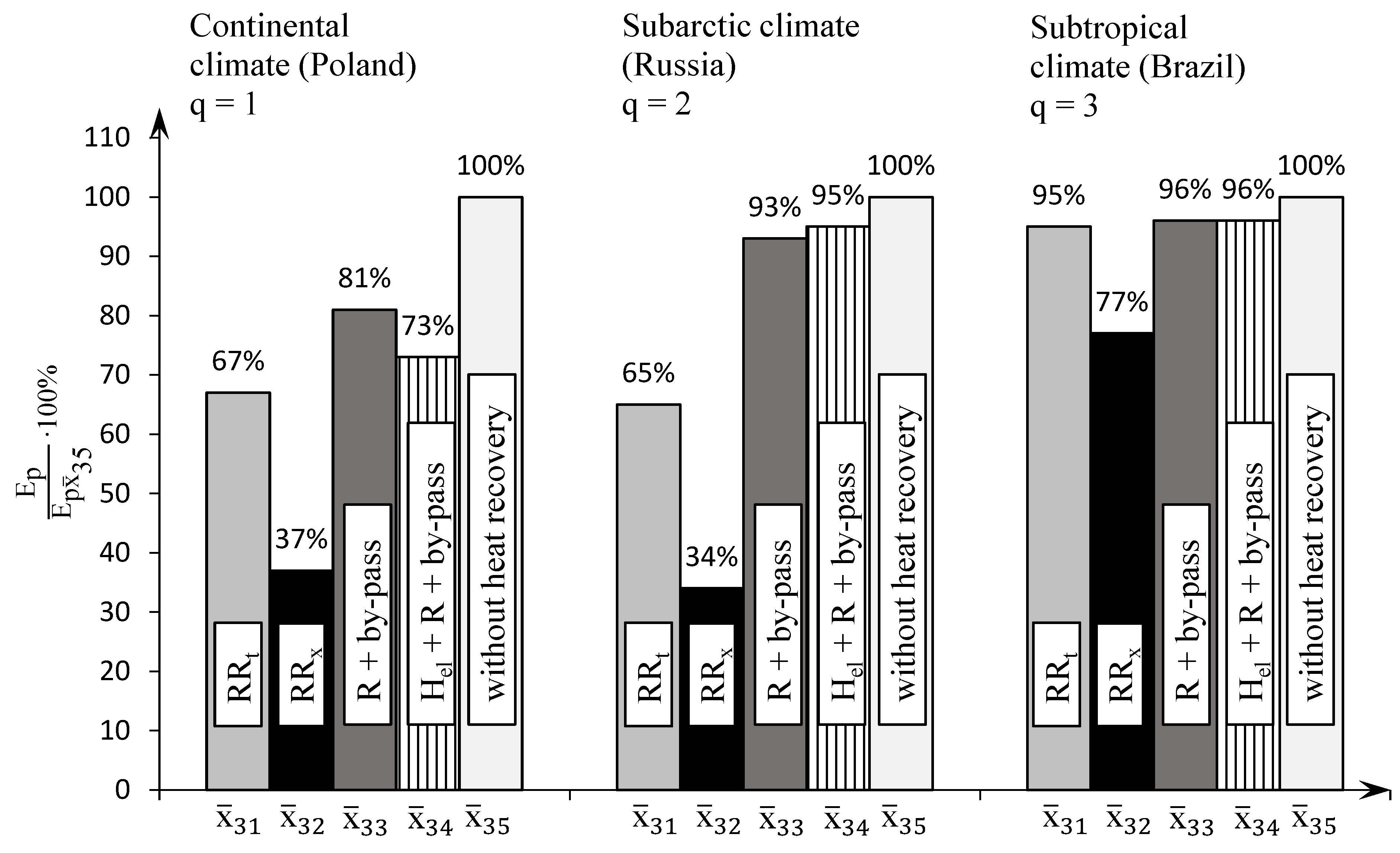
- For HVAC systems without air recirculation the optimal device for heat recovery is a rotary sorption regenerator (p = 2) and, then, an energy regenerator (p = 1) and a crossflow exchanger (p = 3 or p = 4). The obtained energy savings are here a function of climate—Figure 11 and Table 5.Using the rotary sorption regenerator in the analyzed HVAC system ISO8 makes it possible to decrease the annual primary energy demand by 63%, 64% and 24% in relation to the system without heat recovery, respectively, for continental (q = 1), subarctic (q = 2) and subtropical (q = 3) climates. For the rotary energy regenerator, the values are lower and equal 33%, 35% and 5%, respectively. For the crossflow exchanger, the savings are significantly lower and equal 19 ÷ 27% for the continental climate, 5 ÷ 7% for the subarctic climate and 4% for the subtropical climate. Therefore, in the subtropical climate, the only rational device for heat recovery is the rotary sorption regenerator, and the savings effect is mainly achieved by drying air.
- 2.
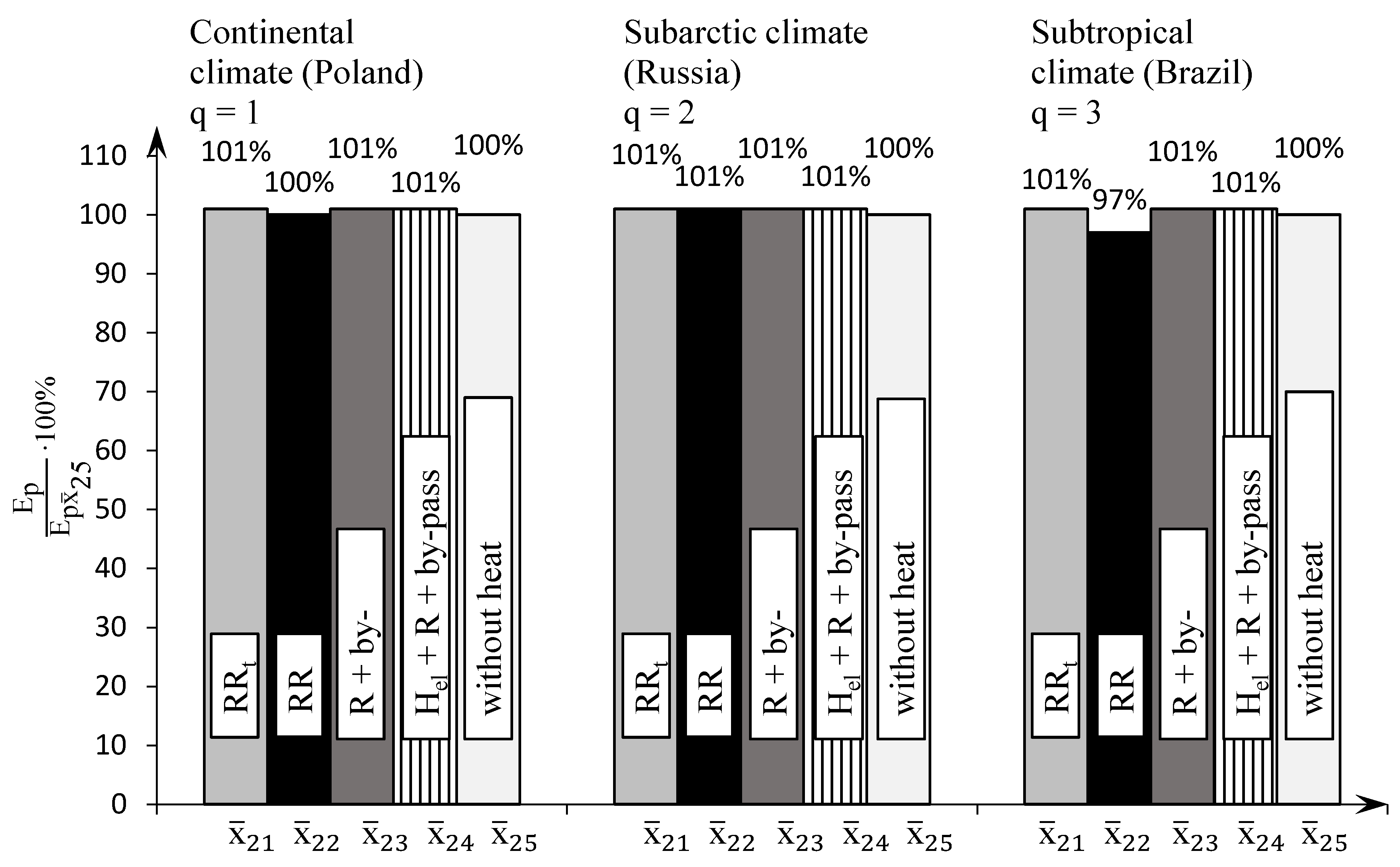
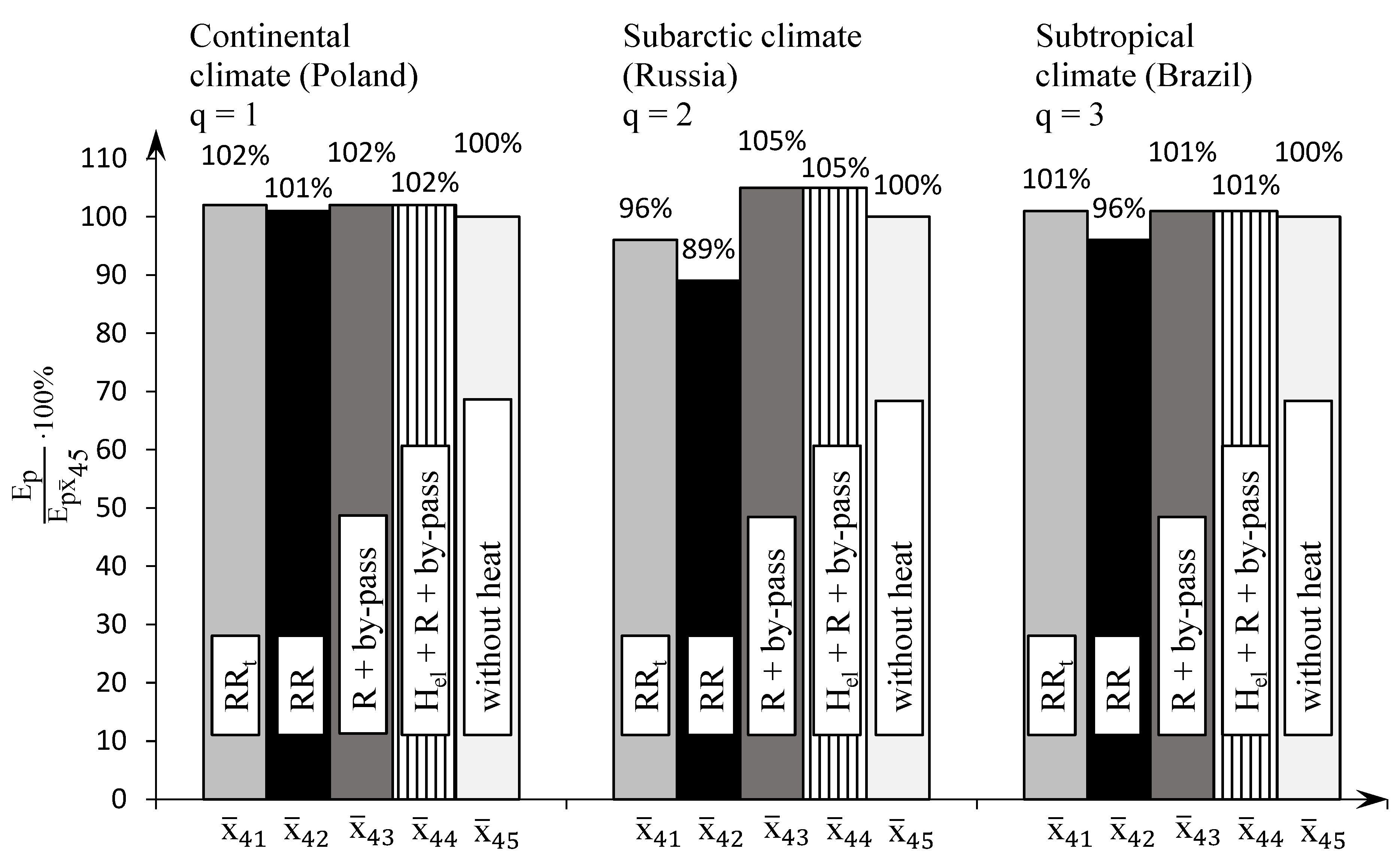
- For HVAC systems with external recirculation (optimal for cleanrooms with high unit cooling loads qj and relatively low requirements of cleanliness class Cs), using additional heat recovery has no energy justification for any of the considered devices and external climates (savings between 1 ÷ 3% for ISO8 )—Figure 12 and Table 5.
- 3.
- For systems with internal recirculation (optimal for cleanrooms with low cooling loads qj and relatively large percentages of outdoor air αo), using devices for heat recovery is definitely energetically justified, especially for the continental climate (q = 1) and the subarctic climate (q = 2)—Figure 13 and Table 5.The optimal device for heat recovery is, similar to the system without recirculation, a rotary sorption regenerator and, then, an energy regenerator and a crossflow exchanger. For the considered system ISO5 energy savings related to a system without heat recovery, primary energy and using the sorption regenerator equal 63%, 66% and 23%, respectively, for the continental, subarctic and subtropical climates—Figure 13.Lower savings are obtained by using an energy regenerator: 33%, 35% and 5% or a crossflow exchanger: 19 ÷ 27%, 5 ÷ 7% and 4%, respectively, for the continental, subarctic and subtropical climates.The percentages of the annual primary energy demand for thermodynamic air treatment for individual components (heaters, cooler and steam humidifier) of optimal variant ISO5 (with a sorption regenerator) and external climates are practically identical as for HVAC system (Figure 15).
- 4.
- For HVAC systems with external and internal recirculation (optimal for cleanrooms with high cooling loads qj and relatively low percentages of outdoor air αo), additionally using heat recovery is energetically justified only for the subarctic climate and concerns only the rotary sorption regenerator—Figure 14 and Table 5.Savings in the primary energy demand for the analyzed HVAC system ISO7 (with a sorption regenerator) and the subarctic climate equal 11% related to a system without heat recovery.
5.5. Validation of the Calculation Results
- it must be possible to implement the system structure in the program (in the case under consideration, four variants: , , and );
- it must be possible to implement various types of heat recovery along with control options: two-position control (maximum efficiency/0) and smooth control (variable energy-optimal efficiency);
- it must be possible to implement control algorithms (open code).
- no possibility to implement any HVAC system structure;
- no possibility to implement any control algorithms;
- frequently closed program code.
6. Conclusions
- it is energetically profitable to use heat recovery, especially for HVAC systems without recirculation () or with internal recirculation (), whereby the biggest energy savings are achieved for the continental climate (Poland) and the subarctic climate (Russia).
- in any case, the biggest savings in primary energy demand are the result of using, as heat recovery, a rotary sorption regenerator and, then, an energy regenerator and a crossflow (or countercurrent) exchanger.
- quantitatively, using a sorption regenerator in the energy-optimal structures of HVAC system ISO8 (without recirculation) and ISO5 (with internal recirculation) resulted in a decrease in the primary energy demand for thermodynamic treatment by 63%, 64 ÷ 66% and 23 ÷ 24%, respectively, for the continental, subarctic and subtropical climates. For an energy regenerator and a crossflow exchanger, these savings were significantly lower and equaled about 33%, 35% and 5%, respectively.
- for energy-optimal structures of HVAC systems with external recirculation or with external and internal recirculation using devices for heat recovery is generally energetically not justified and, in all cases, causes an increase in the energy demand (heat or cold recovery is lower than the energy inputs for forcing through by the heat recovery exchanger). The only debatable exception is the application of a sorption regenerator in the HVAC system for the subarctic climate—primary energy savings for thermodynamic air treatment of 11% in the ISO7 application .
Author Contributions
Funding
Institutional Review Board Statement
Informed Consent Statement
Data Availability Statement
Conflicts of Interest
Abbreviations
| AHU | Air-Handling Unit |
| MAU | Make-up Air-Handling Unit |
| RU (RDCU) | Return Unit (Return Dry Cooling Unit) |
| FFU (FDCU) | Filter Fan Unit (Fan Dry Cooling Unit) |
| DCC | Dry Cooling Coil |
| Cs | cleanliness class |
| E1, E2, E3 | efficiency of air filter of 1st, 2nd and 3rd stage |
| Eel,pom | annual demand for final electrical energy for the drive of auxiliary devices of HVAC system |
| EP | annual primary energy demand of HVAC system |
| k-limitation (T)—technological, (H)—hygienic, (A)—acoustic, (E)—energetic, (M) material, (AK)—architectural and constructional and (BN)—concerning safety and reliability [37] | |
| G | binary matrix of limitation conditions for matrix XJ |
| Gi | binary matrix of limitation conditions for matrix W |
| Gj | binary matrix of elimination of unnecessary decision variables for matrix (Gi × W) |
| kd | acceptable concentration of contaminants in room |
| air mass stream | |
| unit cooling load of room, W/m2 | |
| unit cooling load discharged using AHU, W/m2 | |
| unit cooling load of room discharged by the dry cooler in the internal recirculation circuit, W/m2 | |
| QH,n, QHel,n, QC,n, QB,n | net annual energy demand of heaters, electric heaters, coolers and steam humidifiers |
| QK,H, QK,C, QK,B | annual final energy demand of heaters (final heat), coolers (final cold) and steam humidifiers (final heat for humidifiers) |
| t | temperature, °C |
| tDP | dew point temperature |
| tG | outdoor air temperature (with percentage αo) for which the sensible heat gains are transferred without heat recovery (ϕt = 0), heating or cooling in AHU |
| tG′ | outdoor air temperature (with percentage αo) for which the sensible heat gains are transferred at maximal efficiency of heat recovery ϕt = ϕtmax but without heating air or cooling in AHU |
| tG″ | outdoor air temperature at which primary energy demand for the option of maximal heat and cold recovery (ϕt = ϕtmax) is equal to this demand for the heating-only option |
| tGR0 | outdoor air temperature limit below which the recuperator freezes |
| tS | air supply temperature |
| tSC | air supply temperature downstream AHU for which sensible heat gains are discharged from room as a result of mixing this air (with percentage αo) with internally recirculated air |
| tR | air temperature in room |
| Tu | turbulence degree |
| unit calculation ventilation air stream for cleanroom, m3/hm2 | |
| unit required air stream as function of room cleanliness class, m3/hm2 | |
| unit required air stream as function of cooling loads discharged using AHU, m3/hm2 | |
| unit required outdoor air stream, m3/hm2 | |
| w | average air speed in room |
| wi | input coefficient of nonrenewable primary energy for generation and supply of final energy carrier (or energy)—for balance boundary of building (wH—concerns heat for heaters, wC—concerns cold for coolers, wB—concerns heat for steam humidifiers and wel—concerns electrical energy) |
| Wi | binary matrix of all possible variants of combinations of decision variables values xj for normalizing constant parameter xi |
| W(Wg) | binary matrix of all possible variants (of acceptable variants) of combinations of decision variables values xj for normalizing all constant parameters xi of a HVAC system |
| xi | constant parameter of a HVAC system |
| xj | decision variable of a HVAC system |
| vector of a HVAC system | |
| binary vector defining the n-variant (ng-acceptable variant) of structure of a HVAC system used for normalizing all constant parameters | |
| vector of the optimal variant of HVAC system | |
| XJ(X) | binary matrix of all possible variants (of acceptable variants) of a HVAC system for normalizing constant parameters |
| αo (αos) | percentage of outdoor air compared to unit calculation air stream supplied to cleanroom (of unit required air stream as function of cleanliness class—) |
| αc | percentage of air being thermodynamically treated in AHU in air stream supplied to room— |
| α1, α2 | percentage of air under external recirculation, internal recirculation in air stream supplied to room— |
| εsdop | relative concentration of microorganisms |
| ηH,t, ηHel,t, ηC,t, ηB,t | seasonal average total efficiency of heating system for water heaters, heating system for electric heaters, cold system for coolers and heating system for steam humidifiers |
| φR | relative air humidity in room |
| ∆p | differential pressure (overpressure and underpressure in a room) |
| ∆h | change in specific enthalpy of the air |
| ϕt, ϕx | efficiency of sensible heat recovery, humidity |
| i | index of constant parameter of HVAC system |
| I | number of constant parameters of HVAC system |
| I* | number of normalized constant parameters of HVAC system |
| J | number of decision variables of HVAC system |
| k | index of k-combination of values of key constant parameters of HVAC system |
| K | number of combinations of values of key constant parameters of HVAC system |
| K | k-hour of reference year (TRY—Test Reference Year, k = 1 ÷ 8760) |
| kd | permissible concentration of pollutants |
| N | number of all possible variants of HVAC system for normalizing constant parameters |
Appendix A. Procedure for Determining the Matrix of Acceptable Variants of the HVAC System
- 1/—correlation with cleanliness class CS applies to special cases (DIN 1946-4:2018-09 [43]).
- XI*—binary matrix of normalized constant parameters xi of HVAC system,
- i = 1 … I*—number of normalized constant parameter,
- I*—number of normalized constant parameters of HVAC system,
- xi—constant parameter of HVAC system,
- —vector of normalized constant parameters of HVAC system.

- W—binary matrix of all possible variants of combinations of decision variables values xj for normalizing all constant parameters xi of HVAC system,
- xj—decision variable of HVAC system,
- j—index of decision variable of HVAC system,
- j*—index of decision variable of HVAC system from a universal set in Tables A2 and A3 [37],
- mi or r(i,mi)—index of mi- or r(i,mi)-variant of combinations of decision variables values xj for normalizing xi-constant parameter of HVAC system,
- Mi—number of all possible variants of combinations of decision variables values xj for normalizing xi-constant parameter of HVAC system,
- or —binary vector defining mi- or r(i, mi)-variant of combinations of decision variables values xj for normalizing xi-constant parameter of HVAC system (matrix element W).
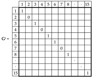
- Gi—binary matrix of limitation conditions for matrix W,
- —binary value in matrix of elimination of unnecessary decision variables Gi for r(i,mi)—variant of combinations of decision variables values xj for normalizing xi-constant parameter defined by vector in matrix W.

| r(i,mi) | Limitations g()k(xj) */ | Comments |
|---|---|---|
| 2 | gT6 | lack of a primary heater, with a large power differentiation for summer and winter, prevents the optimal selection of kV output coefficients of control valves for the secondary heater—and as a consequence causes unstable operation of control valves and extends the range of tolerance of the supply air temperature |
| gT19 | lack of a primary heater poses a risk of freezing of the water cooler | |
| 4 | gT11 gT28 | steam humidifier with lance in channel does not provide easy operational access to the humidification block for control and disinfection—difficulties in maintenance and decrease in safety |
| 7 | gT11 gT28 | steam humidifier with lance in channel does not provide easy operational access to the humidification block for control and disinfection—difficulties in maintenance and decrease in safety |

- Gj—binary matrix of elimination of unnecessary decision variables for matrix (Gi × W),

- Wg—binary matrix of acceptable variants of combinations of decision variables values xj for normalizing all constant parameters xi of HVAC system,
- or —binary vector defining mi- or r(i, mi)-variant r(i,)-acceptable variant) of combinations of decision variables values xj for normalizing xi-constant parameter of HVAC system (matrix element Wg),
- or r(i,)—index of - or r(i,)-variant of combinations of decision variables values xj for normalizing xi-constant parameter of HVAC system, after considering limitations.

- XJ—binary matrix of acceptable variants of HVAC system for normalizing constant parameters,
- —binary vector defining the n-variant of structure of HVAC system used for normalizing all constant parameters,
- or —binary value in the n-variant structures of HVAC system for - or r(i,)-variant of combinations of decision variables values for normalizing xi-constant parameter defined by vector or in matrix Wg, matrix element XJ,
- —number of all possible variants of combinations of decision variables values xj for normalizing xi-constant parameter of HVAC system, after considering limitations.
Limiting Conditions, Set of Acceptable Variants

- G—binary matrix of limitation conditions for matrix XJ,
- gnn—binary value in matrix with limitations G for the n-variant of structure of HVAC system defined by vector in matrix XJ,
| n | Comments |
|---|---|
| 1 | Variant thermodynamically identical to variant (n = 7), variant more favorable for the regulation of overpressure in the room |
| 2 | No consistency—∆p regulation—one air handling unit, α regulation—two air handling units |
| 3 | No consistency—∆p regulation—one air handling unit, α regulation—two air handling units |
| 4 | No consistency—∆p regulation—one air handling unit, α regulation—three air handling units |
| 6 | No consistency—∆p regulation—two air handling units in cascade, α regulation—one air handling unit |
| 9 | No consistency—∆p regulation—two air handling units in cascade, α regulation—three air handling units |
| 10 | Irrational variant—two air handling units (fans) in cascade in a system without recirculation |
| 11 | No consistency—∆p regulation—three air handling units, α regulation—one air handling unit |
| 12 | No consistency—∆p regulation—three air handling units, α regulation—two air handling units |
| 13 | No consistency—∆p regulation—three air handling units, α regulation—two air handling units |
| 15 | Irrational variant—three air handling units (fans) in cascade in a system without recirculation |

- X—binary matrix of acceptable variants of HVAC system for normalizing constant parameters,
- ( or )—binary value in the ng-acceptable variant structures of HVAC system for - or —variant of combinations of decision variables values for nor-malizing xi-constant parameter defined by vector or in matrix Wg, matrix element XJ,
- —binary vector defining the ng-acceptable variant of structure of HVAC system used for normalizing all constant parameters,
- n(ng)—index of the n-variant (of the ng-acceptable variant) of HVAC system.
References
- Kircher, K.; Shi, X.; Patil, S.; Zhang, K.M. Cleanroom energy efficiency strategies: Modeling and simulation. Energy Build. 2010, 42, 282–289. [Google Scholar] [CrossRef]
- Tschudi, W.; Xu, T. Cleanroom Energy Benchmarking Results. ASHREA Trans. 2003, 109, 733–739. [Google Scholar]
- Zhuang, C.; Shan, K.; Wang, S. Coordinated demand-controlled ventilation strategy for energy-efficient operation in multi-zone cleanroom air-conditioning systems. Build. Environ. 2021, 191, 107588. [Google Scholar] [CrossRef]
- Shan, K.; Wang, S. Energy efficient design and control of cleanroom environment control systems in subtropical regions—A comparative analysis and on-site validation. Appl. Energy 2017, 204, 582–595. [Google Scholar] [CrossRef]
- Tsao, J.-M.; Hu, S.-C.; Xu, T.; Chan David, Y.L. Capturing energy-saving opportunities in make-up air systems for cleanrooms of high-technology fabrication plant in subtropical climate. Energy Build. 2010, 42, 2005–2013. [Google Scholar] [CrossRef]
- Tsao, J.J.M.; Hu, S.-C.; Kao, W.-C.; Chien, L.-H. Clean Room Exhaust Energy Recovery Optimization Design. ASHRAE Trans. 2010, 116, 81–86. [Google Scholar]
- Hu, S.-C.; Chuah, Y.K. Power consumption of semiconductor fabs in Taiwan. Energy-Int. J. 2003, 28, 895–907. [Google Scholar] [CrossRef]
- Zhao, Y.; Li, N.; Tao, C.; Chen, Q.; Jiang, M. A comparative study on energy performance assessment for HVAC systems in high-tech fabs. J. Build. Eng. 2021, 39, 102188. [Google Scholar] [CrossRef]
- Hu, S.-C.; Lin, T.; Fu, B.-R.; Chang, C.-K.; Cheng, I.-Y. Analysis of energy efficiency improvement of high-tech fabrication plants. Int. J. Low-Carbon Technol. 2019, 14, 508–515. [Google Scholar] [CrossRef]
- Hu, S.-C.; Tsai, Y.-W.; Fu, B.-R.; Chang, C.-K. Assessment of the SEMI energy conversion factor and its application for semiconductor and LCD fabs. Appl. Therm. Eng. 2017, 121, 39–47. [Google Scholar] [CrossRef]
- Hu, S.-C.; Lin, T.; Huang, S.-H.; Fu, B.-R.; Hu, M.-H. Energy savings approaches for high-tech manufacturing factories. Case Stud. Therm. Eng. 2020, 17, 100569. [Google Scholar] [CrossRef]
- Lin, T.; Hu, S.-C.; Xu, T. Developing an innovative fan dry coil unit (FDCU) return system toimprove energy efficiency of environmental control for missioncritical cleanrooms. Energy Build. 2015, 90, 94–105. [Google Scholar] [CrossRef]
- Hu, S.-C.; Tsao, J.-M. A comparative study on energy consumption for HVAC systems of high-tech FABs. Appl. Therm. Eng. 2007, 27, 2758–2766. [Google Scholar] [CrossRef]
- Tsao, J.-M.; Hu, S.-C.; Chan, D.Y.L.; Hsu, R.T.C.; Lee, J.C.C. Saving Energy in the make-up unit (MAU) for semiconductor clean rooms in subtropical areas. Energy Build. 2007, 40, 1387–1393. [Google Scholar] [CrossRef]
- Kim, M.-H.; Kwon, O.-H.; Jin, J.-T.; Choi, A.-S.; Jeong, J.-W. Energy Saving Potentials of a 100% Outdoor Air System Integrated with Indirect and Direct Evaporative Coolers for Clean Rooms. J. Asian Archit. Build. Eng. 2012, 405, 1279–1285. [Google Scholar] [CrossRef] [Green Version]
- Yin, J.; Liu, X.; Guan, B.; Zhang, T. Performance and improvement of cleanroom environment control system related to cold-heat offset in clean semiconductor fabss. Energy Build. 2020, 224, 110294. [Google Scholar] [CrossRef]
- Yin, J.; Zhang, T.; Ma, Z.; Liu, X. Feasibility analysis of canceling reheating after condensation dehumidification in semiconductor cleanrooms. J. Build. Eng. 2021, 43, 102589. [Google Scholar] [CrossRef]
- Ma, Z.; Liu, X.; Zhang, T. Measurement and optimization on the energy consumption of fans in semiconductor cleanrooms. Build. Environ. 2021, 197, 107842. [Google Scholar] [CrossRef]
- Ma, Z.; Guan, B.; Liu, X.; Zhang, T. Performance analysis and improvement of air filtration and ventilation process in semiconductor clean air-conditioning system. Energy Build. 2020, 228, 110489. [Google Scholar] [CrossRef]
- Yin, J.; Liu, X.; Guan, B.; Ma, Z.; Zhang, T. Performance analysis and Energy saving potential of air conditioning system in semiconductor cleanrooms. J. Build. Eng. 2021, 37, 102158. [Google Scholar] [CrossRef]
- Chen, J.; Hu, S.-C.; Chien, L.-H.; Tsao, J.J.M.; Lin, T. Humidification of Large-Scale Cleanrooms by Adiabatic Humidification Method in Subtropical Areas: An Industrial Case Study. ASHRAE Trans. 2009, 115, 299–305. [Google Scholar]
- Xu, T.; Lan, C.-H.; Jeng, M.-S. Performance of large fan-filter units for cleanroom applications. Build. Environ. 2007, 42, 2299–2304. [Google Scholar] [CrossRef]
- Fan, M.; Cao, G.; Pedersen, C.; Lu, S.; Stenstad, L.-I.; Skogås, J.G. Suitability evaluation on laminar airflow and mixing airflow distribution strategies in operating rooms: A case study at St. Olavs Hospital. Build. Environ. 2021, 194, 107677. [Google Scholar] [CrossRef]
- Ozyogurtcu, G.; Mobedi, M.; Ozerdem, B. Economical assessment of different HVAC systems for an operating room: Case study for different Turkish climate regions. Energy Build. 2011, 43, 1536–1543. [Google Scholar] [CrossRef] [Green Version]
- Jia, L.; Liu, J.; Wei, S.; Xu, J. Study on the performance of two water-side free cooling methods in a semiconductor manufacturing factory. Energy Build. 2021, 243, 110977. [Google Scholar] [CrossRef]
- Zheng, G.; Li, X. Construction method for air cooling/heating process in HVAC system based on grade match between energy and load. Int. J. Refrig. 2021, 131, 10–19. [Google Scholar] [CrossRef]
- Wang, K.-J.; Dagne, T.B.; Lin, C.J.; Woldegiorgis, B.H.; Nguyen, H.-P. Intelligent control for energy conservation of air conditioning system in manufacturing systems. Energy Rep. 2021, 7, 2125–2137. [Google Scholar] [CrossRef]
- Zhuang, C.; Wang, S. Risk-based online robust optimal control of air-conditioning systems for buildings requiring strict humidity control considering measurement uncertainties. Appl. Energy 2020, 261, 114451. [Google Scholar] [CrossRef]
- Zhuang, C.; Wang, S.; Shan, K. Probabilistic optimal design of cleanroom air-conditioning systems facilitating optimal ventilation control under uncertainties. Appl. Energy 2019, 253, 113576. [Google Scholar] [CrossRef]
- Zhuang, C.; Wang, S.; Shan, K. Adaptive full-range decoupled ventilation strategy and air-conditioning systems for cleanrooms and buildings requiring strict humidity control and their performance evaluation. Energy 2019, 168, 883–896. [Google Scholar] [CrossRef]
- Zhuang, C.; Wang, S. An adaptive full-range decoupled ventilation strategy for buildings with spaces requiring strict humidity control and its applications in different climatic conditions. Sustain. Cities Soc. 2020, 52, 101838. [Google Scholar] [CrossRef]
- Chang, C.-K.; Lin, T.; Hu, S.-C.; Fu, B.-R.; Hsu, J.-S. Various Energy-Saving Approaches to a TFT-LCD Panel Fab. Sustainability 2016, 8, 907. [Google Scholar] [CrossRef] [Green Version]
- Loomans, M.G.L.C.; Molenaar, P.C.A.; Kort, H.S.M.; Joostenb, P.H.J. Energy demand reduction in pharmaceutical cleanrooms through optimization of ventilation. Energy Build. 2019, 202, 109346. [Google Scholar] [CrossRef]
- Loomans, M.G.L.C.; Ludlage, T.B.J.; van den Oever, H.; Molenaar, P.C.A.; Kort, H.S.M.; Joosten, P.H.J. Experimental investigation into cleanroom contamination build-up when applying reduced ventilation and pressure hierarchy conditions as part of demand controlled filtration. Build. Environ. 2020, 176, 106861. [Google Scholar] [CrossRef]
- Molenaar, P. Ventilation Efficiency Improvement in Pharmaceutical Cleanrooms for Energy Demand Reduction. Master’s Thesis, Eindhoven University of Technology, Eindhoven, The Netherlands, 2017. Available online: https://research.tue.nl/en/studentTheses/ventilation-efficiency-improvement-in-pharmaceutical-cleanrooms-f (accessed on 7 October 2021).
- Shao, X.; Liang, S.; Zhao, J.; Wang, H.; Fan, H.; Zhang, H.; Cao, G.; Li, X. Experimental investigation of particle dispersion in cleanrooms of electronic industry under different area ratios and speeds of fan filter units. J. Build. Eng. 2021, 43, 102590. [Google Scholar] [CrossRef]
- Porowski, M. The optimization method of HVAC system from a holistic perspective according to energy criterion. Energy Convers. Manag. 2019, 181, 621–644. [Google Scholar] [CrossRef]
- Porowski, M. Energy optimization of HVAC system from a holistic perspective: Operating theater application. Energy Convers. Manag. 2019, 182, 461–496. [Google Scholar] [CrossRef]
- ASHRAE. Chapter 18—Clean space. In ASHRAE Application Handbook; American Society of Heating, Refrigerating and Air-Conditioning Engineers Inc.: Atlanta, GA, USA, 2011. [Google Scholar]
- Xu, T. Characterization of minienvironments in a cleanroom: Assessing energy performance and its implications. Build. Environ. 2008, 43, 1545–1552. [Google Scholar] [CrossRef]
- Chen, D.; Chen, H. Using the Köppen classification to quantify climate variationand change: An example for 1901–2010. Environ. Dev. 2013, 6, 69–79. [Google Scholar] [CrossRef]
- Szczechowiak, E. Analityczne obliczanie parametrów powietrza wilgotnego. Chłodnictwo 1985, 20, 8. [Google Scholar]
- DIN 1946-4:2018-09 Ventilation and Air Conditioning—Part 4: Ventilation in Buildings and Rooms of Health Care. Available online: https://standards.globalspec.com/std/13389630/DIN1946-4 (accessed on 10 October 2021).


| Optimal Variant of the HVAC Structure | Relations: , and | Air Streams |
|---|---|---|
| αo = 1 i α1 = 0 i α2 = 0 , | ||
| , | ||
| , , | ||
| , |
| Variant of Constant Parameters | Cleanliness Class ISO(US.FSd.209e) | qj /6 W/m2 | αos /4 % | m3/hm2 | m3/hm2 | /7 m3/hm2 | Optimal Structure of HVAC System | |||||
|---|---|---|---|---|---|---|---|---|---|---|---|---|
m3/hm2 | αo /5 % | αc % | α1 % | α2 % | ||||||||
| 1.1.1 | ISO Class 5 1/ (M3.5—cl. 100) | 100 | 5 | 900 | 45 | 27.1 | 900 | 5 | 5 | - | 95 | |
| 1.1.2 | 10 | 900 | 90 | 27.1 | 900 | 10 | 10 | - | 90 | |||
| 1.1.3 | 30 | 900 | 270 | 27.1 | 900 | 30 | 30 | - | 70 | |||
| 1.1.4 | 50 | 900 | 450 | 27.1 | 900 | 50 | 50 | - | 50 | |||
| 1.1.5 | 100 | 900 | 900 | 27.1 | 900 | 100 | 100 | - | - | |||
| 1.2.1 | 300 | 5 | 900 | 45 | 81.4 | 900 | 5 | 9 | 4 | 91 | ||
| 1.2.2 | 10 | 900 | 90 | 81.4 | 900 | 10 | 10 | - | 90 | |||
| 1.2.3 | 30 | 900 | 270 | 81.4 | 900 | 30 | 30 | - | 70 | |||
| 1.2.4 | 50 | 900 | 450 | 81.4 | 900 | 50 | 50 | - | 50 | |||
| 1.2.5 | 100 | 900 | 900 | 81.4 | 900 | 100 | 100 | - | - | |||
| 1.3.1 | 500 | 5 | 900 | 45 | 135.7 | 900 | 5 | 15 | 10 | 85 | ||
| 1.3.2 | 10 | 900 | 90 | 135.7 | 900 | 10 | 15 | 5 | 85 | |||
| 1.3.3 | 30 | 900 | 270 | 135.7 | 900 | 30 | 30 | - | 70 | |||
| 1.3.4 | 50 | 900 | 450 | 135.7 | 900 | 50 | 50 | - | 50 | |||
| 1.3.5 | 100 | 900 | 900 | 135.7 | 900 | 100 | 100 | - | - | |||
| 2.1.1 | ISO Class 7 2/ (M5.5—cl.10 000) | 100 | 5 | 216 | 10.8 | 27.1 | 216 | 5 | 12.5 | 7.5 | 87.5 | |
| 2.1.2 | 10 | 216 | 21.6 | 27.1 | 216 | 10 | 12.5 | 2.5 | 87.5 | |||
| 2.1.3 | 30 | 216 | 64.8 | 27.1 | 216 | 30 | 30 | - | 70 | |||
| 2.1.4 | 50 | 216 | 108 | 27.1 | 216 | 50 | 50 | - | 50 | |||
| 2.1.5 | 100 | 216 | 216 | 27.1 | 216 | 100 | 100 | - | - | |||
| 2.2.1 | 300 | 5 | 216 | 10.8 | 81.4 | 216 | 5 | 37.7 | 32.7 | 62.3 | ||
| 2.2.2 | 10 | 216 | 21.6 | 81.4 | 216 | 10 | 37.7 | 27.7 | 62.3 | |||
| 2.2.3 | 30 | 216 | 64.8 | 81.4 | 216 | 30 | 37.7 | 7.7 | 62.3 | |||
| 2.2.4 | 50 | 216 | 108 | 81.4 | 216 | 50 | 50 | - | 50 | |||
| 2.2.5 | 100 | 216 | 216 | 81.4 | 216 | 100 | 100 | - | - | |||
| 2.3.1 | 500 | 5 | 216 | 10.8 | 135.7 | 216 | 5 | 62.8 | 57.8 | 37.2 | ||
| 2.3.2 | 10 | 216 | 21.6 | 135.7 | 216 | 10 | 62.8 | 52.8 | 37.2 | |||
| 2.3.3 | 30 | 216 | 64.8 | 135.7 | 216 | 30 | 62.8 | 32.8 | 37.2 | |||
| 2.3.4 | 50 | 216 | 108 | 135.7 | 216 | 50 | 62.8 | 12.8 | 37.2 | |||
| 2.3.5 | 100 | 216 | 216 | 135.7 | 216 | 100 | 100 | - | - | |||
| 3.1.1 | ISO Class 8 3/ (M6.5—cl.100 000) | 100 | 5 | 90 | 4.5 | 27.1 | 90 | 5 | 30 | 25 | 70 | |
| 3.1.2 | 10 | 90 | 9 | 27.1 | 90 | 10 | 30 | 20 | 70 | |||
| 3.1.3 | 30 | 90 | 27 | 27.1 | 90 | 30 | 30 | - | 70 | |||
| 3.1.4 | 50 | 90 | 45 | 27.1 | 90 | 50 | 50 | - | 50 | |||
| 3.1.5 | 100 | 90 | 90 | 27.1 | 90 | 100 | 100 | - | - | |||
| 3.2.1 | 300 | 5 | 90 | 4.5 | 81.4 | 90 | 5 | 90 | 85 | 10 | ||
| 3.2.2 | 10 | 90 | 9 | 81.4 | 90 | 10 | 90 | 80 | 10 | |||
| 3.2.3 | 30 | 90 | 27 | 81.4 | 90 | 30 | 90 | 60 | 10 | |||
| 3.2.4 | 50 | 90 | 45 | 81.4 | 90 | 50 | 90 | 40 | 10 | |||
| 3.2.5 | 100 | 90 | 90 | 81.4 | 90 | 100 | 100 | - | - | |||
| 3.3.1 | 500 | 5 | 90 | 4.5 | 135.7 | 135.7 | 3.3 | 100 | 96.7 | - | ||
| 3.3.2 | 10 | 90 | 9 | 135.7 | 135.7 | 6.6 | 100 | 93.4 | - | |||
| 3.3.3 | 30 | 90 | 27 | 135.7 | 135.7 | 19.9 | 100 | 80.1 | - | |||
| 3.3.4 | 50 | 90 | 45 | 135.7 | 135.7 | 33.2 | 100 | 66.8 | - | |||
| 3.3.5 | 100 | 90 | 90 | 135.7 | 135.7 | 100 | 100 | - | - | |||
| Cleanliness Class ISO 14644-1 (USFStd 209e) | W/m2 | m3/hm2 | m3/hm2 | αog % | W/m2 |
|---|---|---|---|---|---|
| ISO Class 5 (M 3.5—cl. 100) | 100 | 900 | 27.1 | 3 | 3300 */ |
| 300 | 81.4 | 9 | |||
| 500 | 135.7 | 15 | |||
| ISO Class 7 (M 5.5—cl. 10,000) | 100 | 216 | 27.1 | 12.5 | 796 */ |
| 300 | 81.4 | 37.7 | |||
| 500 | 135.7 | 62.8 | |||
| ISO Class 8 (M 6.5—cl. 100,000) | 100 | 90 | 27.1 | 30 | 332 |
| 300 | 81.4 | 90 | |||
| 500 | 135.7 | - **/ |
| Optimal Structure of HVAC System | Variant Designation | Variant of Constant Parameters 1/ | qj | αo | Heat Recovery | External Climate | |||
|---|---|---|---|---|---|---|---|---|---|
| W/m 2 | % | p 2/ | ϕt, % | ϕx, % | q 3/ | ||||
| ISO8 | 3.1.5 | 100 | 100 | 1 | 70 | 0 | 1,2,3 | ||
| 2 | 60 | ||||||||
| 3 | 0 | ||||||||
| 4 | 0 | ||||||||
| 5 | 0 | 0 | |||||||
| ISO8 | 3.3.3 | 500 | 19.9 | 1 | 70 | 0 | 1,2,3 | ||
| 2 | 60 | ||||||||
| 3 | 0 | ||||||||
| 4 | 0 | ||||||||
| 5 | 0 | 0 | |||||||
| ISO 5 | 1.2.3 | 300 | 30 | 1 | 70 | 0 | 1,2,3 | ||
| 2 | 60 | ||||||||
| 3 | 0 | ||||||||
| 4 | 0 | ||||||||
| 5 | 0 | 0 | |||||||
| ISO7 | 2.2.2 | 300 | 10 | 1 | 70 | 0 | 1,2,3 | ||
| 2 | 60 | ||||||||
| 3 | 0 | ||||||||
| 4 | 0 | ||||||||
| 5 | 0 | 0 | |||||||
| Optimal Structure of HVAC System | Heat Recovery (p) | Primary Energy Ep, kWh/m2y | |||
|---|---|---|---|---|---|
| Continental Climate (Poland) q = 1 | Subarctic Climate (Russia) q = 2 | Subtropical Climate (Brazil) q = 3 | |||
| ISO8 | ROt (p = 1) | 6354.0 | 9554.0 | 4877.0 | |
| ROx (p = 2) | 3464.0 | 5013.0 | 3915.0 | ||
| R + by-pass (p = 3) | 7643.0 | 13,693.0 | 4921.0 | ||
| Hel + R + by-pass (p = 4) | 6901.0 | 13,943.0 | 4921.0 | ||
| Without heat recovery (p = 5) | 9426.0 | 14,733.0 | 5118.0 | ||
| ISO8 | ROt (p = 1) | 4965.0 | 5078.0 | 5118.0 | |
| ROx (p = 2) | 4930.0 | 5055.0 | 4945.0 | ||
| R + by-pass (p = 3) | 4965.0 | 5078.0 | 5118.0 | ||
| Hel + R + by-pass (p = 4) | 4965.0 | 5078.0 | 5118.0 | ||
| Without heat recovery (p = 5) | 4898.0 | 5010.0 | 5091.0 | ||
| ISO5 | ROt (p = 1) | 19,053.0 | 28,656.0 | 14,634.0 | |
| ROx (p = 2) | 10,382.0 | 15,014.0 | 11,747.0 | ||
| R + by-pass (p = 3) | 22,883.0 | 41,033.0 | 14,686.0 | ||
| Hel + R + by-pass (p = 4) | 20,703.0 | 41,830.0 | 14,686.0 | ||
| Without heat recovery (p = 5) | 28,278.0 | 44,198.0 | 15,354.0 | ||
| ISO7 | ROt (p = 1) | 3071.0 | 3203.0 | 3159.0 | |
| ROx (p = 2) | 3040.0 | 2950.0 | 3000.0 | ||
| R + by-pass (p = 3) | 3070.0 | 3477.0 | 3159.0 | ||
| Hel + R + by-pass (p = 4) | 3070.0 | 3477.0 | 3159.0 | ||
| Without heat recovery (p = 5) | 3018.0 | 3322.0 | 3134.0 | ||
| Optimal Structure of HVAC System | Heat Recovery (p) | Primary Energy Ep, kWh/m2y | |||||||||
|---|---|---|---|---|---|---|---|---|---|---|---|
| External Climate (q) | |||||||||||
| Continental Climate (Poland) q = 1 | Subarctic Climate (Russia) q = 2 | Subtropical Climate (Brazil) q = 3 | |||||||||
| Simulation | HAP Carrier | Difference */ % | Simulation | HAP Carrier | Difference */ % | Simulation | HAP Carrier | Difference */ % | |||
| IOS8 | ROt (p = 1) | 6354.0 | 6402.0 | +0.75 | 9554.0 | 10,408.0 | +8.2 | 4877.0 | 4466.0 | −8.4 | |
| ROx (p = 2) | 3464.0 | 3212.0 | −7.3 | 5013.0 | 4623.0 | −7.8 | 3915.0 | 3656.0 | −6.6 | ||
| R + by-pass (p = 3) | 7643.0 | 7231.0 | −5.3 | 13,693.0 | 14,530.0 | +5.7 | 4921.0 | 4466.0 | −9.2 | ||
| Without heat recovery (p = 5) | 9426.0 | 9408.0 | −0.2 | 14,733.0 | 15,961.0 | +7.7 | 5118.0 | 4819.0 | −6.0 | ||
| IOS8 | ROt (p = 1) | 4965.0 | 5231.0 | +5.0 | 5078.0 | 4849.0 | −4.5 | 5118.0 | 5106.0 | −0.2 | |
| ROx (p = 2) | 4930.0 | 5178.0 | +4.8 | 5055.0 | 4592.0 | −9.2 | 4945.0 | 4533.0 | −8.3 | ||
| R + by-pass (p = 3) | 4965.0 | 5244.0 | +5.3 | 5078.0 | 4849.0 | −4.5 | 5118.0 | 5106.0 | −0.2 | ||
| Without heat recovery (p = 5) | 4898.0 | 5170.0 | +5.3 | 5010.0 | 4886.0 | −2.5 | 5091.0 | 5084.0 | −0.1 | ||
Publisher’s Note: MDPI stays neutral with regard to jurisdictional claims in published maps and institutional affiliations. |
© 2022 by the authors. Licensee MDPI, Basel, Switzerland. This article is an open access article distributed under the terms and conditions of the Creative Commons Attribution (CC BY) license (https://creativecommons.org/licenses/by/4.0/).
Share and Cite
Porowski, M.; Jakubiak, M. Energy-Optimal Structures of HVAC System for Cleanrooms as a Function of Key Constant Parameters and External Climate. Energies 2022, 15, 313. https://doi.org/10.3390/en15010313
Porowski M, Jakubiak M. Energy-Optimal Structures of HVAC System for Cleanrooms as a Function of Key Constant Parameters and External Climate. Energies. 2022; 15(1):313. https://doi.org/10.3390/en15010313
Chicago/Turabian StylePorowski, Mieczysław, and Monika Jakubiak. 2022. "Energy-Optimal Structures of HVAC System for Cleanrooms as a Function of Key Constant Parameters and External Climate" Energies 15, no. 1: 313. https://doi.org/10.3390/en15010313
APA StylePorowski, M., & Jakubiak, M. (2022). Energy-Optimal Structures of HVAC System for Cleanrooms as a Function of Key Constant Parameters and External Climate. Energies, 15(1), 313. https://doi.org/10.3390/en15010313