Abstract
Vehicle speed prediction plays a critical role in energy management strategy (EMS). Based on the adaptive particle swarm optimization–least squares support vector machine (APSO-LSSVM) algorithm with BP neural network (BPNN), a novel closed-loop vehicle speed prediction system is proposed. The database of a vehicle internet platform was adopted to construct a speed prediction model based on the APSO-LSSVM algorithm. Furthermore, a BPNN is established according to the local high-precision nonlinear fitting relationship between the predicted value and error so as to correct the prediction value. Then, the results are returned to the APSO-LSSVM model for calculating the minimum fitness function, thus obtaining a closed-loop prediction system. Finally, equivalent fuel consumption minimization strategy (ECMS) based EMS was performed. According to the simulation results, the RMSE performance is 0.831 km/h within 5 s, which is over 20% higher than other performances. Additionally, the training time is 15 min within 5 s, which is advantageous over BPNN. Furthermore, fuel consumption increases by 6.95% compared with the dynamic-programming algorithm and decreased by 5.6%~10.9% compared with the low accuracy of speed prediction. Overall, the proposed method is crucial for optimizing EMS as it is not only effective in improving prediction accuracy but also capable of reducing training time.
1. Introduction
Currently, electric passenger cars have been increasingly popularized, which aim to reduce oil consumption while simultaneously addressing air pollution [1]. However, for electric heavy trucks, the main downside of short endurance mileage results in declining sales. Despite the capability of advanced battery storage system to ensure the sufficient mileage of heavy trucks, this type of battery remains immature and has not been verified in real-world conditions [2]. As a promising direction of transport electrification, fuel cell hybrid vehicle (FCHV) has been drawing widespread attention for research studies across the automotive industry due to advantages such as zero emission, low noise and high efficiency [3]. Therefore, fuel cell and electric battery technologies are considered as practical solutions for zero emission.
As far as heavy trucks are concerned, the diversity of region, time and environment results in complex driving conditions, which presents new challenges to the implementation of an adaptable and optimal energy management strategy (EMS) [4]. Particularly for FCHV, given the immaturity of existing technology and the high cost of fuel, high-efficiency EMS can not only minimize fuel consumption but also extends the service life of components [5].
Currently, rule-based EMS and optimization-based EMS have been widely adopted [6]. For the former, its development relies heavily on engineering experience, which makes it difficult to develop a better rule for adapting to different driving habits and conditions. For the latter, an attempt was made to solve the problem with energy management from the perspective of optimal control based on the pre-knowledge of exact driving conditions [7]. Similarly, it is challenging to adapt to complex driving conditions due to the diversity of region, time and environment. For instance, in literature [8], global optimization control can be applied to optimize the most reasonable EMS when the overall driving conditions are determined. However, when the quality of various devices, such as sensors, CAN buses and communication networks, is affected by the working environment or hardware conditions, the actual driving conditions are changeable, which affects the optimized results. Therefore, both of the methods as mentioned above are unable to produce the expected effect in energy conservation [9].
With the development of intelligent transportation and vehicle network technology, the approach to collecting driving information has been increasingly diversified [10], which presents an opportunity to execute an adaptable and optimal energy management strategy in practice. In this context, an optimal and real-time energy management prediction control model has emerged and has been commonly applied [11,12], which makes vehicle speed prediction an essential module.
According to the means of data collection as adopted in the future vehicle prediction conditions, it can be divided into real-time learning prediction and offline learning prediction [13]. The former is based on external real-time information, which is sourced from the intelligent transportation system or front vehicle data in queue environment. In [14], a model was proposed to achieve predictive control based on positioning information of the navigation system. In [15], speed information based on the Internet of Vehicles was used to predict short-term working conditions. Jonsson proposed predicting future working conditions by using a prediction method based on driving information of the front vehicle [16]. In [17], a NNTM-SP algorithm was put forward to predict the vehicle speed profile with traffic information. In [18], a new vehicle speed prediction controller was proposed using the tire-road friction coefficient and the GPS signal, which is essential for the energy management of hybrid vehicles. Offline learning prediction is made on the basis of historical information, which is a method where its own historical operating condition is taken as the basis of prediction [19]. In [20], a Markov chain method was applied to predict future driving conditions by using the stochastic process of driving conditions. In [21,22], the transfer probability matrix was adopted to construct a Markov prediction model on the basis of vehicle speed. Additionally, a high-order Markov speed predictor was designed with the assistance of linear programming algorithm [23]. Nevertheless, the Markov method suffers problems such as low prediction accuracy and the inability to simulate dynamic driving behavior [24]. Despite the capability of the high-order Markov method to improve the accuracy of prediction, the model is highly complex. Due to the complex nonlinear spatial problem facing vehicle speed prediction, some scholars proposed improving the accuracy of prediction using machine learning methods, such as NN and SVM [25]. In [26], a deep learning method of neural networks was proposed for predicting vehicle speed. However, the method was excessively reliant on driving data, which affects the accuracy of prediction. Murphey et al. constructed a self-learning neural network model for the prediction of working conditions, and this model was trained using the data collected from road information and traffic flow parameter [27]. Moreover, in [28], the long-term and short-term neural network was introduced to predict the trend of variation in traffic flow using the traffic flow data. Developed by Ma et al., the LSTM-NN prediction method demonstrated its advantage in prediction accuracy and the consistency of performance for long-term time series prediction [29]. However, the prediction ability of the neural network was clearly restricted by fitting, which results in significant prediction error. Moreover, the required training time was longer. Showing an excellent learning ability and a high speed of convergence, support vector machine (SVM) is obviously advantageous in solving the problems with finite samples and nonlinear regression estimations. In [30], a novel transit flow prediction model was proposed on the basis of LSSVM, with the result showing little difference between the prediction value and the actual value. In [31,32], the working conditions were identified by LSSVM as optimized by grid search and cross validation (CV). Unfortunately, the parameters used to optimize LSSVM are time consuming.
To sum up, there are two perspectives from which this problem can be addressed. One is the accuracy of prediction. The other is training time. It seems that all of the prediction models proposed so far have the advantages and disadvantages of their own. It is worth noting that a potential solution to these issues is to explore the effective methods of prediction that can incorporate their merits while compensating for the weakness of each other. Focusing on the characteristics of LS-SVM and BP neural networks, this paper proposes a novel closed-loop system intended for vehicle speed prediction based on the adaptive particle swarm optimization–least squares support vector machine (APSO-LSSVM) and BP neural network (BPNN). In order to achieve this goal, firstly, a vehicle speed prediction model was first established using LS-SVM based on the historical driving conditions as collected by a vehicle-mounted TBOX. Then, an adaptive particle swarm algorithm was applied as the rolling optimization strategy to identify the optimal parameter for the LS-SVM algorithm. Afterwards, a BP neural network was constructed to establish a local high-precision nonlinear fitting relationship between the predicted value and deviation, thus achieving a correction of prediction value. Finally, the results were returned to the APSO model for calculating the minimum fitness function so as to obtain the best γ and σ. According to the simulation results, the closed-loop system used for vehicle speed prediction system can achieve higher prediction accuracy with reasonable training time required. The main contributions of this paper are reflected in the following two points. On the one hand, a novel closed-loop system intended for vehicle speed prediction was proposed according to APSO-LSSVM and BPNN, which laid the foundation for designing and optimizing energy management strategies. On the other hand, the conflict arising between LSSVM and BPNN toolboxes, which were used repeatedly in MATLAB, was resolved.
The remainder of this article is organized as follows. In Section 2, an introduction will be made for the source of driving cycle data experiments. In Section 3, an introduction is provided for the novel closed-loop prediction model on the basis of APSO LSSVM and BP-NN. Meanwhile, ECMS-based EMS with vehicle speed prediction is presented. The simulation is carried out in Section 4, which is followed by comparative analysis and discussion. Finally, conclusions are presented in Section 5.
2. Driving Cycle Data Experiments
2.1. Vehicle Structure and Paramerter
As the research objective in this paper, the configuration of the FCHV heavy-duty truck is illustrated in Figure 1. The parallel FCHV consists of a fuel cell engine system, DCDC, hydrogen system, power distribution (PDU), battery, motor controller unit (MCU), motor, vehicle controller unit (VCU) and other components. DCDC converter plays a significant role in addressing the voltage difference between the output voltage of the fuel cell engine system and the battery system, which ensures not only that the vehicle drive motor always works in the best working range but also that the fuel cell output voltage is unaffected by other external conditions. The working principle is detailed as follows. Hydrogen and oxygen in the air undergo an electrochemical reaction in the fuel cell engine system. Then, the generated electric energy is boosted by DCDC, which is combined with the power battery and transmitted to the driving motor, thus driving the vehicle. At this time, the excess electric energy is transferred to the power battery for storage. The main parameters of the vehicle are listed in the Table 1.
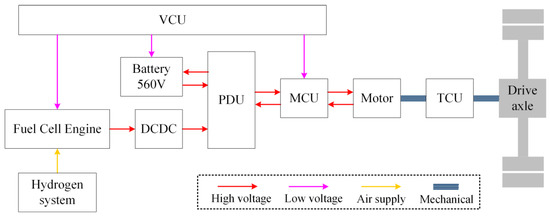
Figure 1.
Schematic of the FCHV configuration.

Table 1.
Vehicle parameters.
2.2. Data Acquisition Based on Internet of Vehicles
The hydrogen fuel cell hybrid (FCHV) heavy-duty truck studied in this paper is intended specifically for an enterprise based in Shanghai to carry out cargo transportation. A representative operating route that involves urban roads, expressway and highway was selected as the test object for acquiring the original driving conditions. Given peak traffic and external environments that result in diverse and complex driving conditions, it is crucial to ensure the accuracy of driving data. Therefore, a telematics box (TBOX) fitted with a global positioning system (GPS) was used to collect the current instantaneous speed driving conditions from the wheel speed sensor by CAN bus in the FCHV vehicle, and the collected data are uploaded to the background databases through a wireless network, which can reflect line traffic conditions and the characteristics of vehicle driving. In addition, the better the quality of the data, the more complete the data information becomes, and the more objective the characteristics it indicates.
Based on the above-mentioned methods, it is necessary to monitor and manage the vehicles for at least one month in order to capture sufficient characteristics of vehicle speed along the route. In this paper, the database of five vehicles was downloaded from the Internet of Vehicles, and the vehicle daily driving route in Shanghai is shown in Figure 2. The driving route of the vehicle stretches between two points, such as A and B; A and C; A and E; and A and F. A denotes the starting point, which is in Baoshan district, while B, C, D, E and F refer to the different destination points of the five vehicles, respectively. More details about the five-point vehicles can be found in Table 2, including urban road distance, expressway and highway distance, traffic lights, vehicle license plate and vehicle position.
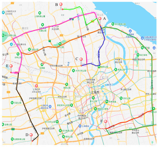
Figure 2.
Daily driving route in Shanghai.
Table 2.
Detailed information for the five vehicles.
The driving data collected for six days are shown in Figure 3, which includes working time and speed information of the vehicle in a week. It can be observed from the figure that the average daily working time is 10 h. The mean speed does not exceed 40 km/h on urban roads. Moreover, the mean speed does not exceed 65 km/h on the expressway and highway. Obtained by using the vehicle speed integration process, driving mileage can reach up to 350 km. By using an analysis of the six-day driving data collected from different vehicles, it can be observed that a fixed speed characteristic is reflected in different road sections. In the next section, collected data are processed by using data analysis as preparation for the subsequent prediction of speed.
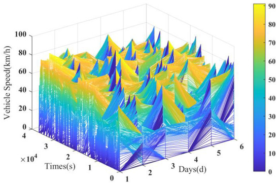
Figure 3.
Driving speeds under the fixed route of six days.
2.3. Data Processing
High-quality data are considered a prerequisite for the discovery and acquisition of knowledge. In this paper, the quality of various devices, such as sensors, CAN buses and communication networks, is susceptible to the impact of different factors including working environment, hardware conditions and operating costs. Therefore, the acquired driving data suffer quality problems to varying degrees. By conducting analysis on driving data, it was found that data noise is the main quality problem. In the following part, a discussion is conducted about processing data quality.
Wavelet filtering can be performed to obtain the low-frequency and high-frequency components at a preset scale. This method is effective in decomposing noise data while retaining all of original information. Therefore, wavelet filtering was performed in this paper to achieve data denoising.
The discrete wavelet transform (DWT) function can be expressed as Equation (1):
where the step size is a fixed value that is greater than 1; and is a fixed value that is greater than 0.
The DWT coefficients can be expressed as Equation (2).
According to the famous Mallat algorithm, scale coefficients () and wavelet coefficients () can be obtained using the scale coefficient of and the following Equation (3):
where is the low-pass wavelet filter coefficient, while is the high-pass filter coefficient. can be confirmed by [33].
The reconstruction of DWT is shown in Equation (4).
According to the above-mentioned step, vehicle speed and acceleration compared with the reference data curve are determined by wavelet decomposition, respectively. Figure 4 shows a certain section of the entire working condition. The red curves are the original vehicle speed and acceleration, respectively. The blue curves (WF) are the results based on wavelet filtering. It is evident that most of the vehicle speed spikes have been blunted, with the acceleration reflected in real time. Finally, the signal was reconstructed, and complete driving conditions were obtained.
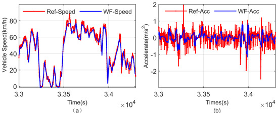
Figure 4.
Partial perspective view of wavelet denoising. (a) Vehicle speed; (b) Accelerate.
3. Vehicle Speed Prediction Method
In the previous section, the acquisition and processing of driving cycle data based on the Internet of Vehicles have been completed. Therefore, a description is made in this section of the characteristics and environment under which APSO-LSSVM and BP-NN are designed for vehicle speed prediction. Moreover, an introduction is made in detail of the novel closed-loop system built for vehicle speed prediction model on the basis of APSO LSSVM and BP-NN. Furthermore, ECMS is introduced to construct the energy management strategy.
3.1. APSO LSSVM Prediction Method
3.1.1. LSSVM Prediction Method
LSSVM refers to a machine learning process commonly used as an effective prediction tool in engineering settings. The training samples of the prediction model are set as , where represents the input vector of the n-dimensional samples, while refers to output vector. In the high dimensional feature space of Hilbert, the LSSVM model can be expressed as Equation (5):
where represents weight vector, indicates bias vector and denotes mapping performed from low dimensional space to high dimensional space.
According to the principle of structural risk minimization, the optimal regression estimation of the LSSVM is conducted by calculating the minimization functional with certain constraints. The minimization functional can be expressed as Equation (6):
where is the error vector, and is a positive penalty term.
In order to solve the optimization problem, the Lagrange multiplier () is introduced to construct the function, as shown in Equation (7).
The best and best can be obtained under Karush–Kuhn–Tucker (KKT) conditions. Moreover, the final linear equations can be obtained as Equation (8):
where , , , and is the unit matrix. represents the square matrix, which is constructed by the kernel function.
The prediction model of LSSVM can be expressed as Equation (9):
where represents the radial basis function, which was treated as the kernel function, and refers to the width of Gaussian kernel.
3.1.2. Parameter Optimization of APSO-LSSVM
The values of penalty parameter and kernel width parameter in LSSVM are related to its generalization ability. However, the traditional search process can be performed only on grid points, which is time consuming as a result. In order to resolve this nonlinear optimization problem, the adaptive particle swarm optimization (APSO) algorithm was applied in this paper, with a large-scale global search and quasi-Newton local search method adopted to find the best parameters.
In the APSO algorithm, where represents the position vector of the particle, and where represents the best position of the particle.
The speed and position should be updated using Equation (10):
where and represent learning factors, usually , indicates the inertia weight, represents the best individual position and refers to the best global position.
The inertia weight () adaptive strategy can be expressed as Equation (11):
where represents the max inertia weight, indicates the min inertia weight, denotes the maximum number of iterations run and stands for the current number of iterations.
In order to keep population diversity effective, the following method expressed as Equation (12) was used to determine whether the particle mutated:
where represents the Euclidean distance of particle and , as shown in Equation (13):
where indicates similarity, which is supposed to follow the judgment criteria: if , then ; if , then ; .
Finally, some parameters of the APSO-LSSVM model used in this paper are listed in Table 3.
Table 3.
APSO-LSSVM model parameters.
3.2. BP Neural Network Prediction Method
As a feed forward neural network based on the correction of errors, a BP neural network can be applied as a suitable model for dealing with relevant issues by adjusting the number of hidden layers, the number of the neurons and the learning algorithm. In general, it includes three or more layers, namely, the input layer, the hidden layer and the output layer. A three-layer BP neural network model was adopted in this paper to ensure high performance in predicting nonlinear relationships.
The output layer neuron can be expressed as Equation (14):
where represents the number of input layer nodes; indicates the number of hidden layer nodes; denotes the activation function, ; refers to the state vector which is passed from the input layer; and denote the thresholds of the output layer and hidden layer, respectively; stands for the synapse weight between the hidden layer and the output layer; and indicates the synapse weight between the input layer and the hidden layer.
Obtained by comparing the expected output () with the actual output , the error e can be expressed as . The synapse weight represented by and is re-updated by the error layer-by-layer until the error falls within an acceptable range.
Figure 5 shows the structure of the vehicle prediction model based on the BP neural network. The left diagram shows the learning procedure, while the right diagram shows the prediction procedure, and indicates the final results of the prediction. The parameters of the BP model used in this paper are listed in Table 4.
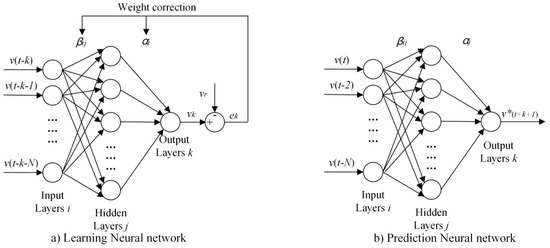
Figure 5.
Structure of BP neural network. (a) Learning neural network; (b) prediction neural network.
Table 4.
BP NN model parameters.
3.3. A Closed-Loop Vehicle Speed Prediction System
The prediction models, as mentioned above, can rely on the predicted road driving conditions; it remains necessary to improve the accuracy of prediction models. By analyzing the characteristics of each prediction model, it can be found that a potential solution is to explore effective prediction methods, which can incorporate their intrinsic advantages while compensating for the drawbacks of each other. Therefore, a novel closed-loop vehicle speed prediction system based on APSO-LSSVM and BP neural network was proposed, as shown in Figure 6. The details are shown below.
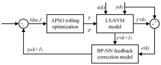
Figure 6.
Predictive control model based on APSO LSSVM and BPNN.
Based on the proposed method, the nonlinear prediction model is established, as shown in Equation (15):
where represents the input vector of the vehicle speed predictive model; indicates the output vector; and and denote the number of the input and output vector, respectively.
For the nonlinear system, the system output is when the input control variable is . With the history vehicle speed substituted into the LSSVM prediction model, the estimated output of the system can be obtained as . In order to optimize system input , the output value of the system is estimated. Due to noise interference or model mismatch and other reasons, however, it is common for deviation to occur between the predicted model output and the actual output . The prediction deviation at time can be written as . BP-NN was adopted to establish a nonlinear fitting relationship between the predicted value and the deviation , thus achieving feedback correction of the predicted value. The correction function is expressed as Equation (14). Then, APSO was used to calculate the minimum value of the fitness function, as shown in Equation (16). Then, the best and best were obtained to support the LS-SVM predictive model. Processing was repeated until the minimum fitness was achieved. Considering a conflict between the toolbox of BP and LSSVM in the MATLAB, the command of ‘addpath’ and ‘rmpath’ should be a looping execution for avoiding wrong pauses in operation.
The predictive control algorithm based on APSO LSSVM and BPNN involves the following steps:
- Parameters initialization. Set PSO algorithm, LSSVM model and BPNN model parameters;
- Construction of the vehicle speed prediction LSSVM model. Train the training samples set and make predictions on the test samples set;
- Correction by BPNN algorithm. The error of k time and the prediction value of time are obtained by the LSSVM model. BP-NN is applied to establish the local high-precision nonlinear fitting relationship between the predicted value and error, thus obtaining the correction value of time;
- Calculation of the fitness functions and updating the best parameters by APSO algorithm. The parameters and of LSSVM are set as the position vectors of the particles in the PSO. The fitness value of each particle is calculated using Equation (16), while the individual optimal and global optimal of the particle are compared and updated;
- Update the velocity and position. Use Equation (10) to recalculate the velocity and position of the particles;
- Randomly mutate position. Calculate the similarity between each particle and the optimal particle , with the particle position randomly mutated according to Equation (12);
- Compared and update. Perform comparison with the fitness of each particle and update the optimal value of the particle and ;
- APSO algorithm termination criteria. If the number of iterations is smaller than the set maximum value or the error parameter is lower than the set error value, the best output parameters and should be acted on LSSVM model. Then, the BP-NN output is treated as the prediction result. Otherwise, revert to step 4 until the end of the control.
3.4. Energy Management Strategy (EMS) with Speed Prediction
In order to meet the demands of driver power while simultaneously achieving the optimum vehicle fuel economy, EMS must be designed to adjust the distribution of power between the fuel cell engine and the battery electrical energy at any time under the real-world road conditions. Combined with closed-loop vehicle speed prediction, an equivalent fuel consumption minimization strategy (ECMS) was introduced in this section to achieve the optimum fuel economy.
Based on Pontryagin’s maximum principle (PMP) [34], EMCS is a local real-time optimization method that can be applied to convert electric energy consumption into equivalent hydrogen fuel consumption by using an equivalent factor when the global driving condition is unknown. On the basis of meeting the constraints of the fuel cell hybrid power system, the instantaneous equivalent fuel consumption of the fuel cell hybrid power system can be minimized. The core idea of PMP is to make the optimal control variable satisfy the Hamiltonian function that is minimized. The Hamiltonian function can be defined as Equation (17):
where represents hydrogen consumption, which involves equivalent hydrogen consumption by the fuel cell and battery, refers to the state of charge of the battery, which is the state variable, stands for the power of battery, which is control variable, denotes the co-state, indicates the hydrogen consumption rate by fuel cell, represents the equivalent hydrogen consumption rate by battery, represents a function of the state variable () and the control variable (), which can be expressed as Equation (18):
where indicates the open circuit voltage of battery, denotes internal resistance, represents the battery efficiency and refers to the capacity of the battery.
Both and have an energy conversion relationship with power, which can be expressed as Equation (19):
where indicates the driver’s demand power, refers to the DCDC efficiency, denotes the fuel cell engine efficiency, LHV is the low heat value of the hydrogen and LHV = 120 MJ/kg.
According to the principle of PMP, the optimal control sequence with constraint conditions can be formulated as Equation (20):
where refers to the terminal state of the battery, denotes the initiate state of battery, indicates the power of the fuel cell engine power, denotes the rate of the fuel cell power change and min and max stand for the minimum and maximum values of the corresponding parameters, respectively.
The partial derivatives of and can be expressed as Equation (21).
In order to resolve the nonlinear optimization problem as mentioned above, the dynamic programming (DP) algorithm based on the Behrman optimization principle is employed. The process of DP is detailed in Figure 7. Herein, s indicates the state variable (), u denotes the control variable () and refers to the cost function of the k-th step time, which can be calculated by Equation (17).
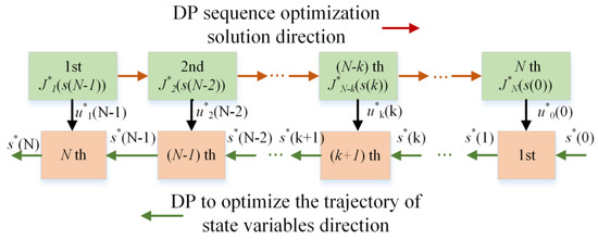
Figure 7.
Solution process of dynamic programming algorithm.
4. Results and Discussion
4.1. Performance of Prediction Evaluation
In order to validate the novel closed-loop vehicle speed prediction system based on APSO-LSSVM and BP neural networks, simulation was performed with the assistance of MATLAB. The training sample sets are one of the six-day driving conditions, while the information collected on the other days is treated as the test sample sets for verifying the prediction effect.
Figure 8 shows speed prediction results and prediction error of four methods, including BP-NN, LSSVM, APSO-LSSVM and the closed-loop prediction system based on APSO-LSSVM and BP-NN. In order to visualize the above prediction performance more intuitively, these images were partially enlarged, as shown in Figure 9. Table 5 shows the performances of these four methods in different time domains.
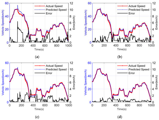
Figure 8.
The speed prediction results and prediction error of four methods. (a) BPNN speed prediction; (b) LSSVM speed prediction; (c) APSO LSSVM speed prediction; (d) APSO LSSVM and BP NN speed prediction.
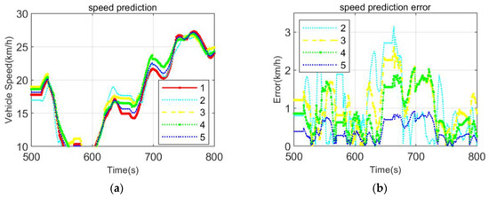
Figure 9.
Partial magnification of speed prediction results. (a) Vehicle speed prediction; (b) Vehicle speed prediction error.
Table 5.
The assessment at different time domain.
The red line in Figure 8 indicates the reference vehicle’s speed, while the blue and black lines represent prediction results and absolute value of the prediction error, respectively. Upon a comparison between (a) and (b), it can be found that BP-NN has more significant errors than LSSVM. Obviously, the LSSVM prediction model had higher accuracy when the vehicle was in the deceleration phase (259 s–288 s), which indicates that LSSVM exhibited greater sensitivity to the change in speed. Distinctly, the BP neural network prediction model produced a better effect when the vehicle was in the fluctuation phase (800 s–864 s), indicating that BP neural network performed better in fitting given the local variation. Thus, it can be judged that both of the prediction models have the advantages of their own. As for the overall effect of the error simulation, however, LSSVM algorithm had a less significant error, suggesting better generalization ability than the BP neural network. Figure 8c shows APSO-LSSVM optimization results. Upon a comparison between Figure 8b,c, it can be found that the effect of error simulation is basically the same. Both of them can follow the reference speed strictly. Figure 8d presents a diagram showing closed-loop vehicle speed prediction effects. Compared with other diagrams, it can be clearly observed that the predicted curve almost overlaps with the reference curve, with the error falling below 1 km/h. By comparing high-speed area with the low-speed area, it can be discovered that the accuracy of high-speed predictions is higher than the low-speed predictions in all methods and all vehicle speed horizons, which is attributed to the fact that low-speed conditions are mostly caused by external environmental restrictions, which result in highly complex calculations and lower accuracy of the prediction. Therefore, it can be concluded that the accuracy of the prediction by BP-NN is the worst among all methods. The novel closed-loop vehicle speed prediction system has better generalization ability than others, while there is no significant prediction accuracy difference between LSSVM and APSO-LSSVM.
Figure 9 shows a partial enlargement of the images. The number ranging from one to five represents the reference speed, the BP neural network, the LSSVM, the APSO LSSVM and the APSO LSSVM and BP NN, respectively. As shown in the figure, BP-NN has a strong capability of training prediction as the speed changes. The detailed view of LSSVM and APSO-LSSVM has more regular prediction results compared with BP-NN, which is due to the fact that they belong in supervised learning. The novel closed-loop vehicle speed prediction system can master acceleration variations of the vehicle more precisely and is more sensitive to changes in speed, which results in smoother prediction curves than compared to other methods. It can be concluded that not only does the novel closed-loop system perform better in generalization ability, it also reduces the range of fluctuation for the error than compared to others prediction models. That is to say that the proposed prediction model can improve prediction accuracy by incorporating the advantages of the single model and compensating for the weakness of each other.
The difference in time domain of prediction has a significant impact on the accuracy of prediction. Therefore, in order to further evaluate the accuracy of prediction and the training time for these four methods, the evaluation indexes of the parameters in different time domains of prediction were compared, as shown in Table 5. According to the horizontal comparison performed in the first set of the predictions, the MAE in the BPNN, LSSVM and the APSO LSSVM prediction model within 5 s is 1.011 km/h, 0.9243 km/h and 0.923 km/h, respectively. Comparatively, it is 0.714 km/h in the closed-loop vehicle speed prediction system, which indicates the better generalization ability of the proposed method than others. Relative to RMSE performance, the closed-loop prediction model achieves an improvement by 30%, 23% and 23%, respectively. By comparison with training times, it can be discovered that BPNN requires a longer training time due to the slow pace of convergence. Moreover APSO-LSSVM can produce a better performance, and eliminates the risk of lengthiness and blindness encountered by the conventional cross-validation method. Statistically, the proposed method takes 15 min, which is 30% shorter than BPNN. As revealed by a longitudinal comparison in the closed-loop system, with the increase in time domain, the error increases progressively. Meanwhile, the cost of the training time increases as well, which is because the increasing model output quantity results in complex processes of model training.
4.2. Simulation for EMS
The simulation of EMS validation was conducted on the Matlab/Simulink platform. In this paper, a DP-based EMS and the ECMS-based EMS with the vehicle speed prediction methods of APSO-LSSVM, BP-NN and a closed-loop prediction system were constructed. Figure 10 show driving speed and driving distance. Figure 11 shows the state of charge SOC. Figure 12 shows the changes in equivalent hydrogen fuel consumption. Table 6 lists the results of EMS simulation.
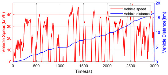
Figure 10.
Driving speed and driving distance.
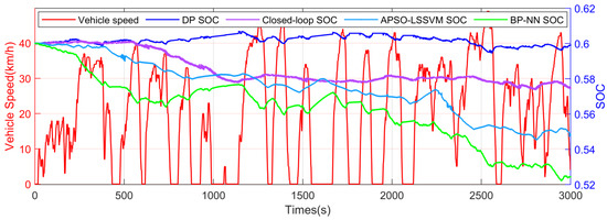
Figure 11.
State of charge of SOC with vehicle speed.
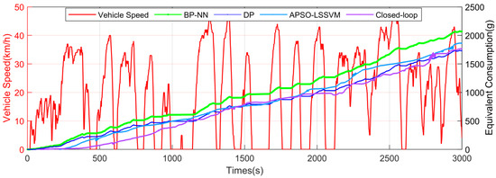
Figure 12.
Changes of equivalent hydrogen fuel consumption.
Table 6.
EMS simulation results.
Figure 10 shows speed and distance, from which it can be observed that the driving distance is 16.49 km. Figure 11 shows the state of charge. Obviously, the SOC trajectory of DP-EMS is based on a global optimization algorithm for the global planning of power usage, in addition to the optimal SOC trajectory, is obtained, with a relatively slight variation. In contrast, other methods alternately utilize the charge depleting mode and the charge sustaining mode, which is attributed to the fewer global information about the driving cycle. Closed-loop-based EMS and APSO-LSSVM-based EMS show a gentle curve when the fuel cell engine runs with maximum efficiency. Since BPNN-based EMS has a relatively large variation, there is a nearly linear decrease. As can be observed in Figure 12 and Table 6, with a global optimal algorithm used, DP achieves the best hydrogen economy with an equivalent fuel consumption of only 10.5 kg/100 km. The closed-loop vehicle speed prediction system based ECMS, which has the best accuracy of the prediction, achieved an equivalent fuel consumption of 11.23 kg/100 km, which is 6.95% higher than the DP algorithm and decreased by 5.6~10.9% compared with the low accuracy of speed prediction. Since BP-NN performs worst in speed prediction, the equivalent fuel consumption is 12.6 kg/100 km, and the APSO-LSSVM is better than BP-NN, with an equivalent fuel consumption of 11.9 kg/100 km.
5. Conclusions
In this paper, a novel closed-loop vehicle speed prediction system based on the APSO-LSSVM and BP NN was proposed to improve the EMS of the fuel cell hybrid heavy truck. Firstly, with the fixed route of a special truck operated by a company in Shanghai as the research object, vehicle driving cycle information was collected from the Internet of Vehicles platform. Then, a wavelet filtering algorithm was applied for the purpose of data denoising. Afterwards, the advantages of APSO-LSSVM and BP neural network were incorporated to design the closed-loop vehicle speed prediction model. Furthermore, ECMS was conducted to verify fuel economy. Finally, simulation was conducted using different methods, which resulted in results suggesting that RMSE performance of the closed-loop vehicle speed prediction system is 0.831 km/h within 5 s, which is more than 20% higher than others. Moreover, the training time is 15 min within 5 s, which is superior to BPNN. In addition, with the time domain increasing, the error increases as well. While the accuracy of prediction decreases. Furthermore, the equivalent hydrogen fuel consumption increases by only 6.95% when compared with the dynamic-programming algorithm and decreased by 5.6~10.9% when compared with the low accuracy of speed prediction. In summary, the closed-loop system intended for vehicle speed prediction model can take full advantage of the BP neural network and APSO LSSVM while compensating for the defects of each other, which is essential for vehicle speed prediction and energy optimization of the FCHV.
In the future, more deep-learning models intended for vehicle speed prediction will be combined to further improve the accuracy of prediction and reduce training time.
Author Contributions
Conceptualization, X.G., X.Y., Z.C. and Z.M.; methodology, X.G.; software, X.G. and Z.M.; validation, X.G. and Z.M.; formal analysis, X.G. and Z.M.; investigation, X.G. and Z.M.; resources, X.G. and Z.M.; data curation, X.G. and Z.M.; writing—original draft preparation, X.G. and Z.M.; writing—review and editing, X.G. and Z.M.; visualization, X.G.; supervision, X.Y. and Z.C. All authors have read and agreed to the published version of the manuscript.
Funding
This research has been supported by funding from the Shanxi Provincial Department of Science and Technology Major Special Project “Hydrogen Consumption Analysis and Energy Management of Hydrogen Fuel Cell Heavy Trucks” grant number 20181102009.
Institutional Review Board Statement
Not applicable.
Informed Consent Statement
Not applicable.
Data Availability Statement
Data and codes used for this research could be shared with the research community upon request to the corresponding author.
Acknowledgments
The authors want to thank the Shanghai Horizon Co., Ltd., for collecting and sharing the dataset used in this study. The authors want to thank the JMC Heavy Duty Vehicle Co., Ltd., for providing the fuel cell heavy truck. The authors want to thank the Shanxi Setan Defense Technology Co., Ltd., for supporting of software.
Conflicts of Interest
The authors declare no conflict of interest.
References
- Liu, Y.; Liu, J.; Zhang, Y.; Wu, Y.; Chen, Z.; Ye, M. Rule learning based energy management strategy of fuel cell hybrid vehicles considering multi-objective optimization. Energy 2020, 207, 118212. [Google Scholar] [CrossRef]
- Nassif, G.G.; de Almeida, S.C. Impact of powertrain hybridization on the performance and costs of a fuel cell electric vehicle. Int. J. Hydrogen Energy 2020, 45, 21722–21737. [Google Scholar] [CrossRef]
- Fathabadi, H. Combining a proton exchange membrane fuel cell (PEMFC) stack with a Li-ion battery to supply the power needs of a hybrid electric vehicle. Renew. Energy 2019, 130, 714–724. [Google Scholar] [CrossRef]
- Lee, D.Y.; Elgowainy, A.; Kotz, A.; Vijayagopal, R.; Marcinkoski, J. Life-cycle implications of hydrogen fuel cell electric vehicle technology for medium- and heavy-duty trucks. J. Power Sources 2018, 393, 217–229. [Google Scholar] [CrossRef]
- Teng, T.; Zhang, X.; Dong, H.; Xue, Q. A comprehensive review of energy management optimization strategies for fuel cell passenger vehicle. Int. J. Hydrogen Energy 2020, 45, 20293–20303. [Google Scholar] [CrossRef]
- Olatomiwa, L.; Mekhilef, S.; Ismail, M.S.; Moghavvemi, M. Energy management strategies in hybrid renewable energy systems: A review. Renew. Sustain. Energy Rev. 2016, 62, 821–835. [Google Scholar] [CrossRef]
- Peng, J.; He, H.; Xiong, R. Rule based energy management strategy for a series–parallel plug-in hybrid electric bus optimized by dynamic programming. Appl. Energy 2017, 185, 1633–1643. [Google Scholar] [CrossRef]
- Yuan, J.; Yang, L.; Chen, Q. Intelligent energy management strategy based on hierarchical approximate global optimization for plug-in fuel cell hybrid electric vehicles. Int. J. Hydrogen Energy 2018, 43, 8063–8078. [Google Scholar] [CrossRef]
- Zhang, L.; Liu, W.; Qi, B. Combined Prediction for Vehicle Speed with Fixed Route. Chin. J. Mech. Eng. 2020, 33, 33–60. [Google Scholar] [CrossRef]
- Wang, Y.; Zeng, X.; Song, D.; Yang, N. Optimal rule design methodology for energy management strategy of a power-split hybrid electric bus. Energy 2019, 185, 1086–1099. [Google Scholar] [CrossRef]
- Yan, M.; Li, M.; He, H.; Peng, J. Deep Learning for Vehicle Speed Prediction. Energy Procedia 2018, 152, 618–623. [Google Scholar] [CrossRef]
- Yao, G.; Du, C.; Ge, Q.; Jiang, H.; Wang, Y.; Ait-Ahmed, M.; Moreau, L. Traffic-Condition-Prediction-Based HMA-FIS Energy-Management Strategy for Fuel-Cell Electric Vehicles. Energies 2019, 12, 4426. [Google Scholar] [CrossRef] [Green Version]
- Wang, Y. Research on Intelligent Energy Management Strategy for Hybrid Electric Bus Based on Vehicular Network Information. Ph.D. Thesis, Jilin University, Changchun, China, 2020. [Google Scholar]
- Ichikawa, S.; Yokoi, Y.; Doki, S.; Okuma, S.; Naitou, T.; Shiimado, T.; Miki, N. Novel energy management system for hybrid electric vehicles utilizing car navigation over a commuting route. IEEE Intell. Veh. Symp. 2004, 2004, 161–166. [Google Scholar]
- Alshayeb, S.; Stevanovic, A.; Park, B.B. Field-Based Prediction Models for Stop Penalty in Traffic Signal Timing Optimization. Energies 2021, 14, 7431. [Google Scholar] [CrossRef]
- Jonsson, J.; Jansson, Z. Fuel Optimized Predictive Following in Low Speed Conditions. IFAC Proc. 2004, 37, 119–124. [Google Scholar] [CrossRef] [Green Version]
- Park, J.; Li, D.; Murphey, Y.L.; Kristinsson, J.; McGee, R.; Kuang, M.; Phillips, T. Real time vehicle speed prediction using a Neural Network Traffic Model. In Proceedings of the IEEE The 2011 International Joint Conference on Neural Networks, San Jose, CA, USA, 31 July–5 August 2011; pp. 2991–2996. [Google Scholar]
- Li, L.; Coskun, S.; Zhang, F.; Langari, R.; Xi, J. Energy Management of Hybrid Electric Vehicle Using Vehicle Lateral Dynamic in Velocity Prediction. IEEE Trans. Veh. Technol. 2019, 68, 3279–3293. [Google Scholar] [CrossRef]
- Li, Y.; Peng, J.; He, H.; Xie, S. The Study on Multi-scale Prediction of Future Driving Cycle Based on Markov Chain. Energy Procedia 2017, 105, 3219–3224. [Google Scholar] [CrossRef]
- Xie, S.; Hu, X.; Liu, T.; Qi, S.; Lang, K.; Li, H. Predictive vehicle-following power management for plug-in hybrid electric vehicles. Energy 2019, 166, 701–714. [Google Scholar] [CrossRef]
- Kolmanovsky, I.; Siverguina, I.; Lygoe, B. Optimization of powertrain operating policy for feasibility assessment and calibration: Stochastic dynamic programming approach. In Proceedings of the IEEE American Control Conference, Anchorage, AK, USA, 8–10 May 2002; pp. 1425–1430. [Google Scholar]
- Lin, C.C.; Peng, H.; Grizzle, J.W. A stochastic control strategy for hybrid electric vehicles. In Proceedings of the IEEE American Control Conference, Boston, MA, USA, 30 June–2 July 2004; pp. 4710–4715. [Google Scholar]
- Kim, M.J. Modeling, Control, and Design Optimization of a Fuel Cell Hybrid Vehicle. Ph.D. Thesis, University of Michigan, Ann Arbor, MI, USA, 2007. [Google Scholar]
- Zhou, Y.; Ravey, A.; Péra, M.-C. Multi-objective energy management for fuel cell electric vehicles using online-learning enhanced Markov speed predictor. Energy Convers. Manag. 2020, 213, 112821. [Google Scholar] [CrossRef]
- Lin, C.C. Modeling and Control Strategy Development for Hybrid Vehicles. Ph.D. Thesis, University of Michigan, Ann Arbor, MI, USA, 2004. [Google Scholar]
- Xie, H. A Research on Driving Condition Prediction for HEVs Based on Markov Chain. Ph.D. Thesis, Chongqing University, Chongqing, China, 2013. [Google Scholar]
- Yavasoglu, H.A.; Tetik, Y.E.; Ozcan, H.G. Neural network-based energy management of multi-source (battery/UC/FC) powered electric vehicle. Energy Res. 2020, 44, 12416–12429. [Google Scholar] [CrossRef]
- Chen, X.; Chen, H.; Yang, Y.; Wu, H.; Zhang, W.; Zhao, J.; Xiong, Y. Traffic flow prediction by an ensemble framework with data denoising and deep learning model. Phys. A Stat. Mech. Its Appl. 2021, 565, 125574. [Google Scholar] [CrossRef]
- Murphey, Y.L.; Chen, Z.; Kiliaris, L.; Park, J.; Kuang, M.; Masrur, A.; Phillips, A. Neural Learning of Driving Environment Prediction for Vehicle Power Management. In Proceedings of the 2008 IEEE International Joint Conference on Neural Networks, Hong Kong, China, 1–8 June 2008; pp. 3755–3761. [Google Scholar]
- Ma, X.; Tao, Z.; Wang, Y.; Yu, H.; Wang, Y. Long short-term memory neural network for traffic speed prediction using remote microwave sensor data. Transp. Res. Part C Emerg. Technol. 2015, 54, 187–197. [Google Scholar] [CrossRef]
- Chen, Q.; Li, W.; Zhao, J. The use of LS-SVM for short-term passenger flow prediction. Transport 2011, 26, 5–10. [Google Scholar] [CrossRef]
- Zheng, Y.; He, F.; Shen, X.; Jiang, X. Energy Control Strategy of Fuel Cell Hybrid Electric Vehicle Based on Working Conditions Identification by Least Square Support Vector Machine. Energies 2020, 13, 426. [Google Scholar] [CrossRef] [Green Version]
- Zandi, A.S.; Moradi, M.H. Quantitative evaluation of a wavelet-based method in ventricular late potential detection. Pattern Recognit. 2006, 39, 1369–1379. [Google Scholar] [CrossRef]
- Xing, J.; Chu, L.; Guo, C.; Pu, S.; Hou, Z. Dual-Input and Multi-Channel Convolutional Neural Network Model for Vehicle Speed Prediction. Sensors 2021, 21, 7767. [Google Scholar] [CrossRef]
Publisher’s Note: MDPI stays neutral with regard to jurisdictional claims in published maps and institutional affiliations. |
© 2021 by the authors. Licensee MDPI, Basel, Switzerland. This article is an open access article distributed under the terms and conditions of the Creative Commons Attribution (CC BY) license (https://creativecommons.org/licenses/by/4.0/).