Abstract
With the development of autonomous driving technology, the requirements for machine perception have increased significantly. In particular, camera-based lane detection plays an essential role in autonomous vehicle trajectory planning. However, lane detection is subject to high complexity, and it is sensitive to illumination variation, appearance, and age of lane marking. In addition, the sheer infinite number of test cases for highly automated vehicles requires an increasing portion of test and validation to be performed in simulation and X-in-the-loop testing. To model the complexity of camera-based lane detection, physical models are often used, which consider the optical properties of the imager as well as image processing itself. This complexity results in high efforts for the simulation in terms of modelling as well as computational costs. This paper presents a Phenomenological Lane Detection Model (PLDM) to simulate camera performance. The innovation of the approach is the modelling technique using Multi-Layer Perceptron (MLP), which is a class of Neural Network (NN). In order to prepare input data for our neural network model, massive driving tests have been performed on the M86 highway road in Hungary. The model’s inputs include vehicle dynamics signals (such as speed and acceleration, etc.). In addition, the difference between the reference output from the digital-twin map of the highway and camera lane detection results is considered as the target of the NN. The network consists of four hidden layers, and scaled conjugate gradient backpropagation is used for training the network. The results demonstrate that PLDM can sufficiently replicate camera detection performance in the simulation. The modelling approach improves the realism of camera sensor simulation as well as computational effort for X-in-the-loop applications and thereby supports safety validation of camera-based functionality in automated driving, which decreases the energy consumption of vehicles.
1. Introduction
The traffic safety problem is severe with an increasing number of vehicles on the road. According to [1], approximately 11 percent of road accidents result from lane departures caused by inattentive, distracted, or drowsy drivers. According to statistics from [2], in 2015 nearly 13,000 people died in single-vehicle run-off-road, head-on, and sideswipe crashes where a passenger vehicle left the lane without warning. Lane Keeping Assist (LKA) and lane departure warnings are designed to reduce potential risk and improve driving safety. They support more effective driving tasks that maintain safe lateral vehicle control. The study that investigated the safety potential of Lane Keeping Assist systems shows that the possibility to avoid fatal accidents is between 16.4% and 29.2%, depending on the capability of the system [3]. For passenger vehicles, these values even went up to 23.2% to 40.9%.
Nowadays, almost every installed system relies on vision-based technologies to detect and trace lane marking. For most conventional methods [4,5,6], the lane edge is detected in the region of interest by image filtering and thresholding. With the development of artificial intelligence, the convolutional NN-based approach has stimulated a promising research direction for the extraction of lane marking from acquired images [7,8,9]. In contrast, Kim et al. [10] uses an MLP in the fully connected layer to manually extract the Region of Interest as the input of convolutional NN and directly outputs lane marking candidates. This approach ultimately outputs the detected lane marking by fitting a function. Thus, the camera’s computational performance and the algorithm’s detection efficiency affect the accuracy of the detection results. An appropriate lane marking detection model is required to analyze and validate vision-based lane marking detection systems. This model is developed based on the ground truth of the digital twin maps, which provides an excellent setting for detecting and reading a list of lane marking points to validate the performance of the lane marking model.
Meanwhile, Kalra et al. [11] and Shladover et al. [12] demonstrated that using Autonomous Driving Systems (ADS) statistically results in fewer collisions. However, hundreds of millions of kilometres of test drives should be conducted to verify the robustness of ADS algorithms and software. Furthermore, ADS are subject to different research challenges (technical, non-technical, social, and policy) [13]. In particular, different driving scenarios related to traffic and humans bring new system requirements to ADS [14]. These cases induce that certification of an automated system can only be achieved with the support of modelling and simulation [15]. More specifically, to realistically capture the complexity and diversity of the real world in a virtual environment, models that combine virtual scenarios, flexible simulations, and real measurement data should be considered [16,17].
In order to accommodate different requirements encountered during the vehicle development process, various camera model types with distinct detection performance are developed, as demonstrated in the prior studies. For example, Schlager et al. [18] defined low-fidelity sensor modules for input and output using object lists, which are filtered according to the sensor specific Field of View (FOV). In [19], and an error-free camera model is introduced, which can correctly recognize all objects within the FOV. Based on this sensor model, a more refined sensor model is proposed in [19,20], which supports arbitrarily shaped FOVs. In order to standardize the modelling process, a modular architecture was proposed [21], which defines the filtering process for input objects lists according to different sensor effects and occlusion situations [20]. A significant advantage of the described model is that it only considers detection results within the FOV of the sensor, which results in lower computing complexity.
However, due to the low-fidelity provided by the model, the detection performance of a specific sensor cannot be accurately replicated. Therefore, a stochastic model for errors in the position measurement is constructed based on an ideal sensor in [21] where the variation is a random Gaussian white noise. The real detection behaviour is still not reflected by a random error distribution. In order to improve the reality of sensor simulation and approximate the distribution of given measurements or a dataset, non-parametric machine learning approaches can be used. It estimates the outputs and ensures that the shape of the distribution will be learned from the data automatically [22,23,24]. Furthermore, the details of the perception function are usually not accessible to the developer of the automated driving system, i.e., the vehicle manufacturer. The measurement process of a comprehensive physical model is also computationally expensive. Accordingly, a statistical model of the perception process is proposed. Examples of statistical models can be found in [25,26]. In these models, the measurement and reference data drive the construction of the sensor model, where errors are calculated between data and the probability functions map the errors to reference data as the outputs of the model [27]. This approach can implicitly depict several sources of error. In contrast to previous techniques, the resulting sensor output distribution is no longer limited to a specific set of distributions. This statistical model was also employed in [28] as a lane marking detection model, where a direct relationship between sensing distance and error was developed by measuring errors of a real camera system [22]. These models only take the measurement error of the camera and ignore the impact of environmental and vehicle dynamic movement on the results. Hence, it is impossible to predict the output correctly based on the vehicle’s current status.
In order to enhance the fidelity of camera simulation, a complex camera model is proposed that mimics the physics of imaging processes in [29,30] optical situations (e.g., optical distortion, blur, and vignetting) and additionally the image processing modules (e.g., signal amplification, objects or features identification, and detection) are modelled. In [31], an optical model was presented to validate the functional and safety limits of camera-based ADAS, which is based on the real, measured lens used in the product. In addition, Carlson et al. [32] proposed an efficient, automatic, and physically based augmentation pipeline to vary sensor effects to augment camera simulation performance. As more or changing requirements emerge, the model must be updated with optical characterization models, which results in increasing effort. Therefore, the main design paradigm of the model presents a barrier to allowing iterative development cycles.
Additionally, a semi-physical approach combining geometric and stochastic approaches to simulate dedicated short-range communication was developed in [33] and calibrated for different environmental conditions with on-road measurements.
This paper aims to remove the drawbacks and limitations of these previous research studies by fitting lane marking detection errors. It is based on statistical models using real-time vehicle measurement data collected in real-world tests. As the camera sensing algorithm is highly confidential, it is impossible to determine primary factors driving the detection error from extensive vehicle data. Therefore, feature selection is introduced, removing the data containing redundant or irrelevant features without losing informative features. In this study, the lane detection error model is constructed from the MLP. One of the main advantages of the MLP is the capability of simulating both linear and nonlinear relationships between the parameters. Meanwhile, the trained MLP is applied to estimate the output from new input data in the virtual simulation environment.
The structure of the subsequent sections of this paper is as follows: The problem is defined in Section 2. Section 3 represents the method for data collection and ground truth definition. Section 4 describes the methodology and structure of the designed MLP for lane marking detection using vehicle-based data. Experimental results are presented and discussed in Section 5. Finally, a conclusion is provided in Section 6.
2. Problem Definition
Numerical models of cameras can be used for simulation and digital twin-based testing for automated vehicles. In prior studies [28,34,35], varieties of sensor models with a distinct performance and detail profile were introduced that can replicate the performance of real cameras in simulation. These camera models can be adapted to accommodate specific simulation requirements. Three camera models that are frequently utilized in a simulation scenario can be categorized as follows:
- Ideal Sensor Model: This model provides the most accurate detection results from the geometric space of sensor coverage. This kind of model is frequently employed in multibody simulation software. However, the ideal sensor model is not able to measure and estimate perception errors. Hence, reliability is reduced during the simulation.
- Physical Sensor Model: This model is more numerically complicated and often produces higher accuracy. Since the model parameters correspond to the physical imaging process of the sensors, the output can be used to replicate physical effects and principles correctly. However, developing a physical sensor model requires knowledge about the physical characteristics and internal imaging algorithm. In our study, a MOBILEYE camera series 630 [36] is used, which includes complicated and confidential perception algorithms that are difficult to be simulated in software.
- Phenomenological Sensor Model: It simulates sensor performance, whereas phenomenological output effects are modelled without consideration for internal processes or algorithms of a camera, but with an emphasis on reproducing the real effects that are the difference between camera outputs and reference data. The phenomenological sensor model places greater emphasis on physical effects to establish the relationship between input and output of the camera model. While using this model, it is possible to map the realistic behaviour of lane detection more quickly and efficiently. Moreover, the camera modelling framework avoids complex algorithms.
Camera recognition is mainly responsible for detecting road marking. For the current study, our test vehicle is equipped with a MOBILEYE camera series 630, which employs a third-degree polynomial to estimate detected lane markings. Thus, the stored output of the image processing unit is four coefficients for each detected lane marking, the polynomial function is presented in Equation (1).
The measurement coordinate is relative to the camera system, where points in a forwards direction and points to the right side illustrated in Figure 1.
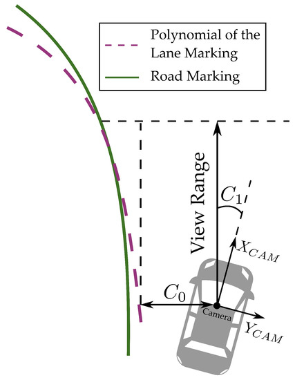
Figure 1.
Illustration of lane marking detection.
These coefficients are explained in Table 1. Since our test scenarios are primarily focused on straight segments of the highway, and are ignored. However, is the lateral distance to the detection lane marking at the height of the camera. indicates the vehicle heading relative to the lane heading and the road markings on the measurement section are symmetrical, implying that values for the left and right lane markings are identical. As a result, this paper will only focus on and estimation, as shown in Figure 1.

Table 1.
Lane detection coefficients from MOBILEYE camera.
Vision-based lane detection is influenced by different factors that contain external environmental parameters [37] (e.g., lane line reflectivity, appearance, and lighting conditions, etc.) as well as vehicle dynamic performance [38] (e.g., speed and heading angle, a departure from the road centerline, etc.), resulting in discrepancies between detection results and the ground truth. This phenomenon can be observed by comparing two different road markings in Figure 1. According to the guide to the expression of uncertainty in measurement, the detection result of the camera can be stated as the best reference quantity plus the measurement uncertainty [39], where uncertainty can be treated as the detection error, and it is estimated by using an NN-based approach in this paper. Finally, a phenomenological camera model is proposed to approximate real-world camera detection performances.
3. Experimental Setup
3.1. Data Collection
The highway was publicly closed during data collection. Lane detection data were collected using the MOBILEYE 630 system installed in the test car. The MOBILEYE camera provides real-time image processing to recognize various road objects such as lane markings, pedestrians, and so on. For this study, the data related to the type of detected longitudinal marking (continuous or dashed), polynomial coefficient of lane marking, and view range were recorded. Meanwhile, the six-degree-of-freedom inertial measurement system of the GENESYS Automotive Dynamic Motion Analyzer (ADMA) for motion analysis is combined with the NOVATEL RTK-GPS receiver to provide a highly accurate vehicle kinematic data. Figure 2 shows the measurement setup used for data collection.
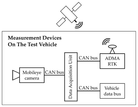
Figure 2.
Measurement setup for measuring vehicle.
3.2. Ground Truth Definition
ADMA-RTK combination is a strap-down inertial measurement system. The extended-Kalman filter used in the ADMA can estimate several important sensor errors in order to enhance system performance. Depending on the capability of the GPS receiver, the position accuracy range down to 1 cm. Meanwhile, six inertial sensors provide high accuracy data [40]. Due to the accurate performance of this combination, it is used as a reference system. The measurements and data collection were conducted on the M86 highway in Hungary, see Figure 3. The construction of a close road section facilitates the development and testing of connected and autonomous vehicles. The total length of the test road section is 3.4 km [41].
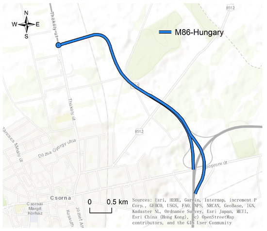
Figure 3.
M86 freeway located near Csorna (Hungary) on route E65 (GNSS coordinates: 47.625778, 17.270162).
In order to perfectly duplicate the real-world test scenario in the simulation environment, the M86 road was converted into an Ultra-High-Definition (UHD) map, a digital twin of reality that accurately represents every detail of the test environment. The production workflow that was applied for the production of the UHD map was presented in [41]. A digital twin-based M86 map was explicitly produced for testing and validating ADAS/AD driving functions with an absolute precision of +/−2 cm as a quality reference source. The extreme high precision of the lane marking data in this map will be used as the ground truth for comparison with the camera detection output. Additionally, this map will also be used for further virtual testing to duplicate simulation results.
4. Methodology
The camera modelling approach and process are presented in Figure 4. The test vehicle collects information from mounted experimental equipment, such as vehicle dynamic data, GPS sensor data and camera data introduced in Section 3. These data will be used for target determination and feature selection. Depending on modelling requirements, sensor detection results contain essential information about the modelling target, which facilitates the calculation of the differences between measured and reference data. This error represents both the camera’s performance and uncertainty in lane detection and the target of the model. In order to improve the performance of the camera model and decrease the training time of NN, data extraction and input features selection are applied, which contribute most to the prediction variable or output used in this case. The selected features based on the ReliefF algorithm are used as input for MLP. The relationships between each input feature and target are evaluated using ReliefF, which is a feature weighting method designed for multi-class, noisy, and incomplete dataset classification issue [42,43]. Once inputs and targets are determined, the MLP-based approach is applied for modelling.
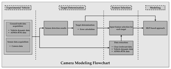
Figure 4.
Schematic representation of necessary components for camera model.
4.1. Target Determination
As previously discussed in Section 2, our model primarily focuses on straight highway segments. Therefore, Lane Position Error (-LPE) and Heading Angel Error (-HAE) are considered as our targets of MLP. Reference data for each target were taken from M86 road marking coordinates and ADMA-RTK reference system, respectively. In addition, detection data for each target were taken from the MOBILEYE camera.
-LPE is calculated as the difference between M86 road markings coordinates and detection data. The calculation process is defined in the next steps:
- Replicating trajectory of GPS data on M86 road map;
- For each timestamp of trajectory data, the test car is positioned on the road, and is calculated for each side of the road, resulting in Left and Right;
- The difference for each side of the road is calculated independently, resulting in -LPE Left and -LPE Right;
- Combining results into a two-dimensional vector provides us with -LPE as the target of MLP.
-HAE is calculated as the difference between the heading angle data provided by the reference system and the detection output of the camera. The calculation is conducted in the same way as mentioned for -LPE, resulting in a one-dimension vector as a target of the MLP. As detailed in the next section, different input features were selected for each target.
4.2. Feature Selection
Various features were collected from different experimental devices and electronic controllers during the measurement process. However, a mass of data often contains many irrelevant or redundant features. In this study, the ADMA reference system provides details on the available data. Some features (ambient temperature, GPS receiver states, altitude, etc.) were discarded because they did not significantly impact vehicle dynamics or camera model functionality. Feature selection aims to maximize information associated with the target, carried out by the extracted features from raw data. Additionally, considering that different features have different update cycles, time synchronization is also required during data processing to align all features on the same timeline. The time synchronization process is as follows:
- The test car’s ADMA-RTK-based trajectory data are selected as a base timeline. Each timestamp from it will be used as a reference point.
- Features will be checked with respect to whether the their timestamp aligns with a reference point within an offset interval from −0.02 s to 0.02 s. They will be saved in a database aligning values with the reference timestamp.
- The process is repeated until it proceeds through all reference points.
In order to further refine and reduce the parameters input to the predictive model, features should be selected from extracted data, which minimizes the number of input features. The benefit of the process is to reduce training time, lower the risk of overfitting, and improve the model’s performance. The primary notions and applications of ReliefF are to rate the quality of features based on their ability in order to distinguish samples that are close to one another. The final weight assigned to each feature is calculated. According to ReliefF results, the final features with the greatest relevance to each target are selected and shown in Table 2, while the corresponding arguments are illustrated in Figure 5. Each set of input chosen features has a defined target. These features are used as inputs to the corresponding MLP model.
Table 2.
Final Feature Selection for each target.
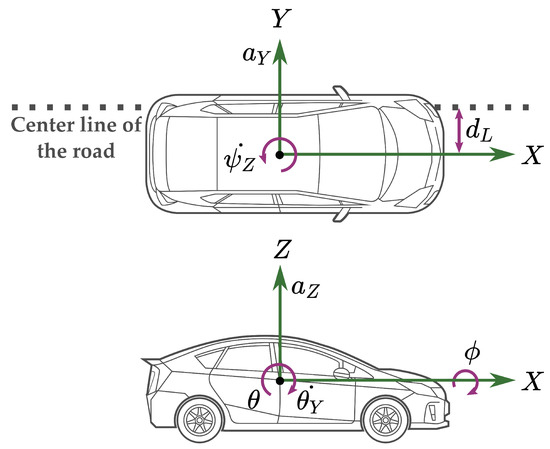
Figure 5.
Illustration of the selected input feature variables on side and top views of the vehicle.
4.3. Neural Network Modelling
MLP is used here to estimate the performance of the camera. It is widely used in different fields, such as system modelling, anomaly detection, and classification applications to solve complex problems in a variety of computer applications [45,46,47,48,49]. Additionally, the MLP approach has been preferred as a method for state estimation and simulation implementation [50]. MLP is useful in research for its ability to solve problems stochastically. Therefore, it is employed here to estimate C0-LPE and C1-HAE.
A typical architecture of MLP has one input layer, one or more hidden layers, and one output layer. The working principle uses the connecting layers, which are components of neurons, to transfer normalized input data to the output. The number of layers in the network and the number of neurons in each layer are typically determined empirically. The architecture of the used MLP is presented in Figure 6. This architecture is used for both prediction models, including the estimation of heading angle and lateral position errors. The data mapping process from input data to the output data is presented in Equations (2)–(4). Furthermore, the arithmetic process in a node is illustrated in Figure 7.
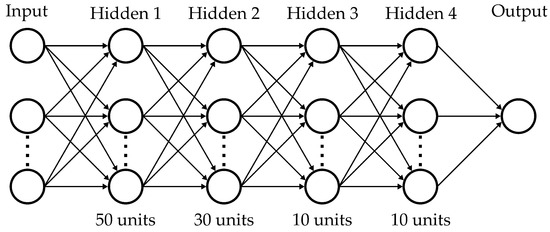
Figure 6.
Proposed MLP architecture.
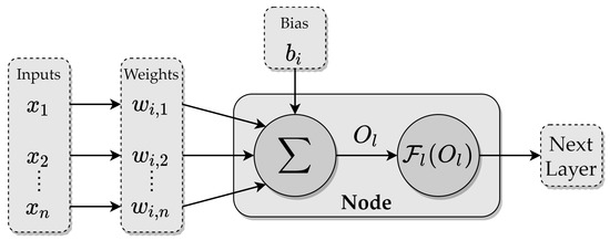
Figure 7.
Data processing in a neural network node.
Each hidden layer contains the associated coefficient weights and bias. The inputs of each node are calculated from the previous layer or are the initial input of the network, then the results of the mathematical operation can be provided by Equation (2), where x is the normalized input variable, w is the weight of each input, i is the input counter, b is the bias of this node, n is the number of input variables, and k and m are the counters of the hidden layer and the number of neural network nodes, respectively.
Subsequently, the results of are applied to function . Here, the hyperbolic tangent sigmoid function is used as an activation function calculated by Equation (3), which defines the output of that node given an input or set of inputs.
Finally, multiple nodes and hidden layers build up the MLP, as shown in the Figure 6. The output of each node is forwarded to the next layer to continue the same operations. The output layer of the entire network is defined by Equation (4), where output calculates the weighted sum of the signals provided by the hidden layer. The coefficients associated with them are grouped into matrices and .
The most critical step in MLP modelling is training. Backpropagation is the most often used training algorithm, which is described as a process for adjusting the network parameters (weights and biases) to minimize the error function between the estimated and real outputs. In comparison to other back-propagation algorithms, a supervised learning algorithm called Scaled Conjugate Gradient (SCG) was selected [51].
The number of layers in the network and the number of neurons in each layer are typically determined empirically. By comparing training result performances, four hidden layers were decided to be utilized in the MLP model, with the number of neurons distributed as 50, 30, 10, and 10 in each layer. The architecture of hidden layers and the number of neurons in each layer are used for both prediction models (-LPE and -HAE estimation). As shown in Section 4.2, the number of inputs for each target is shown in Table 2.
After the definition of the MLP architecture, its performance is evaluated using three different metrics: Mean Squared Error (MSE), Root Mean Square Error (RMSE), and correlation coefficient (R). MSE is used to represent the average squared difference between the estimated values and the actual value (see Equation (5)). On the other hand, RMSE is a typical metric for regression models and is used to quantify the model’s prediction error, with a larger error resulting in a higher value (see Equation (6)). Finally, R represents the proportion of real output dynamics that could be caught by the MLP model. R varies between 0 and 1. A higher number indicates that the model is more accurate in its predictions (see Equation (7)).
5. Results and Discussion
Real-world collected road test data are utilized to train the network model in order to evaluate the accuracy of PLDM better. This section explains MLP training results. Moreover, in order to verify the accuracy of model predictions and the validity of the approach, the employed MLP model results are compared with five other algorithms. Finally, this model will be deployed in the vehicle simulation software CarMaker from IPG Automotive GmbH [52].
5.1. Training Results
In order to train the MLP model, the data gathered by the various devices are synchronized, and 9010 samples were selected from collected data to optimize the model. Input data are randomly separated into three sets: training (70%), validation (15%), and test (15%). The configuration of the MLP model is discussed in Section 4.3 and presented in Table 3. Supervised training is performed on the model using the training set. The validation set is also used to mitigate the issue of overfitting. Finally, the test set is used to evaluate model performance on unseen data.
Table 3.
MLP network model configuration for and estimation.
As discussed in Section 4.1 and Section 4.2, the MLP model is used to estimate -LPE, which consists of five features and a two-dimension target. The combination of five input features and a one-dimension target is used to estimate -HAE. The regression graphs obtained as results of the MLP training are given in Figure 8. The models are evaluated for the test set after convergence, and regression accuracy can achieve 94.0% and 95.5%, respectively, for -LPE and -HAE estimation in order to further evaluate the estimation model, where evaluation metrics (MSE, RMSE, and R) measure regression performance. As a result, MLP training performance is provided in Table 4. The results show good agreement between actual and estimated values, and the prediction errors of the results are within an acceptable range. The models are more consistent with the trend of real values in terms of the predicted value. Therefore, the training of the network has been successfully provided.
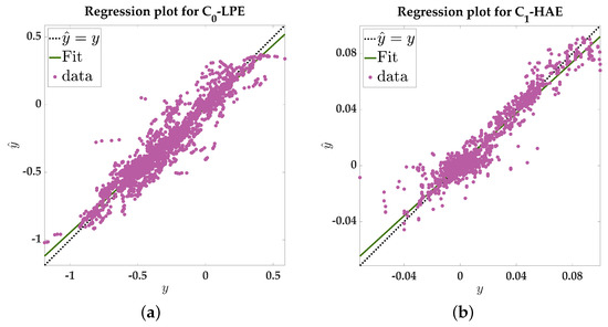
Figure 8.
MLP training regression graph. (a) Training regression result for -LPE (b) Training regression result for -HAE.
Table 4.
Performance evaluation of MLP for -LPE and -HAE estimation.
5.2. Comparing with Other Approaches
The proposed method can be used for -LPE and -HAE predictions and for comparing the effectiveness and accuracy of this method. Moreover, five other machine learning methods are introduced in [53,54], and these algorithms are categorized and introduced as follows:
- Support Vector Machine (SVM): It is a widely utilized soft computing method in various fields. The fundamental idea is to fit data in specific areas by using non-linear mappings and to apply linear methods in function space, which has been applied for a regression problem and demonstrates superior generalization performance [55].
- Linear Regression (LR): It attempts to model the connection between two variables by fitting a linear equation to the observed data. One is the explanatory variable, and the other is the dependent variable. This algorithm is a fundamental regression method introduced in [56].
- Gaussian Regression of Process (GPR): It combines the structural properties of Bayesian NN with the nonparametric flexibility of Gaussian processes [57]. This model considers the input-dependent signal and noise correlations between various response variables. It performs well on small datasets and can also be used to measure prediction uncertainty.
- Ensemble Boosting (EB): The idea of an EB is presented in [58], and it fits a wide range of regression problems, and the architecture is the generation of sequential hypotheses, where each hypothesis tries to improve the previous one. General bias errors are eliminated throughout the sequencing process, and good predictive models are generated.
- Stepwise regression (SR): It is the iterative process of building a regression model by selecting independent variables to be used in a final model, which is introduced and applied in [59]. It entails gradually increasing or decreasing the number of putative explanatory factors and evaluating statistical significance after each cycle.
Finally, these five algorithms and MLP model are compared with performance metrics, as shown in Table 5. In comparison, the suggested MLP achieves outstanding results while outperforming alternative approaches. Additionally, the GPR demonstrated a rather good regression result, with an accuracy of 83% and 86% for -LPE and -HAE estimation, respectively; this is probably because the GPR kernel can extract sequential data from complex temporal structures. All three models, SVM, LR, and SR showed comparable performance and underfitting for -LPE. Furthermore, two other neural network models based on data-driven approaches are introduced in [23,24], which include Mixture Density Network (MDN) and deep Gaussian Process (GP). MDN outputs a Gaussian mixture through a multilayer perceptron. Each Gaussian distribution is assigned a corresponding weight, which predicts the entire probability distribution. Deep GP is a deep belief network based on GP mappings. The data are modelled as the outputs of a multivariate GP. Both models can accurately represent uncertainty between camera detection and measurement results, but they do not produce an accurate estimate compared to MLP. Therefore, driven by the goal of the digital twin, MLP can more accurately represent the behaviour of sensors in real environments and still show substantial advantages.
Table 5.
Performance comparison between several regression algorithms.
5.3. Virtual Validation in CarMaker
In this section, a test run is randomly selected from the test set samples carried out in the co-simulation based on the Carmaker-Simulink software, which provides a multi-body simulation environment that includes vehicle dynamics control and sensor modules. These modules can support custom modifications. Thus, PLDM replaces the default camera model in CarMaker and tests detection performance in a virtual environment. As illustrated in Figure 9, the entire model is integrated into the co-simulation platform. Realistic reproduction of the virtual scenario is produced using the digital twin-based M86 map. Subsequently, at each time step, the ideal CarMaker object sensor detects the object from the map and provides precise information feedback in list format. In particular, test run data from previous tests conducted in a real-world environment, such as vehicle dynamics and positioning information, are stored in an external file that could be utilized as input for free movement in CarMaker. This module is mainly responsible for real measurement playback, and necessary data are transmitted to the MLP-based error estimation module, where the estimator predicts the corresponding error values for -LPE and -HAE, respectively, based on the current vehicle state. Due to the fact that the MLP model was trained on prior training data successfully, ground-truth lane marking data are manipulated according to the model’s output. In this case, two polynomial coefficients (-LPE and -HAE) of lane marking detection can be determined.
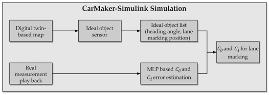
Figure 9.
The procedure of the phenomenological lane detection model in simulation.
As shown in Figure 10, the estimated value and real value of the randomly selected samples are generally consistent with the trend of the sample change. Affected by real factors, the method to make predictions for certain samples still contains certain errors. A larger of the left lane estimation error greater than the right lane estimation can be observed, probably because the left lane line is dashed and the right lane line is continuously solid. Namely, a dashed lane marking is usually more challenging to determine from the background in a captured image, as explained in [60]. Overall, the predicted peak and valley space corresponding to the estimated values still contains some errors compared to the actual values. However, the maximum error value of 0.05 m is still acceptable. The reason is that this method takes into account many more factors than traditional regression forecasting methods, and it is hard to avoid errors in the weights of some secondary factors. However, in terms of the overall trend, the effectiveness of the chosen model is proven.
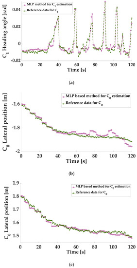
Figure 10.
Simulation result for and estimation. (a) estimation comparison between camera detection data and MLP based output. (b) of left lane estimation comparison between camera detection data and MLP based output. (c) of right lane estimation comparison between camera detection data and MLP-based output.
6. Conclusions
In order to support efficient virtual test and validation of LKA systems, this study developed an MLP model to determine lane detection -LPE and -HAE estimation based on the relationship of vehicle dynamic data. This relationship is complex for an actual dataset derived from real-world measurements and requires an artificial intelligence method to create a reliable model to analyze the problem. This approach was divided into three parts. Firstly, the measurements and data collection were carried out for the testing procedure, and digital twin-based data were defined as ground truth. The second part was to extract data and select features from the actual collected data to find input data that had greater influences on the model, thus improving training efficiency. In the third part of the study, an MLP model was developed, and the selected features were used as inputs to train the model. The results also showed that MLP can produce higher accuracy than other regression approaches. Finally, the technique was employed to reproduce lane detection behaviour of an automotive camera system in a simulation platform. Combined with the analysis of the simulation results, we found that the best regression is achieved for a given non-linear dataset. Due to the fact that existing data and tests were conducted primarily on straight roads, lane marking detection on curved roads will be taken into account to refine the model further and improve our approach.
The model fits the detection error of the sensor output by using selected features, which enables fast and efficient sensor modelling. Compared to the physical model, this approach simplifies the modelling process by ignoring physical performance modelling of the camera components as well as the perception algorithm and focusing only on the inputs and outputs of the camera system, thus improving computational performance. Moreover, in contrast to the ideal models previously mentioned, ideal sensor models provide only ground truth information without any specific post-processing function. Therefore, physical effects do not influence these models. However, PLDM models based on the MLP approach can provide more details about sensor detection performance than an ideal model, enhancing the simulation’s realism. Although there is a strong correlation between modelling complexity, training time, data composition and volume, modelling efficiency is improved, and this approach is generic. It can be applied to various sensors with low efforts after initial development.
Author Contributions
Conceptualization, H.L.; methodology, H.L. and S.A.; software, H.L. and K.T.; validation, H.L. and K.T.; investigation, H.L.; resources, D.B. (Darko Babic), D.B. (Dario Babic), Z.F.M. and V.T.; data curation, H.L., K.T. and C.W.; writing—original draft preparation, H.L. and K.T.; writing—review and editing, H.L., S.A. and A.E.; visualization, H.L.; supervision, A.E. and M.C.B. All authors have read and agreed to the published version of the manuscript.
Funding
Open Access Funding by the Graz University of Technology.
Data Availability Statement
Not applicable.
Acknowledgments
The author thanks those who have supported this research, to the Graz University of Technology also.
Conflicts of Interest
The authors declare no conflict of interest.
References
- Administration, N.H.T.S. National motor vehicle crash causation survey: Report to congress. Natl. Highw. Traffic Saf. 2008, 811, 059. [Google Scholar]
- Cicchino, J.B. Effects of lane departure warning on police-reported crash rates. J. Saf. Res. 2018, 66, 61–70. [Google Scholar] [CrossRef] [PubMed]
- Eichberger, A.; Rohm, R.; Hirschberg, W.; Tomasch, E.; Steffan, H. RCS-TUG Study: Benefit potential investigation of traffic safety systems with respect to different vehicle categories. In Proceedings of the 24th International Technical Conference on the Enhanced Safety of Vehicles (ESV), Washington, DC, USA, 8–11 June 2011. [Google Scholar]
- Jianwei, N.; Jie, L.; Mingliang, X.; Pei, L.; Zhao, X. Robust Lane Detection Using Two-stage Feature Extraction with Curve Fitting. Pattern Recognit. 2016, 59, 225–233. [Google Scholar]
- Aly, M. Real time detection of lane markers in urban streets. In 2008 IEEE Intelligent Vehicles Symposium; IEEE: Piscataway, NJ, USA, 2008; pp. 7–12. [Google Scholar]
- Zhang, Y.; Lu, Z.; Zhang, X.; Xue, J.H.; Liao, Q. Deep Learning in Lane Marking Detection: A Survey. IEEE Trans. Intell. Transp. Syst. 2021. [Google Scholar] [CrossRef]
- Wang, Z.; Ren, W.; Qiu, Q. Lanenet: Real-time lane detection networks for autonomous driving. arXiv 2018, arXiv:1807.01726. [Google Scholar]
- Cireşan, D.C.; Giusti, A.; Gambardella, L.M.; Schmidhuber, J. Mitosis detection in breast cancer histology images with deep neural networks. In Proceedings of the International Conference on Medical Image Computing and Computer-Assisted Intervention, Nagoya, Japan, 22–26 September 2013; pp. 411–418. [Google Scholar]
- Chng, Z.M.; Lew, J.M.H.; Lee, J.A. RONELD: Robust Neural Network Output Enhancement for Active Lane Detection. In Proceedings of the 2020 25th International Conference on Pattern Recognition (ICPR), Milan, Italy, 10–15 January 2021; pp. 6842–6849. [Google Scholar]
- Kim, J.; Lee, M. Robust lane detection based on convolutional neural network and random sample consensus. In Proceedings of the International Conference on Neural Information Processing, Montreal, QC, Canada, 8–13 December 2014; pp. 454–461. [Google Scholar]
- Kalra, N.; Paddock, S.M. Driving to safety: How many miles of driving would it take to demonstrate autonomous vehicle reliability? Transp. Res. Part A Policy Pract. 2016, 94, 182–193. [Google Scholar] [CrossRef]
- Shladover, S.E. Connected and automated vehicle systems: Introduction and overview. J. Intell. Transp. Syst. 2018, 22, 190–200. [Google Scholar] [CrossRef]
- Hussain, R.; Zeadally, S. Autonomous cars: Research results, issues, and future challenges. IEEE Commun. Surv. Tutorials 2018, 21, 1275–1313. [Google Scholar] [CrossRef]
- Bardt, H. Autonomous Driving—A Challenge for the Automotive Industry. Intereconomics 2017, 52, 171–177. [Google Scholar] [CrossRef][Green Version]
- Bellem, H.; Klüver, M.; Schrauf, M.; Schöner, H.P.; Hecht, H.; Krems, J.F. Can we study autonomous driving comfort in moving-base driving simulators? A validation study. Hum. Factors 2017, 59, 442–456. [Google Scholar] [CrossRef]
- Uricár, M.; Hurych, D.; Krizek, P.; Yogamani, S. Challenges in designing datasets and validation for autonomous driving. arXiv 2019, arXiv:1901.09270. [Google Scholar]
- Li, W.; Pan, C.; Zhang, R.; Ren, J.; Ma, Y.; Fang, J.; Yan, F.; Geng, Q.; Huang, X.; Gong, H.; et al. AADS: Augmented autonomous driving simulation using data-driven algorithms. Sci. Robot. 2019, 4. [Google Scholar] [CrossRef] [PubMed]
- Schlager, B.; Muckenhuber, S.; Schmidt, S.; Holzer, H.; Rott, R.; Maier, F.M.; Saad, K.; Kirchengast, M.; Stettinger, G.; Watzenig, D.; et al. State-of-the-Art Sensor Models for Virtual Testing of Advanced Driver Assistance Systems/Autonomous Driving Functions. SAE Int. J. Connect. Autom. Veh. 2020, 3, 233–261. [Google Scholar] [CrossRef]
- Stolz, M.; Nestlinger, G. Fast generic sensor models for testing highly automated vehicles in simulation. EI 2018, 135, 365–369. [Google Scholar] [CrossRef]
- Muckenhuber, S.; Holzer, H.; Rübsam, J.; Stettinger, G. Object-based sensor model for virtual testing of ADAS/AD functions. In Proceedings of the 2019 IEEE International Conference on Connected Vehicles and Expo (ICCVE), Graz, Austria, 4–8 November 2019; pp. 1–6. [Google Scholar]
- Hanke, T.; Hirsenkorn, N.; Dehlink, B.; Rauch, A.; Rasshofer, R.; Biebl, E. Generic architecture for simulation of ADAS sensors. In Proceedings of the 2015 16th International Radar Symposium (IRS), Dresden, Germany, 24–26 June 2016; pp. 125–130. [Google Scholar]
- Genser, S.; Muckenhuber, S.; Solmaz, S.; Reckenzaun, J. Development and Experimental Validation of an Intelligent Camera Model for Automated Driving. Sensors 2021, 21, 7583. [Google Scholar] [CrossRef]
- Yang, T.; Li, Y.; Ruichek, Y.; Yan, Z. Performance Modeling a Near-Infrared ToF LiDAR Under Fog: A Data-Driven Approach. IEEE Trans. Intell. Transp. Syst. 2021. [Google Scholar] [CrossRef]
- Fang, W.; Zhang, S.; Huang, H.; Dang, S.; Huang, Z.; Li, W.; Wang, Z.; Sun, T.; Li, H. Learn to Make Decision with Small Data for Autonomous Driving: Deep Gaussian Process and Feedback Control. J. Adv. Transp. 2020, 2020, 8495264. [Google Scholar] [CrossRef]
- Hanke, T.; Hirsenkorn, N.; Dehlink, B.; Rauch, A.; Rasshofer, R.; Biebl, E. Classification of sensor errors for the statistical simulation of environmental perception in automated driving systems. In Proceedings of the 2016 IEEE 19th International Conference on Intelligent Transportation Systems (ITSC), Rio de Janeiro, Brazil, 1–4 November 2016; pp. 643–648. [Google Scholar]
- Hirsenkorn, N.; Hanke, T.; Rauch, A.; Dehlink, B.; Rasshofer, R.; Biebl, E. A non-parametric approach for modeling sensor behavior. In Proceedings of the 2015 16th International Radar Symposium (IRS), Dresden, Germany, 24–26 June 2015; pp. 131–136. [Google Scholar]
- Eder, T.; Hachicha, R.; Sellami, H.; van Driesten, C.; Biebl, E. Data Driven Radar Detection Models: A Comparison of Artificial Neural Networks and Non Parametric Density Estimators on Synthetically Generated Radar Data. In Proceedings of the 2019 Kleinheubach Conference, Miltenberg, Germany, 23–25 September 2019; pp. 1–4. [Google Scholar]
- Höber, M.; Nalic, D.; Eichberger, A.; Samiee, S.; Magosi, Z.; Payerl, C. Phenomenological Modelling of Lane Detection Sensors for Validating Performance of Lane Keeping Assist Systems. In Proceedings of the 2020 IEEE Intelligent Vehicles Symposium (IV), Las Vegas, NV, USA, 23 June 2020; pp. 899–905. [Google Scholar]
- Schneider, S.A.; Saad, K. Camera Behavior Models for ADAS and AD functions with Open Simulation Interface and Functional Mockup Interface. Cent. Model Based Cyber Phys. Prod. Dev. 2018, 20, 19-19. [Google Scholar]
- Schneider, S.A.; Saad, K. Camera behavioral model and testbed setups for image-based ADAS functions. EI 2018, 135, 328–334. [Google Scholar] [CrossRef]
- Wittpahl, C.; Zakour, H.B.; Lehmann, M.; Braun, A. Realistic image degradation with measured PSF. Electron. Imaging 2018, 2018, 149-1. [Google Scholar] [CrossRef]
- Carlson, A.; Skinner, K.A.; Vasudevan, R.; Johnson-Roberson, M. Modeling camera effects to improve visual learning from synthetic data. In Proceedings of the European Conference on Computer Vision (ECCV) Workshops, Munich, Germany, 8–14 September 2018. [Google Scholar]
- Eichberger, A.; Markovic, G.; Magosi, Z.; Rogic, B.; Lex, C.; Samiee, S. A Car2X sensor model for virtual development of automated driving. Int. J. Adv. Robot. Syst. 2017, 14, 1729881417725625. [Google Scholar] [CrossRef]
- Bernsteiner, S.; Magosi, Z.; Lindvai-Soos, D.; Eichberger, A. Radarsensormodell für den virtuellen Entwicklungsprozess. ATZelektronik 2015, 10, 72–79. [Google Scholar] [CrossRef]
- Ponn, T.; Müller, F.; Diermeyer, F. Systematic analysis of the sensor coverage of automated vehicles using phenomenological sensor models. In Proceedings of the 2019 IEEE Intelligent Vehicles Symposium (IV), Paris, France, 9–12 June 2019; pp. 1000–1006. [Google Scholar]
- Mobileye. LKA Common CAN Protocol; Mobileye: Jerusalem, Israel, 2019. [Google Scholar]
- Borkar, A.; Hayes, M.; Smith, M.T.; Pankanti, S. A layered approach to robust lane detection at night. In Proceedings of the 2009 IEEE Workshop on Computational Intelligence in Vehicles and Vehicular Systems, Nashville, TN, USA, 30 March–2 April 2009; pp. 51–57. [Google Scholar]
- Li, Y.; Zhang, W.; Ji, X.; Ren, C.; Wu, J. Research on lane a compensation method based on multi-sensor fusion. Sensors 2019, 19, 1584. [Google Scholar] [CrossRef]
- BIPM; IEC; ISO; IUPAC; IUPAP; OML. Guide to the Expression of Uncertainty in Measurement; BIPM: Tokyo, Japan, 1995. [Google Scholar]
- Schneider, D.; Schick, B.; Huber, B.; Lategahn, H. Measuring Method for Function and Quality of Automated Lateral Control Based on High-precision Digital Grund Truth Maps. In VDI/VW-Gemeinschaftstagung Fahrerassistenzsysteme und Automatisiertes Fahren 2018; VDI: Düsseldorf, Germany, 2018; pp. 3–15. [Google Scholar]
- Tihanyi, V.; Tettamanti, T.; Csonthó, M.; Eichberger, A.; Ficzere, D.; Gangel, K.; Hörmann, L.B.; Klaffenböck, M.A.; Knauder, C.; Luley, P. Motorway measurement campaign to support R&D activities in the field of automated driving technologies. Sensors 2021, 21, 2169. [Google Scholar] [PubMed]
- Zhang, J.; Chen, M.; Zhao, S.; Hu, S.; Shi, Z.; Cao, Y. ReliefF-based EEG sensor selection methods for emotion recognition. Sensors 2016, 16, 1558. [Google Scholar] [CrossRef] [PubMed]
- Palma-Mendoza, R.J.; Rodriguez, D.; De-Marcos, L. Distributed ReliefF-based feature selection in Spark. Knowl. Inf. Syst. 2018, 57, 1–20. [Google Scholar] [CrossRef]
- GmbH, G.E. Technical Documentation ADMA Version 1.0; GeneSys Electronik GmbH: Offenburg, Germany, 2013. [Google Scholar]
- Khatib, T.; Mohamed, A.; Sopian, K.; Mahmoud, M. Estimating ambient temperature for Malaysia using generalized regression neural network. Int. J. Green Energy 2012, 9, 195–201. [Google Scholar] [CrossRef]
- Lee, D.; Yeo, H. A study on the rear-end collision warning system by considering different perception-reaction time using multi-layer perceptron neural network. In Proceedings of the 2015 IEEE Intelligent Vehicles Symposium (IV), Seoul, Korea, 28 June–1 July 2015; pp. 24–30. [Google Scholar]
- Liu, B.; Zhao, Q.; Jin, Y.; Shen, J.; Li, C. Application of combined model of stepwise regression analysis and artificial neural network in data calibration of miniature air quality detector. Sci. Rep. 2021, 11, 1–12. [Google Scholar]
- Bishop, C.M.; Roach, C. Fast curve fitting using neural networks. Rev. Sci. Instruments 1992, 63, 4450–4456. [Google Scholar] [CrossRef]
- Li, Y.; Tang, G.; Du, J.; Zhou, N.; Zhao, Y.; Wu, T. Multilayer perceptron method to estimate real-world fuel consumption rate of light duty vehicles. IEEE Access 2019, 7, 63395–63402. [Google Scholar] [CrossRef]
- Ceven, S.; Bayir, R. Implementation of Hardware-in-the-Loop Based Platform for Real-time Battery State of Charge Estimation on Li-Ion Batteries of Electric Vehicles using Multilayer Perceptron. Int. J. Intell. Syst. Appl. Eng. 2020, 8, 195–205. [Google Scholar] [CrossRef]
- Møller, M.F. A scaled conjugate gradient algorithm for fast supervised learning. Neural Netw. 1993, 6, 525–533. [Google Scholar] [CrossRef]
- IPG CarMaker. Reference Manual (V 8.1.1).; IPG Automotive GmbH: Karlsruhe, Germany, 2019. [Google Scholar]
- Chandran, V.; Patil, C.K.; Karthick, A.; Ganeshaperumal, D.; Rahim, R.; Ghosh, A. State of charge estimation of lithium-ion battery for electric vehicles using machine learning algorithms. World Electr. Veh. J. 2021, 12, 38. [Google Scholar] [CrossRef]
- Liao, X.; Li, Q.; Yang, X.; Zhang, W.; Li, W. Multiobjective optimization for crash safety design of vehicles using stepwise regression model. Struct. Multidiscip. Optim. 2008, 35, 561–569. [Google Scholar] [CrossRef]
- Cherkassky, V.; Ma, Y. Practical selection of SVM parameters and noise estimation for SVM regression. Neural Netw. 2004, 17, 113–126. [Google Scholar] [CrossRef]
- Montgomery, D.C.; Peck, E.A.; Vining, G.G. Introduction to Linear Regression Analysis; John Wiley & Sons: Hoboken, NJ, USA, 2021. [Google Scholar]
- Quinonero-Candela, J.; Rasmussen, C.E. A unifying view of sparse approximate Gaussian process regression. J. Mach. Learn. Res. 2005, 6, 1939–1959. [Google Scholar]
- Avnimelech, R.; Intrator, N. Boosting regression estimators. Neural Comput. 1999, 11, 499–520. [Google Scholar] [CrossRef]
- Zhou, N.; Pierre, J.W.; Trudnowski, D. A stepwise regression method for estimating dominant electromechanical modes. IEEE Trans. Power Syst. 2011, 27, 1051–1059. [Google Scholar] [CrossRef]
- Hoang, T.M.; Hong, H.G.; Vokhidov, H.; Park, K.R. Road lane detection by discriminating dashed and solid road lanes using a visible light camera sensor. Sensors 2016, 16, 1313. [Google Scholar] [CrossRef]
Publisher’s Note: MDPI stays neutral with regard to jurisdictional claims in published maps and institutional affiliations. |
© 2021 by the authors. Licensee MDPI, Basel, Switzerland. This article is an open access article distributed under the terms and conditions of the Creative Commons Attribution (CC BY) license (https://creativecommons.org/licenses/by/4.0/).