Abstract
This paper proposes enhanced prediction and control design methods for improving traffic flow with human-driven and automated vehicles. To achieve accurate prediction for the entire time horizon, data-driven and model-based prediction methods were integrated. The goal of the integration was to accurately predict the outflow of the traffic network, which was selected as the highway section in this paper. The proposed novel prediction method was used in the optimal design for calculating controlled inflows on highway ramps. The goal of the design was to reach the maximum outflow of the traffic network, even against disturbances on uncontrolled inflows of the network. The control design leads to an optimization problem based on the min–max principle, i.e., the traffic outflow is considered to be maximized by controlled inflows and to be minimized by uncontrolled inflows. The effectiveness of the prediction and the control methods through simulation examples are illustrated, i.e., traffic outflow can be maximized by the control system under various uncontrolled inflow values.
1. Introduction and Motivation
Providing control strategies for automated vehicles has become a subject of significant focus in research and development centers of vehicle industry. An important task is to design a velocity profile for vehicles in order to guarantee effective, comfortable, safe and economical traffic by exploiting vehicle dynamics and environmental circumstances, e.g., certain characteristics of fuel consumption, delivered cargo, road inclinations, speed limits, traffic flow and traffic forecast. The complexity of the control task results in various performance requirements which must be simultaneously guaranteed by the control system [].
Existing control solutions result in speed profiles for automated vehicles, which differ from the speed selection strategy of human drivers. The reason for this is that the control systems of automated vehicles can obtain information on the road ahead, e.g., the usage of the road capacity or the upcoming downhill terrain characteristics. At the same time, most of these data are not available for human drivers. It can be shown that the speed selection of automated vehicles and human-driven vehicles are not independent from each other. Consequently, the motion of human-driven vehicles must be adapted to automated vehicles. Moreover, the ratio of automated vehicles () in the entire traffic network also influences the characteristics of the traffic flow through the modification of traffic speed.
1.1. Motivation Example on the Variation of Traffic Flow
Figure 1 presents an illustration of the impact of on the variation in average traffic speed. In this scenario, a 20 km-long three-lane (outer, middle and inner lanes) segment of the hilly Hungarian M1 highway is modeled in a VISSIM traffic simulator. In the simulation scenario, the speed limit is 130 km/h, except for the section between 6 and 8 km, where the speed limit is 90 km/h. Without automated vehicles , the average traffic speed is close to the speed limit, as can be seen in Figure 1a. When there is an increased number of automated vehicles on the highway , the average traffic speed varies due to the automated vehicles, whose speed profiles are also influenced by the uphill and downhill sections. The latter case results in an approximately decrease in energy consumption, within the entire traffic, compared to the previous case, i.e., without automated vehicles.
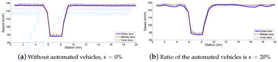
Figure 1.
Average traffic speed of the traffic in the example.
Figure 2 shows further examinations of the traffic flow in the distinct segments of the highway. q denotes the inflow of the motorway (veh/h). Figure 2a,b show the results of the scenario in the cases of the previous example, i.e., and , respectively. In these examples, the inflow into the highway section is veh/h. Figure 2c presents the result of the scenario, in which the ratio of automated vehicles is . Moreover, Figure 2d presents the result of the scenario, in which the inflow into the highway section is significantly increased to veh/h, and . Through the illustrations, it can be concluded that increasing the ratio and/or increasing the inflow has a significant impact on traffic flow.
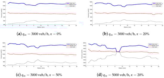
Figure 2.
Illustration of the traffic flow depending on the inflow and the ratio of automated vehicles.
1.2. Brief Literature Overview on the Related Achievements
Since automated vehicles have a significant impact on traffic flow, it is necessary to take the modeling and control design of the traffic system into consideration. A comprehensive overview of different classical control solutions for ramp metering has been proposed by [,]. Moreover, the vehicle-to-infrastructure (V2I) communication provides new perspectives in the control of the traffic system, because a huge amount of data about the motion of the vehicles in the traffic network can be obtained []. This allows a more sophisticated prediction of the upcoming traffic scenario, in which the effectiveness of the traffic control can be improved.
The exploitation of the result of the traffic flow analysis in the modeling and control of automated vehicles is one of the hot topics among researchers, as can be seen in (e.g., []). The most important approaches of traffic flow modeling were summarized by []. The analysis of the traffic flow, in which semi-automated and automated vehicles travel alongside human-driven vehicles, was proposed by []. Stability issues of the traffic flow of connected and automated vehicles were examined by []. In [], it has been shown that automated vehicles have only slightly negative effects but significant positive effects on the traffic flow depending on the penetration rate of the automated vehicles and the traffic scenario. Interactions between automated and human-driven vehicles were presented in []. The authors in [] highlighted new achievements in the construction of a macroscopic fundamental diagram for traffic flow with automated vehicles. The presented data analysis results revealed that the traditional triangular fundamental diagram structure remains applicable to describe the traffic flow characteristics of traffic with automated vehicles. For mixed traffic, a parsimonious formula was provided to estimate the fundamental diagram with measures from pure human-driven traffic and pure automated vehicle traffic. Control-oriented applications are strongly connected to the modeling of traffic flow. For example, in [], a network-level coordination for automated vehicle control and traffic light control was presented, i.e., a distributed optimization scheme to reduce the computational complexity and to improve the effectiveness of coordination was developed. A more complex problem was that of control in mixed traffic, because the motion of automated vehicles and the motion of human-driven vehicles simultaneously impact the traffic flow. The interactions between human-driven and autonomous vehicles in optimal control synthesis for tolls were studied by [].
Based on the huge amount of data on traffic, a novel data-driven approach for the analysis and modeling of traffic flow dynamics was proposed by []. Traffic flow prediction using a deep-learning algorithm was presented by []. In that study, a deep-learning architecture model was applied by using auto-encoders as building blocks to represent traffic flow features for prediction. Similarly, Lasso regression was used for traffic flow prediction in []. Cell phone information-based big data analysis and control for transportation purposes was proposed by []. The work of [] focused on generating models for microscopic traffic simulation, which was built upon real-world data. The identification and prediction of traffic flow states based on the big data analysis method was presented by []. An increased number of achievable information on traffic flow was used for training deep neural networks, which were then able to predict traffic flow under urban traffic scenarios, as can be seen in []. A deep learning method using convolutional neural network and long short-term memory architectures for monitoring traffic flow in urban region was provided by []. The fusion-based technique resulted in high accuracy based on the evaluation through simulation scenarios.
1.3. Proposed Methodology of the Paper
The overview of the literature shows that several approaches exist for modeling traffic flow dynamics, but most of these are related to pure human-driven or automated vehicles. The modeling and analysis of mixed traffic flow is an emerging research field, in which partial solutions have been achieved. Modeling methods with classical model-based approaches do exist [], as do those with unconventional, e.g., network-level [] or data-driven approaches []. Methodologically, the classical traffic modeling methods are based on physical relationships, in which the nonlinear characteristics of the traffic flow are described. The advantage of these methods is that the traffic flow model provides theoretical fundamentals for designing a controller with guaranteed performances []. Nevertheless, their drawback is the increased uncertainty concerning the modeling of short-time traffic flow, due to robustness features. In the case of data-driven modeling methods, the actual measured information on the traffic flow is highly relevant, i.e., the short-time prediction of forthcoming traffic flow can be more accurate due to the actual information. However, the data-driven modeling solutions also have disadvantages. In the case of neural-network-based formulation, the evaluation of the prediction/control process is challenging, while in the case of a regression-based formulation, the accuracy of long-time prediction can be limited.
In spite of the various existing methods, it is difficult to find a systematic control-oriented modeling method which exploits the advantages of data-driven analysis. The aim of this paper was to integrate data-driven traffic flow prediction in a polynomial model-based traffic flow model and thus, improve the accuracy of the prediction. The proposed novel prediction method for control design purposes was applied, i.e., an optimization problem of traffic flow volume with a ramp metering by the min–max principle was provided. The resulting control system provides robustness against disturbances of the system, i.e., the uncontrolled inflows of the traffic network. A novel contribution of this paper is that the proposed prediction model is able to handle the presence of automated vehicles in the traffic network at the level of data-driven prediction as well as at the level of the polynomial traffic flow model.
The prediction and control process is illustrated in Figure 3. The proposed prediction method has two components, namely data-driven prediction and model-based prediction. Their outputs are the predicted flow volumes at the end of the highway section on a horizon. The outputs of the predictions were integrated into a final prediction , which is used in the control process. The output of the control comprises the controlled inflows on N number of ramps on horizon . The control inputs on the entire horizon are used in the prediction process and their values at the step are used as control inputs of the traffic network. Different measurements on the traffic network for each prediction block are used as inputs and thus, the control loop is closed.
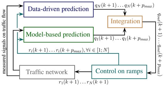
Figure 3.
Illustration of the prediction and control process.
The paper is organized as follows. In Section 2, the data-driven estimation of the traffic flow is presented. This is performed through a two-step analysis. First, a subset selection method is applied, which is able to prioritize the main attributes based on their relations to the measured signals. Second, a linear regression model using the least squares (LS) method is applied to derive a relationship between the attributes and the traffic flow. Section 3 proposes an enhanced traffic flow model, which results from the interconnection of the data-driven prediction and the classical traffic flow modeling. Section 4 proposes the traffic flow control. The effectiveness of the novel optimal control is demonstrated through simulation scenarios. In this paper, the VISSIM complex traffic simulator was used the modeling and simulation of the traffic network, while the WEKA data-mining software was used in the LS-based analysis, as can be seen in []. Finally, Section 6 summarizes with some concluding remarks.
2. Data-Driven Prediction of the Traffic Flow
In this section, data-driven analysis for the prediction of traffic flow dynamics is proposed. The purpose is to find a mathematical structure, which can be used to model the real-time prediction of the forthcoming traffic flow values.
2.1. Brief Overview of Data-Driven Analysis
In this paper, LS-based estimation with subset selection was used to generate prediction models for the traffic flow. In the following, the most important features, based on the work of [], are briefly summarized.
The difficulty in data-driven estimation is that a model should be obtained from a large number of measurements. Consider a dataset with n independent instances, b input variables and one output variable. The instances are written in the form of dimension design matrix X. Let be the parameter vector of the true prediction model . Through the application of X and , the resulting output vector y is determined as
where is the noise vector, whose elements have normal distribution with variance. It is assumed that is known or can be estimated, which is denoted by .
If the number of inputs b of the model increases, the number of subset models also increases by , which may lead to a computationally unfeasible LS estimation task. Therefore, the effective estimation requires the determination of preferences among the sets of variables in . The subset selection is based on the instances X, whose subset models are generated. In the generation of subset models, it is necessary to reduce the complexity of the estimation problem, while information loss from the data must be limited [].
The goal of the subset selection is to find the attributes of , which have a significant impact on y. Consider instance i from vector y as
where values are the elements of vector . For the selection of the relevant subsets, it is necessary to analyze the sensitivity of depending on . Since the attributes are time-domain variables, the partial derivatives of (2) are computed as
The partial derivatives are computed for all n instances using the measured signals (3). This results in n number of derivatives for all attributes. If the deviation of the resulting partial derivatives for a given attribute is small, then it has a significant impact on y. This attribute is incorporated in the prediction model and is estimated with high effectiveness. However, if the deviation of the resulting values is high, then attribute j may not be part of the prediction model.
The decision to incorporate j into the prediction model was made based on the probability density function, which is fitted in a Gaussian form:
where and are the mean and the deviation of , respectively. The relevance of an attribute can be expressed by integrating the Gaussian function and taking into account the sign of together with the scaling of as
where expresses the relevance of an attribute on y. In the subset selection, it is necessary to compute its value for all attributes b. In the selection procedure, the values of are arranged in descending order and the first l number of attributes is selected for taking part in the prediction model. l is a previously defined scalar value, which is required to select as small as possible values to result in a relatively simple prediction model for real-time computation.
In the next step, the coefficients of the linear prediction model was computed. The prediction was formed as
where contains the coefficients of the attributes and is an dimension subset of matrix X. The purpose of selection is to find a prediction model from the entire model space , whose accuracy has the highest value on the given dataset. The accuracy is scaled by the distance between the candidate model and the true model, which is defined as
where denotes the norm, y is the measured output, and is the variance of noise . The minimization in (7) can be solved as an LS optimization problem []. The result of the entire analysis is a linear model, which depends on the relevant attributes.
2.2. Data-Driven Prediction of Traffic Flow
The result of data-driven analysis is applied for the prediction of the traffic flow, which has inflows of the highway on controlled gates. In the first step, the relevant attributes based on the analysis of must be selected. In the second step, the prediction model is formed (6) and the outflow of the traffic system is approximated through as
where j is a design parameter which represents the previous data. In (8), parameters are the members of and the following data in the prediction are incorporated:
- are the inflows of each segment, in which is the inflows on the controlled ramps, considering the information of current k and the past j;
- is the average traffic speed on each segment, considering the information of current k and past j;
- is the traffic density on each segment, considering the information of current k and past j information;
- is the ratio of automated controlled vehicles, considering the information of current k and past j.
Parameters are computed through the optimization algorithm (7). The result of the regression is a linear function of in the form of (8), which approximates as
where is prediction error. Since is unknown, it is handled as a disturbance of the system.
The linear regression form of the system with can be transformed into a state-space representation, such as
where x represents the state vector of the system, which contains the measured actual and past values of the process. Thus, most of the components in the regression (8) are incorporated in x, such as
where the number of states is M. Furthermore, the control inputs of the system are the signals, with which the traffic system (8) in k can be influenced such as . The unknown signals of (8) in k and the prediction error in are comprised in . Thus, the control inputs of the system are the inflows on controlled ramps, and the disturbance is the uncontrolled inflow into the traffic network.
Although (10) provides accurate information on the outflow of the system, the relationship between , and was not sufficiently identified because of state vector , whose elements play a significant role in the value of the outflow. Since (10) does not provide information on the impact of and on , it is necessary to expand the traffic flow model with further relationships:
where represents the ith state () in . In (12) are parameter vectors, which are estimated by an LS method through traffic data. The relationships (10) and (12) result in the control-oriented state-space representation of the system:
where the vector and the matrices are yielded by and . Note that if is incorporated in , then (13) is reduced to:
The resulting state-space form of the system provides an efficient representation of the traffic flow dynamics which can be used for control design purposes.
2.3. Illustration of the Traffic Flow Prediction
The effectiveness of the data-driven prediction of the forthcoming traffic flow is illustrated through the following simulation scenarios. In the example, a 7 km-long hilly section of highway between Budapest and Vienna with two lanes was considered. The section is divided into segments and the speed control of the automated vehicles is designed through []. The collection of the data was carried out with the VISSIM traffic simulator. More than 200 traffic simulations were performed with various = 0; 10; 20–50% and = 750; 1000; 1250–5000 veh/h average inflow values, while the vehicles randomly arrive into the network at all entrances.
The data-driven analysis based on the results of a large number of traffic simulations was performed. In the analysis, the data-mining WEKA software was used, in which the pace regression algorithm was implemented []. The analysis yields linear regression for in the form of (8). Throughout the analysis, past data were also considered with a 5 min horizon backwards. The subset selection has 6 relevant attributes, which are , and .
Figure 4 illustrates the effectiveness of the regression analysis, comparing and of the training set. The pace regression method results in accuracy, which means that most of the are close to .
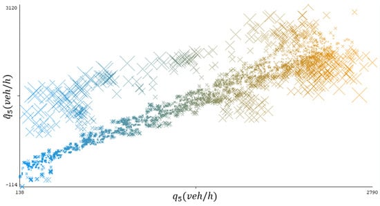
Figure 4.
Relationship between and .
Time-domain simulations of the examination are shown in Figure 5. Two scenarios are illustrated, i.e., an average traffic flow veh/h and a rush traffic flow veh/h with a congestion at the beginning of the simulation. Figure 5 illustrates that the generated prediction model is able to accurately approximate in both scenarios.
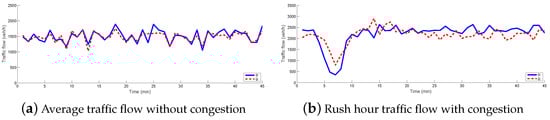
Figure 5.
Examples with the results of the data-driven analysis.
The examples show that the proposed data-driven model can be effective with regard to making a traffic flow prediction. The results of the prediction are satisfied under normal and congested traffic circumstances. However, the resulted prediction model (14) cannot be used for control purposes alone, because it is based on a linear formula, which is effective for short-term prediction. For long-term prediction, the nonlinear characteristics of the traffic flow must be taken into consideration, which is achieved by the interconnection of the data-driven prediction and the conventional traffic modeling approaches.
3. Formulating Control-Oriented Traffic Flow Prediction Model
In this section, the control-oriented model for traffic flow dynamics, in which the data-driven prediction model and traffic modeling principles are used together, is proposed.
In the formulation of traffic dynamics, the traffic network is gridded into N number of segments. The traffic flow of each segment is represented by a dynamical equation, which is based on the law of conservation. The relationship contains the sum of inflows and outflows for a given segment i. Traffic density (veh/km) is expressed as
where k is the index of the discrete time step; T is the discrete sample time; is the length of the segment; (veh/h) and (veh/h) are the inflow of the traffic in segments i and , and finally, (veh/h) is the sum of the controlled ramp inflow.
Another important relation of the traffic dynamics is the fundamental relationship which creates a connection between outflow , traffic density and average traffic speed []. The fundamental relationship is formed as
Conventionally, the fundamental relationship is derived through historic measurements and depends on several factors, as can be seen in, e.g., [,]. and are formed in the traffic flow model as nonlinear functions of traffic density [], such as and , where are nonlinear functions. In the modeling of the traffic flow dynamics, the impact of on can be considered in the nonlinear function of , such as
Function can be effectively formulated through polynomial relationships []. An example of , which depends on the and the presence of automated vehicles in the traffic, is illustrated in Figure 6.
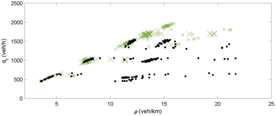
Figure 6.
Illustration of the relationship between (green: without automated vehicles; black: with automated vehicles).
The dynamics of the traffic flow based on (15) and (17) is written as
which contains the nonlinear characteristics of the fundamental diagram . The advantage of the expression (18) is that it incorporates the nonlinear behavior of the traffic flow dynamics, and thus, (18) can be effective for the long-term prediction of through . However, is derived based on historic measurements, which means that it has an increased error in terms of short-term prediction. Consequently, (18) uses only a small number of actual data.
The following model combines the data-driven prediction model and the conventional traffic model. The purpose of this solution is to eliminate the drawbacks of each method in the prediction. The highway in the case of the conventional traffic model is formed as a queue with one segment , while in the case of the data-driven model, the highway is divided into N number of sections. The prediction of the outflow of the highway is as follows:
where is the prediction from the data-driven model and is the prediction from the traffic model. The following form is applied: , in which . Moreover, the forgetting factor , is introduced, which depends on the step of the prediction p. In the case of , has high value, while the increase in p leads to the reduction in . Through the modification of , a balance of the prediction can be achieved. In a short-term prediction, has priority, while in a long-term prediction, has priority.
The prediction of the outflow at is formed as
The factors are the following. is expressed in the following form:
and thus, is also used in the prediction. is expressed based on (14), such as
where results from (14) and for all k.
Through the proposed traffic model, the prediction of the traffic flow can be updated through the results of the data-driven analysis. Through the increase in the value p, the impact of the data-driven model through is reduced; consequently, the emphasis of the nonlinear characteristics of the traffic flow is considered.
4. Optimal Control Design for Traffic Flow Maximization
The design of an optimal control was based on the previously formed enhanced traffic flow model. The purpose of the control design is to guarantee the maximum outflow of the traffic network through the inflow of the controlled ramp . Since the system contains disturbances, their impact on must be reduced. This leads to an optimization task.
In the control design of the traffic system, the following performance requirements must be guaranteed.
- It is necessary to achieve the maximum outflow of the traffic network , such as:where represents the length of the horizon. This performance specification is advantageous compared to the classical solution, which is based on the setting of related to critical density , as can be seen in, e.g., []. Namely, the setting of requires preliminary knowledge on the critical density of the traffic flow. Nevertheless, it depends on several factors, as can be seen in []. At the same time, in the proposed control strategy, data are obtained from the traffic system through data-driven analysis. This means that the result of the optimization can be effective without a fixed fundamental diagram.
- In the control task, the control inputs must be as small as possible. The control input , is a positive variable, which has physical limits. Moreover, it is necessary to limit its variation to prevent the rapid change during the actuation. Therefore, two constraints on are defined, such aswhere is the maximum of and is its maximum variation.
The traffic system has also disturbances within the inflow data, because the number of future entering vehicles is unknown, even if the routes of the automated vehicles are assumed to be known. Due to the ratio of automated vehicles, can be divided into known () and unknown () disturbances in the following way:
The known disturbances can be incorporated in the traffic flow maximization procedure as constant values. Thus, only a part of the disturbances, i.e., the unknown disturbances, can be handled in a worst-case scenario.
The form of the control task requires three components. First, the performance in (23) was used as an objective of optimization. Second, the performance (24) is handled as a constraint in the control design. Third, disturbance in (25) must be minimized in . Thus, the control design leads to a min–max task:
with the following constraints:
where are the bounds of the unknown disturbance. The results of the optimization are the intervention signals and the values of the unknown disturbances . The control signal at time step k is .
The solution of task (26) requires the joint handling of the minimization and maximization tasks. In practice, these are separated and an iterative solution is applied.
- First, the minimization task is solved for initial fixed values . The solution is achieved by an optimization algorithm, which is able to handle nonlinear constraints, as can be seen in, e.g., []. This results in values, which are used as fixed values during the solution of the maximization task in (26).
- Second, the maximization task is also solved by using values. The maximization task also results in values.
- The iteration procedure is stopped, when the relative errors of the solutions , in the actual and the previous steps are smaller than a predefined value.
5. Simulation Examples
In this section, the effectiveness of the proposed method is illustrated through simulation examples. In the examples, a 5 km-long highway section with three lanes for was selected illustration purposes. In the example, was set, meaning that the traffic flow contains a significant number of automated vehicles. Several simulations were performed in the VISSIM traffic simulator in order to determine the function . The illustration of a selected scenario is shown in Figure 7a. Figure 7a shows the variation of traffic flow volume, depending on highway section (axis X) and on time (axis Y). Here, the values of the volume in several small sections of the highway depending on the time are shown. There is a congestion at the end of the highway section at 10 min, which has a significant impact on the entire highway section. The reduced traffic flow has reached the 1 km section point at 20 min. The example shows that the dynamics of the traffic flow is close to the experience in the context of highway scenarios. In the illustration, the simulated data are synchronized, which is guaranteed by the data acquisition process in VISSIM. Figure 7b shows the derived fundamental diagram of the highway. The data for the determination of were obtained by various VISSIM simulations. The volume–density pairs of all simulation scenarios on this figure were matched through their time stamp in VISSIM. was approximated to a sixth-order polynomial form.
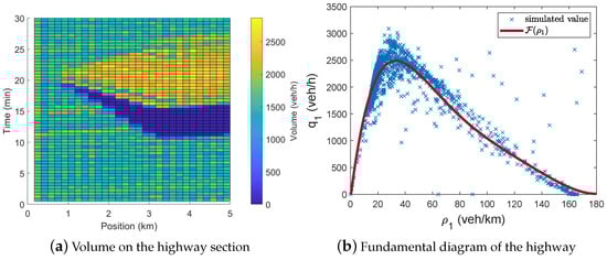
Figure 7.
Simulation example of the selected highway section.
The effectiveness of the outflow prediction is illustrated in Figure 8. The example presents the effectiveness of the integration of the data-driven and the classical traffic models for the prediction of the forthcoming traffic flow. Figure 8 shows the real outflow, which is approximated in three ways. First, illustrates the prediction made by the classical traffic model (18). In the simulation, the model uses as new data and as its state in all time step k. Although the model predicts the forthcoming congestion for high p values, it has a higher prediction error at low p values. Second, the data-driven prediction is shown by . The prediction model (14) uses as new data for all k step and states in the computation of . This model is unable to predict non-linearities due to its linear form. Consequently, predicts the real outflow for small p values, while for increased p values, significantly differs from the real-traffic flow. Third, the results of the interconnected model are shown in Figure 8. In the interconnection between and , the function is selected as if , otherwise . The selection guarantees the smooth transition between the interconnected signals. The predicted outflow approximates the real outflow on the entire term of the prediction.
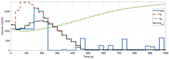
Figure 8.
Illustration of the outflow prediction.
The operation of the controlled system is shown in Figure 9. In the example, the 5 km-long-highway section has an on-ramp at the highway segment 1 km. The inflow on the ramp r can be controlled by traffic light. The purpose of the control is to guarantee the maximum outflow at the end of the highway section through the actuation of r. The inflows represent a traffic scenario, in which there is a rush hour in the middle of the simulation. The inflow is shown in Figure 9a and the inflow demand on the on-ramp is shown in Figure 9b. The inflow is limited by the computed r, which results in the real inflow . In the simulation, the variation limit is set to veh/h. Another result of the min–max optimization task is , which is illustrated in Figure 9c. The limits of are veh/h and veh/h. The role of the computation of is to characterize the worst-case scenario. For example, between 250 s and 1000 s, the worst-case is , which facilitates reduced outflow through a congestion. Although overestimates the real value of the unknown , it guarantees the avoidance of the traffic jam. The achieved outflow of the highway is illustrated in Figure 9d. It can be seen that the performance of the control, i.e., the maximization of the outflow, is achieved.
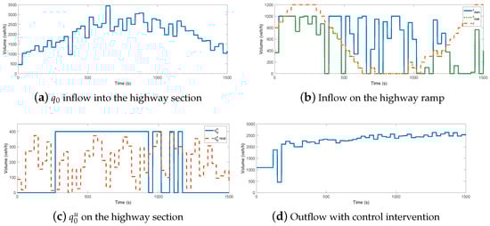
Figure 9.
Simulation on the controlled highway section.
Figure 10 presents two counter examples to illustrate the effectiveness of the proposed control strategy. Figure 10a illustrates the scenario without control, which means that the inflow enters the highway. Due to the increasing and , the traffic flow on the highway is over saturated, which leads to a congestion, between 900 s and 1500 s. The comparison of Figure 9d and Figure 10a shows the effectiveness of the traffic control system, i.e., the outflow is significantly higher due to the avoidance of congestion.
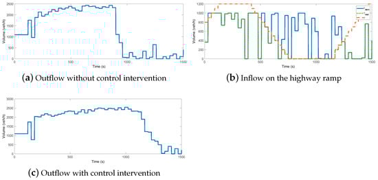
Figure 10.
Counter examples for the examination of the control.
The following simulation example is shown in Figure 10b,c. In this scenario, the control strategy is modified by the simplification of the optimization task (26), which leads to the following form:
such that
This means that the worst-case scenario is not considered during optimization. This results in increased inflow on the ramp, as can be seen in Figure 10b. In this scenario, the limitation of the inflow started at 450 s, while in the scenario of Figure 10b, r is reduced after 250 s. Although the achieved outflow is similar until 1000 s, its significant reduction in the simulation between 1000 s and 1500 s was due to the over saturation of the traffic flow.
6. Conclusions
This paper proposed an effective method for the prediction and maximization of traffic outflow on a highway. The results of the simulations showed that the prediction through the integration of data-driven and model-based methods can be improved compared to each prediction. Moreover, the examples on the control illustrated that maximum outflow during the entire traffic flow process can be achieved. Therefore, the proposed prediction and control design methods can be efficiently used as a theoretical control basis for highway traffic applications. Nevertheless, the proposed method requires a large number of data, from which the data-driven model is to be generated. Since the data-driven and model-based prediction blocks contain a large number of parameters, the implementation of the method for different types of highway sections (e.g., varying lane numbers and section lengths) can require the calculation of parameters.
The future challenge of the method is to improve the model-based prediction through learning-based features. Instead of using parameters in physical-based relationships, a possible way to achieve the traffic flow model is to tune the model parameters through the learning process. It requests enhanced learning features, with which the structure and the parameters of the model can be automatically selected, as can be seen in, e.g., []. Using this improvement, the advantages of the model-based prediction on an increased horizon can be exploited.
Author Contributions
Conceptualization, algorithms, B.N.; software D.F., Z.B.; methodology B.N.; supervision, P.G., B.N. All authors have read and agreed to the published version of the manuscript.
Funding
This research was supported by the Ministry of Innovation and Technology NRDI Office, within the framework of the Autonomous Systems National Laboratory Program. The research was partially supported by the Hungarian Government and cofinanced by the European Social Fund through the project “Talent management in autonomous vehicle control technologies” (EFOP-3.6.3-VEKOP-16-2017-00001). The work of Dániel Fényes was supported by the ÚNKP-21-3 New National Excellence Program of the Ministry for Innovation and Technology from the source of the National Research, Development and Innovation Fund.
Institutional Review Board Statement
Not applicable.
Informed Consent Statement
Not applicable.
Data Availability Statement
The data presented in this study are available on request from the corresponding author.
Conflicts of Interest
The authors declare no conflict of interest.
References
- Gáspar, P.; Németh, B. Predictive Cruise Control for Road Vehicles Using Road and Traffic Information; Springer: Berlin/Heidelberg, Germany, 2019. [Google Scholar]
- Frejo, J.R.D.; De Schutter, B. Logic-Based Traffic Flow Control for Ramp Metering and Variable Speed Limits—Part 1: Controller. IEEE Trans. Intell. Transp. Syst. 2021, 22, 2647–2657. [Google Scholar] [CrossRef]
- Frejo, J.R.D.; De Schutter, B. Logic-Based Traffic Flow Control for Ramp Metering and Variable Speed Limits—Part 2: Simulation and Comparison. IEEE Trans. Intell. Transp. Syst. 2021, 22, 2658–2668. [Google Scholar] [CrossRef]
- Liu, T.; Abouzeid, A.A.; Julius, A.A. Traffic Flow Control in Vehicular Multi-Hop Networks With Data Caching and Infrastructure Support. IEEE/ACM Trans. Netw. 2021, 28, 376–386. [Google Scholar] [CrossRef]
- Calvert, S.; Mahmassani, H.; Meier, J.-N.; Varaiya, P.; Hamdar, S.; Chen, D.; Li, X.; Talebpour, A.; Mattingly, S.P. Traffic flow of connected and automated vehicles: Challenges and opportunities. Road Veh. Autom. 2018, 4, 235–245. [Google Scholar]
- Kessels, F. Traffic Flow Modelling. In Introduction to Traffic Flow Theory through a Genealogy of Models; Springer: Berlin/Heidelberg, Germany, 2019. [Google Scholar]
- Schakel, W.; Van Arem, B.; Netten, B. Effects of cooperative adaptive cruise control on traffic flow stability. In Proceedings of the 13th International Conference on Intelligent Transportation, Funchal, Portugal, 19–22 September 2010; pp. 759–764. [Google Scholar]
- Talebpour, A.; Mahmassani, H.S. Influence of connected and autonomous vehicles on traffic flow stability and throughput. Transp. Res. Part C Emerg. Technol. 2016, 71, 143–163. [Google Scholar] [CrossRef]
- Calvert, S.C.; Schakel, W.J.; van Lint, J.W.C. Will automated vehicles negatively impact traffic flow? J. Adv. Transp. 2017, 1–17. [Google Scholar] [CrossRef]
- Liu, H.; Kan, X.D.; Shladover, S.E.; Lu, X.-Y.; Ferlis, R.E. Modeling impacts of cooperative adaptive cruise control on mixed traffic flow in multi-lane freeway facilities. Transp. Res. Part C Emerg. Technol. 2018, 95, 261–279. [Google Scholar] [CrossRef]
- Shi, X.; Li, X. Constructing a fundamental diagram for traffic flow with automated vehicles: Methodology and demonstration. Transp. Res. Part B Methodol. 2021, 150, 279–292. [Google Scholar] [CrossRef]
- Tajalli, M.; Mehrabipour, M.; Hajbabaie, A. Network-Level Coordinated Speed Optimization and Traffic Light Control for Connected and Automated Vehicles. IEEE Trans. Intell. Transp. Syst. 2021, 22, 6748–6759. [Google Scholar] [CrossRef]
- Wang, J.; Lu, L.; Peeta, S.; He, Z. Optimal toll design problems under mixed traffic flow of human-driven vehicles and connected and autonomous vehicles. Transp. Res. Part C Emerg. Technol. 2021, 125, 102952. [Google Scholar] [CrossRef]
- Sliwa, B.; Liebig, T.; Vranken, T.; Schreckenberg, M.; Wietfeld, C. System-of-systems modeling, analysis and optimization of hybrid vehicular traffic. In Proceedings of the 2019 IEEE International Systems Conference (SysCon), Orlando, FL, USA, 8–11 April 2019; pp. 1–8. [Google Scholar]
- Lv, Y.; Duan, Y.; Kang, W.; Li, Z.; Wang, F.Y. Traffic flow prediction with big data: A deep learning approach. IEEE Trans. Intell. Transp. Syst. 2015, 16, 865–873. [Google Scholar] [CrossRef]
- Li, L.; Yanwei, A.; Lin, Y.; Li, Z.; Li, Y. Robust causal dependence mining in big data network and its application to traffic flow predictions. Transp. Res. Part C 2015, 58, 292–307. [Google Scholar] [CrossRef]
- Dong, H.; Wu, M.; Ding, X.; Chu, L.; Jia, L.; Qin, Y.; Zhou, X. Traffic zone division based on big data from mobile phone base stations. Transp. Res. Part C 2015, 58, 278–291. [Google Scholar] [CrossRef]
- Bowman, C.N.; Miller, J.A. Modeling traffic flow using simulation and big data analytics. In Proceedings of the Winter Simulation Conference (WSC), Washington, DC, USA, 11–14 December 2016; pp. 1206–1217. [Google Scholar]
- Lu, H.; Sun, Z.; Yuan, W.; Qu, W. Big data-driven based real-time traffic flow state identification and prediction. Discret. Dyn. Nat. Soc. 2015, 2015, 1–11. [Google Scholar] [CrossRef] [Green Version]
- Kim, D.; Jeong, O. Cooperative Traffic Signal Control with Traffic Flow Prediction in Multi-Intersection. Sensors 2020, 20, 137. [Google Scholar] [CrossRef] [PubMed] [Green Version]
- Khan, S.; Nazir, S.; García-Magariño, I.; Hussain, A. Deep learning-based urban big data fusion in smart cities: Towards traffic monitoring and flow-preserving fusion. Comput. Electr. Eng. 2021, 89, 106906. [Google Scholar] [CrossRef]
- Liu, H.; Claudel, C.; Machemehl, R. Robust Traffic Control Using a First Order Macroscopic Traffic Flow Model. IEEE Trans. Intell. Transp. Syst. 2021. [Google Scholar] [CrossRef]
- Witten, I.H.; Frank, E. Data Mining Practical Machine Learning Tools and Techniques; Morgan Kaufmann Publishers: Burlington, MA, USA; Elsevier: Amsterdam, The Netherlands, 2005. [Google Scholar]
- Wang, Y.; Witten, I.H. Pace Regression. (Working Paper 99/12); University of Waikato, Department of Computer Science: Hamilton, New Zealand, 1999. [Google Scholar]
- Wang, Y.; Witten, I.H. Modeling for optimal probability prediction. In Proceedings of the Nineteenth International Conference in Machine Learning, Sydney, Australia, 8–12 July 2002; pp. 650–657. [Google Scholar]
- Ashton, W. The Theory of Traffic Flow; Spottiswoode, Ballantyne Co., Ltd.: London, UK, 1966. [Google Scholar]
- Messmer, A.; Papageorgiou, M. Metanet—A macroscopic simulation program for motorway networks. Traffic Eng. Control 1990, 31, 466–470. [Google Scholar]
- Treiber, M.; Kesting, A. Traffic Flow Dynamics: Data, Models and Simulation; Springer: Berlin/Heidelberg, Germany, 2013. [Google Scholar]
- Gartner, N.; Wagner, P. Analysis of traffic flow characteristics on signalized arterials. Transp. Res. Rec. 2008, 1883, 94–100. [Google Scholar] [CrossRef] [Green Version]
- Németh, B.; Bede, Z.; Gáspár, P. Control design of traffic flow using look-ahead vehicles to increase energy efficiency. In Proceedings of the 2017 American Control Conference (ACC), Seattle, WA, USA, 24–26 May 2015; pp. 3447–3452. [Google Scholar]
- Daganzo, C. Fundamentals of Transportation and Traffic Operations; Pergamon: Oxford, UK, 1997. [Google Scholar]
- Coleman, T.; Li, Y. An interior, trust region approach for nonlinear minimization subject to bounds. SIAM J. Optim. 1996, 6, 418–445. [Google Scholar] [CrossRef] [Green Version]
- Fényes, D.; Németh, B.; Gáspár, P. A Novel Data-Driven Modeling and Control Design Method for Autonomous Vehicles. Energies 2021, 14, 517. [Google Scholar] [CrossRef]
Publisher’s Note: MDPI stays neutral with regard to jurisdictional claims in published maps and institutional affiliations. |
© 2021 by the authors. Licensee MDPI, Basel, Switzerland. This article is an open access article distributed under the terms and conditions of the Creative Commons Attribution (CC BY) license (https://creativecommons.org/licenses/by/4.0/).