Abstract
In this paper, a new application of Bonobo (BO) metaheuristic optimizer is presented for PV parameter extraction. Its processes depict a reproductive approach and the social conduct of Bonobos. The BO algorithm is employed to extract the parameters of both the single diode and double diode model. The good performance of the BO is experimentally investigated on three commercial PV modules (STM6-40 and STP6-120/36) and an R.T.C. France silicon solar cell under various operating circumstances. The algorithm is easy to implement with less computational time. BO is extensively compared to other state of the art algorithms, manta ray foraging optimization (MRFO), artificial bee colony (ABO), particle swarm optimization (PSO), flower pollination algorithm (FPA), and supply-demand-based optimization (SDO) algorithms. Throughout the 50 runs, the BO algorithm has the best performance in terms of minimal simulation time for the R.T.C. France silicon, STM6-40/36 and STP6-120/36 modules. The fitness results obtained through root mean square (RMSE), standard deviation (SD), and consistency of solution demonstrate the robustness of BO.
1. Introduction
The concern over increasing energy costs, losses in the contemporary energy system and the greenhouse gas effect have shifted the world focus towards renewable energy resources [1]. Among the sources of renewable energy, solar energy (the PV system) is the fastest growing source of renewable energy in the world [2]. Unlike conventional power sources, the output power of the PV system depends on solar irradiation. Consequently, the increasing capacity of PV system installations poses a major challenge to power system operation and planning. Furthermore, PV system manufacturers only provide data relating to standard test conditions (STC), which are short circuit current, open circuit voltage, maximum power, current and voltage at maximum power point at irradiance, temperature and mass spectral distribution of 1000 W/m2, 25 °C and 1.5 air mass, respectively. However, this does not reflect the punitive environmental conditions in which PV systems are deployed for utilization [3]. As a result of this, the optimal extraction of PV model parameters is very important to analyze the dynamic characteristics of a PV module under different environmental conditions [4]. The accurate knowledge and characterization of PV modules are centred on the model parameters extracted, and this is important for several practical applications [5]. This will enhance the performance of the PV modules, fault analysis, quality control of the solar cells and, likewise, the maximum power point tracking [6]. Several models have been established to describe the input and output characteristics of the PV cells, the most popular is lumped parameter equivalent electrical circuit model: the single diode model (SDM) and the double diode model (DDM) [7]. However, the transcendental nature and existence of exponential terms in the model equations of the SDM and DDM make the optimum parameter extraction and efficient PV system simulation very challenging and complex by using basic functions [8,9,10]. In the light of these considerations, the challenges have attracted the attention of several researchers over the past years, and various computational procedures have been recommended.
Quite a number of methods are available for extracting parameters of both the SDM and DDM from the current-voltage (I–V) curves or datasheet [6,7,11]. The application of parameter extraction techniques that provide solutions based on empirical relations among several parameters or major points of PV characteristics is regarded as an analytical method [12]. Generally, analytical methods estimate PV cell parameters in one iteration. These methods are centred on deriving an observation and experimental relationship by solving a collection of equations that is obtained from the I–V (Current-Voltage) curve of the PV cell under the STC conditions [13,14]. The STC specifications can easily be obtained from the datasheet; these make analytical methods naturally handy. In spite of the benefits, analytical methods are prone to noise because of minimal selected points used in the calculation and PV degradation over time [15,16]. Furthermore, because of the non-linear model of the equations, and to ease computations, some assumptions are made which lead to inaccurate solutions [13,17]. Although these methods are befitting for the SDM, their aptness is yet to be substantiated for the DDM [3].
Conversely, numerical methods obtain the parameters by reducing the margin between simulated and experimental data points in multiple iterations. The numerical methods are known to be more dependable than the analytical methods [18]. Numerical methods can be divided into two categories: heuristic methods and deterministic methods. The latter relies on gradient information with initial constraint condition. As a result, they get stuck in a local search easily, which leads to erroneous and undependable solutions. In addition, the increment in decision parameters tends to reduce the accuracy of the optimizer [19,20]. Examples of these types of techniques are iterative curve-fitting [21], the Runge-Kutta method [22], Levenberg-Marquardt algorithm [23] and Newton-Raphson method [24]. To overcome the challenges associated with deterministic methods, several heuristic optimization approaches have been presented for the parameter extractions. Examples of these methods are genetic algorithms [25,26], particle swarm optimization [27], cuckoo search optimization [3], adaptive differential evolution algorithm [7], flower pollination algorithm [28], simulated annealing [20], harmony search [29], cat swarm optimization [30], coyote optimization algorithm [31], supply-demand-based optimization [32], improved chaotic whale optimization algorithm [10], firefly algorithm [33], differential evolution [34], symbiotic organisms search algorithm [35] and artificial bee colony [36]. Unlike deterministic methods, heuristic methods are notable for their global search operation and their efficacy towards handling non-linear functions without the requirements for gradient information. Furthermore, owing to their non-derivative nature, initial conditions are not required for the computation. Heuristic methods are robust, simple and easy to implement [31,32].
The performance and selection of any optimization methods are evaluated based on the speed of convergence, precision and ease of execution. Although the highlighted heuristic methods above have proved to be hopeful for parameter extraction, some heuristic algorithms contain control parameters, and the incorrect settings could lead to untimely and slow convergence [37,38]. Therefore, since accurate model parameters have not been established, any improvement in the fitting solution is highly indispensable for the model utilization. Moreover, considering the popular no free lunch theorem [39], no sole algorithm is appropriate to solve all optimization challenges. Therefore, the pursuit for different optimization algorithms that can effectively ascertain accurate parameters of PV cells is a cogent area of research. As a result, a Bonobo optimizer (BO) [40] for the parameter extraction of PV cells is presented in this study. The algorithm is selected because of its ease of implementation and fast computation time. Its process depicts a reproductive approach and the social conduct of Bonobos. The algorithm adopts the fission–fusion search approach of Bonobos, by splitting into smaller groups and later uniting for proficient optimization. The performance of the BO algorithm is extensively compared to MRFO [41,42], ABO [36], PSO [27], FPA [28] and SDO [32].
In terms of accuracy, convergence rate and dependability, experimental data reveals that BO outperforms the most recent well-established algorithms (e.g., MRFO, ABO, PSO, FPA and SDO). The following are the primary contributions of this paper:
- For the first time, a simple and time-saving metaheuristic algorithm called Bonobo optimizer (BO) has been presented to extract the electrical parameters of PV modules models based on several series of experiments.
- By combining different mating techniques found in bonobo culture, the suggested BO achieves a balance between exploration and exploitation.
- Throughout the search process, BO keeps the solution diverse, preventing premature convergence.
- BO avoids population stagnation by exploring diverse parts of a multidimensional search space while being guided by a group of bonobos with different mating strategies.
- The proposed BO is tested on different PV models datasets, and experimental results show that BO has better or competitive performance in comparison with other state of the art algorithms.
2. Mathematical Model of PV Module
A mathematical model can be employed to accurately depict the output characteristics of the PV model. This will portray the physical processes that occurs in the cell of the module. The most popular utilized model is the single diode and double diode PV cell model [17]. The parameter extraction of the PV cell is achieved by assuming the cells to be identical under similar operating circumstances. This criterion is used to devise the objective functions for the model description.
2.1. Single Diode Model (SDM)
Figure 1 shows the circuit model of a single diode PV cell. Using Kirchhoff’s Current Law (KCL), the output current, , of the model is calculated as [43]
where is the photocurrent, is the diode current and represents the shunt resistor current [32].
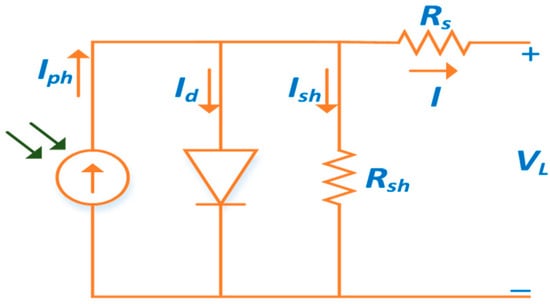
Figure 1.
Schematic diagram of SDM.
The Shockley’s diode equation, and the shunt resistor current can be represented as
where is the saturation current, is the diode ideal factor, is the output voltage, and are the shunt and series resistance, respectively, is the PV cell thermal voltage. denotes the Boltzmann constant, is the temperature of the junction in kelvin , is the electron charge.
By substituting Equations (2) and (3) into Equation (1), the output current of the PV cell module is represented as
It can be seen from Equation (4) that the single diode model has five parameters () that are required to be extracted.
2.2. Double Diode Model (DDM)
The ease of implementation and accuracy account for the utilization of the SDM. However, the DDM accounts for the effects of recombination current loss in the depletion region. This allows for a detailed model of the DDM and, therefore, advances the operation in some applications; specifically, in thin films at low irradiance [17,44]. Figure 2 depicts the model for the DDM with a second diode connected in parallel with the first. From KCL, the output current from is calculated as
where and are the first and second diode’s current, respectively. From Shockley’s diode equations, the two currents are represented as
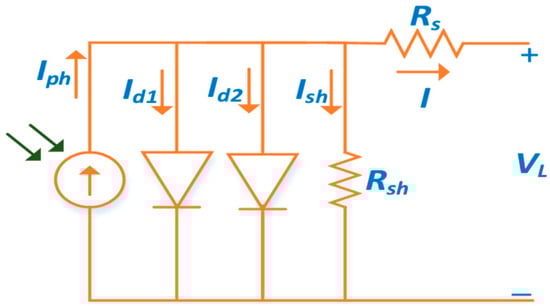
Figure 2.
Schematic diagram of DDM.
By incorporating Equations (6) and (3) in Equation (5), the output current of the DDM is represented as
where are the saturation currents. and are the diode ideality factors of the respective diodes. It is evident from Equation (7) that the DDM has seven unknown parameters ().
2.3. PV Module Model
By considering by solar cells with various connection in series and or parallel, the output current, , for the SDM and DDM can be represented as Equations (8) and (9), respectively
3. Bonobo Optimizer
Bonobo Optimizer (BO) is a new metaheuristic algorithm which is influenced by the reproductive approach and social conduct of Bonobos. It is a population-based algorithm developed by Amit Kumar Das et al. [40]. The algorithm adopts the fission-fusion search approach of Bonobos for proficient optimization. Bonobos partition into smaller groups, which are referred to as fission, for locating foods and later are reunited (fusion) at night for sleeping (refer to Figure 3). This distinct method was utilized in the algorithm to make the searching process more effective. Similarly to other heuristics, BO is also an algorithm based on population. An individual solution in the population is named a bonobo. The most dominant bonobo with the best rank hierarchy is called the alpha bonobo (αbonobo). Additionally, Bonobos advance through phase probability, which is either population diversity or selection pressure and through positive (PP) and negative (NP) phases, as shown in Figure 4. The counts of a successive number of iterations of PP and NP are called positive phase counts (ppc) and negative phase counts (npc), respectively. In order to reach the global optimum solution, the algorithm explores the natural behaviours and strategies of Bonobos. Bonobo utilizes four different mating strategies to create new Bonobos, they are: promiscuous, restrictive, consortship and extra-group mating [40].
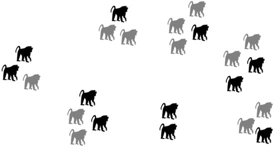
Figure 3.
Fission-fusion social groups of bonobos. Light figures are females; dark figures are males.
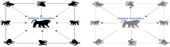
Figure 4.
Directions of movements of different bonobos with the higher probabilities. Dark figure is PP; Light figure is NP.
The mating strategies will change depending on the phase condition (positive (PP) or negative (NP)). The PP physically depicts the bonobo community when there is sufficient food, protection from neighboring communities, mating success and genetic variety among bonobos. The likelihood of the first two kinds of mating, i.e., promiscuous and restricted mating, will be greater during this period. Promiscuous mating makes an oestrus female available to both the alpha bonobo (i.e., the highest-ranking male in a group) and other lower-ranking males. However, in the event of restricted mating, only males of higher status may join. The NP, which denotes an unpleasant condition in the society, increases the likelihood of consortship mating and extra-group mating. A couple is isolated from their original community and spends their time together in a kind of mating called consortship. They rejoin their community after a few days or weeks. However, in the instance of extra-group mating, a female bonobo is observed mating with males from different communities. Additionally, the likelihood of extra-group mating is quite low in comparison to the possibility of mating with another group. These physical events are artificially reproduced in the suggested BO by the use of mathematics for optimization. The flowchart of the proposed algorithm is shown in Figure 5.
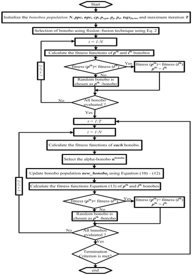
Figure 5.
Bonobo flowchart.
3.1. Promiscuous and Restrictive Mating Strategies
The phase probability parameter (pp) determines the mating approach of the Bonobo. At the initial stage, the value of pp is designated as 0.5, which is updated at every iteration. A new Bonobo is formed if a random number, r, generated as a value between 0 and 1, is found to be either less than or equal to pp as described in the following equation
where b is bonobo, and are the variables of the new offspring and αbonobo, respectively. as a value that varies between 1 and d number of variables. represent variable values of and bonobos, respectively. represents a value within the range from 0 to 1. The and are sharing coefficients for αbonobo and bonobos, respectively. The parameter: exists between −1 and 1. Promiscuous mating occurs when the best solution of bonobo yields a better result than bonobos. In this situation, the flag is allotted 1. Alternatively, it is referred to as restrictive mating. In this regard, the and αbonobo are assigned −1.
3.2. Consortship and Extra-Group Mating Strategies
These kinds of matings occur if phase is lesser than the random number, . Furthermore, if is equivalent to or less than the probability of extra-group , this will lead to updating of the solution via extra-group mating.
The is initialized with 0.5 with a gradual updating base on the nature of the evolution. The optimizes the searching process for the most promising result. and represent the lower and upper boundaries of the jth-variable, respectively.
In other cases, where the value of is found to be greater than that of , a new offspring is created using the consortship mating strategy as follows
where are random numbers between 0 and 1.
4. Objective Function
The implementation of parameter extraction requires the defining of a suitable algorithm for the objective function. Considering the fact that the best collection of solutions should produce the nearest fit to measured data, therefore, the best solution is obtained by minimizing the difference between the measured data and the calculated data. The most popular method to minimize the difference between the measured and calculated data is the root mean square error [6,10,11,31].
where is the calculated current value, is the measured current value and is the number of measured data.
5. Results and Discussion
BO, MRFO, ABO, PSO, FPA and SDO are utilized in determining parameters of the SDM and DDM. The parameters of models are obtained using the objection function in Equation (10). A notable standard solar data cell, R.T.C. France solar cell at 33 °C, which is extensively reported in the literature is selected as the benchmark for comparing and testing the algorithms [45]. The performance of the algorithms is further evaluated from the practical I-V curve of the single diode model of STM6-40 with 36 series cells at 51 °C and the single diode model of STP6-120 with 36 series cells at 55 °C. These datasets are obtained from [6,46]. To achieve a rational comparison, the three algorithms are compared under the same parameters as shown in Table 1, 500 iterations, 100 population size through 50 independent runs. The search ranges are determined based on boundaries conditions reported in [6]. The simulations were implemented on an Intel Core i5-8250U CPU@1.80 GHz, 16 GB under Window 1064bit with MATLAB 2020b.

Table 1.
Parameter boundary conditions.
5.1. Results for R.T.C France Single Diode Model (SDM) and Double Diode Model (DDM)
Since the accurate parameters are yet to be established, a meaningful way of establishing extracted parameters is the comparison of their fitness function (FF). As described in Equation (10), RMSE is adopted to evaluate the fitness function. Out of the 50 runs, the run with the minimum fitness function for each algorithm is selected. Figure 6 shows the fitness function with respect to the number of runs for the R.T.C. France SDM and DDM solar cell at 33 °C. From Table 2, BO exhibits the lowest standard deviation, minimum FF, and lowest maximum FF for both the SDM and DDM model. It is evident from the results that BO achieved optimum parameter extraction with minimal oscillations as compared to MRFO, ABO, PSO, FPA and SDO.
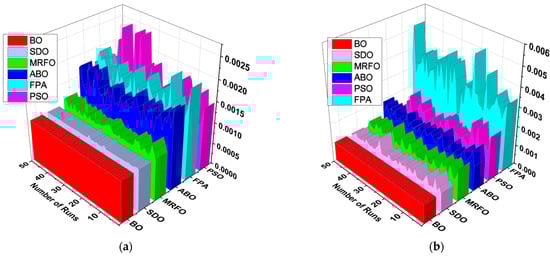
Figure 6.
Fitness Function R.T.C France solar cell; (a) SDM, (b) DDM.
Table 2.
Standard Deviation, Mean, FF minimum value, FF maximum value.
In order to substantiate values of the extracted parameters as shown in Table 3 and Table 4 the values are substituted in Equation (4) to obtain the I-V and P-V curve of Figure 7 and Figure 8 for both the SDM and DDM. The results demonstrate the ability of the BO algorithm to fit well with the experimental data. Table 5 and Table 6 show the experimental data and the calculated data for the I-V curve. Furthermore, BO utilized the lowest time in extracting the parameters for both the SDM and DDM, as shown in Figure 9, throughout the 50 runs.
Table 3.
R.T.C France SSD optimal extracted parameters for BO, MRFO, SDO, ABO, PSO and FPA.
Table 4.
R.T.C France DDM optimal extracted parameters for BO, MRFO, SDO, ABO, PSO and FPA.
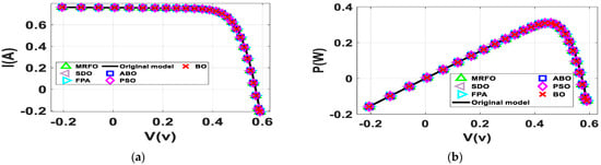
Figure 7.
R.T.C France SDM I-V (a) and P-V (b) curve.
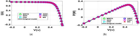
Figure 8.
R.T.C France DDM I-V (a) and P-V (b) curve.
Table 5.
R.TC France SSD experimental and calculated for BO, SDO, MRFO, ABO, PSO and FPA.
Table 6.
R.TC France DDM experimental and calculated for BO, SDO, MRFO, ABO, PSO and FPA.
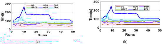
Figure 9.
Simulation time of RTC solar cell; (a) SDM, (b) DDM.
5.2. Results for STM6-40/36 and STP6-120/36
Table 7 and Table 8 provide information of the calculated standard deviation (SD), mean values and FF for both STM6-40/36 and STP6-120/36. From Figure 10, it is obvious that BO yields the smallest values of FF for both STM6-40/36 and STP6-120/36. STM6-40/36 for both MRFO and SDO show minimal SD and mean values but failed to achieve the smallest FF, as depicted in Table 7. Their smaller SD and mean are as a result of the close range of their FF, as shown in Figure 10. BO performs better than all the algorithms for STP6-120/36 in terms of SD, mean and FF. This demonstrates the heftiness of the BO algorithm for parameter extraction in comparison to other algorithms.
Table 7.
Standard Deviation, Mean, FF minimum value, FF maximum value for STM6-40/36.
Table 8.
Standard Deviation, Mean, FF minimum value, FF maximum value for STP6-120/36.
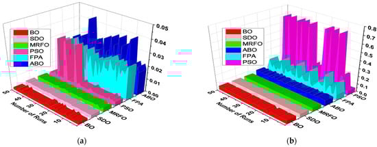
Figure 10.
Fitness function of single diode models; (a) STM6-40/36, (b) STP6-120/3.
The extracted results of the unknown parameters for both STM6-40/36 and STP6-120/36 are shown in Table 9 and Table 10, respectively. These results are selected from the runs that produce the minimum FF for each algorithm out of the 50 independent runs. These values are substituted in Equation (4) to obtain the calculated current value as shown in Table 11 and Table 12. The obtained results in Table 9 and Table 10 were further utilized to compare the fitness of the I-V and P-V curve of STM6-40/36 and STP6-120/36 with the experimental data, as described in Figure 11 and Figure 12. From the figures, it is evident that the calculated parameter by BO fits well with the experimental parameters. Figure 13 shows the simulation time for the 50 runs. The figures clearly reveal that the BO algorithm has the best performance in terms of the minimal simulation time for STM6-40/36 but not for STP6-120/36 throughout the 50 runs. FPA achieved the smallest simulation time for STP6-120/36 but without achieving the minimal FF. This is an indication of premature convergence by the FPA algorithm.
Table 9.
STM6-40/36 optimal extracted parameters for BO, MRFO, SDO, ABO, PSO and FPA.
Table 10.
STP6-120/36 optimal extracted parameters for BO, MRFO, SDO, ABO, PSO and FPA.
Table 11.
STM6-40/36 experimental and calculated results for BO, MRFO, SDO, ABO, PSO and FPA.
Table 12.
STP6-120/36 experimental and calculated results for BO, MRFO, SDO, ABO, PSO and FPA.
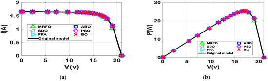
Figure 11.
STM6-40/36 I-V (a) and P-V (b) Curve.
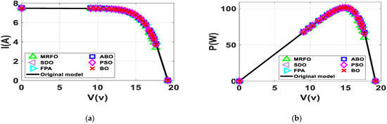
Figure 12.
STP6-120/36 I-V (a) and P-V (b) Curve.
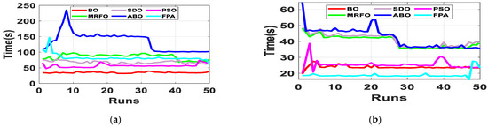
Figure 13.
Simulation time (a) STM6-40/36, (b) STP6-120/36.
5.3. Accuracy and Consistency of the Algorithms
In the same way as other types of metaheuristics algorithm, BO involves a stochastic model in its computational analysis. As a result, each run of the algorithm will not yield the same result. This creates an enormous challenge to determine the quality of the solution. Hence, it is imperative to investigate the consistency of the solution. By running the algorithms for 50 runs, a unique distinct pattern is obtained for the algorithms, which implies the parameters always unite at a resolute location, as shown in Figure 14, Figure 15, Figure 16, Figure 17, Figure 18 and Figure 19. The standard deviation of the BO algorithm computed denotes a good level of consistency, as shown in Table 13 and Table 14, for both the R.T.C France SDM and DDM.
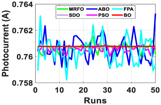
Figure 14.
R.T.C France SDM Photocurrent.
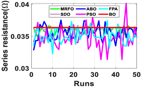
Figure 15.
R.T.C France SDM Series Resistance.
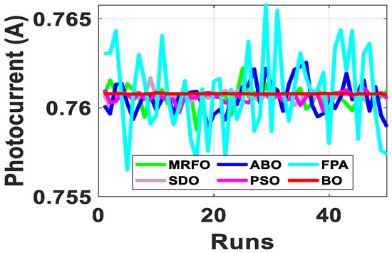
Figure 16.
R.T.C France SDM Photocurrent.
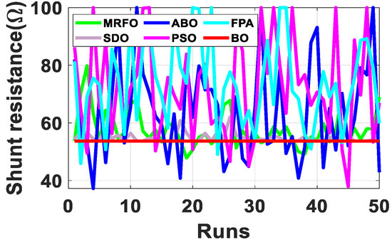
Figure 17.
R.T.C France DDM Shunt Resistance.
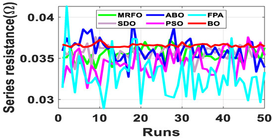
Figure 18.
R.T.C France DDM Series Resistance.
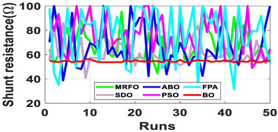
Figure 19.
R.T.C France Shunt Resistance.
Table 13.
R.T.C France SDM Standard Deviation.
Table 14.
R.T.C France DDM Standard Deviation.
Figure 20, Figure 21, Figure 22, Figure 23, Figure 24 and Figure 25 show the consistency patterns of the six algorithms for both STM6-40/36 and STP6-120/361. From the figures, it can be seen that BO achieves the highest level of consistency compared to other algorithms. The high deviation of BO as described in Table 15 and Table 16 is as a result of the high level of differences between its consistent level and deviation point.
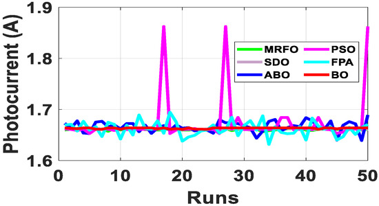
Figure 20.
STM6-40/36 Photocurrent.
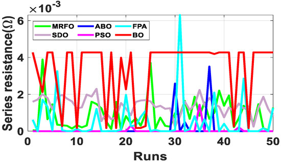
Figure 21.
STM6-40/36 Series Resistance.
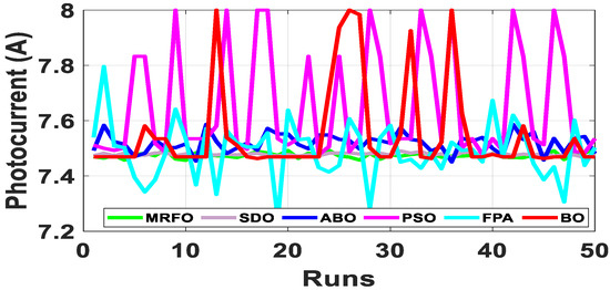
Figure 22.
STM6-40/36 Photocurrent.
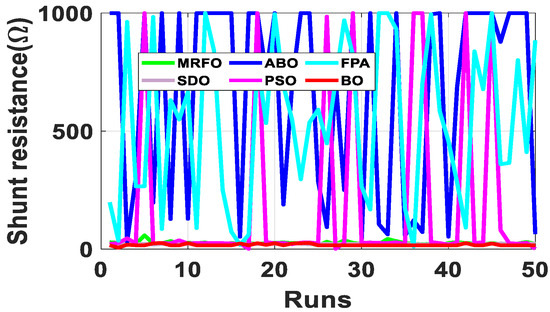
Figure 23.
STP6-120/361 Shunt Resistance.
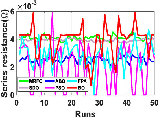
Figure 24.
STP6-120/361 Series Resistance.
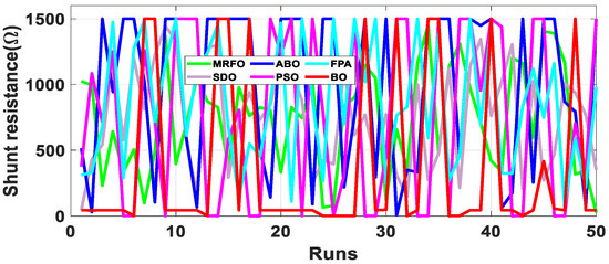
Figure 25.
STP6-120/361 Shunt Resistance.
Table 15.
Standard Deviation for STM6-40/36 parameters.
Table 16.
Standard Deviation for STP6-120/361 parameters.
6. Conclusions
This paper presents the new application of the BO algorithm for PV parameter extraction. The performance of the algorithm is compared with MRFO, ABO, PSO, FPA and SDO which are reported in the literature for PV parameter extraction. It is evident from the results that BO achieved the best precision. With respect to the fitness function, the BO achieved the lowest fitness function using the RMSE. The shortest time of the BO algorithm in extracting the parameters of the PV system also demonstrates its robustness and efficacy. Furthermore, the consistency of the BO algorithm also strengthened its resolve for PV parameter extraction compared with the five other algorithms. While the BO optimizer discussed in this paper has been shown to be rather effective, it may not be as effective in multi-objective issues. Other objectives that impact the on performance of PV systems should be included in future research. It would also be interesting to use BO to address other optimization problems, such as optimal sizing and siting of distributed generation, optimal load flow and optimal load dispatch.
Author Contributions
Conceptualization, A.A.A.-S.; Data curation, H.O.O.; Formal analysis, A.A.A.-S., H.M.H.F. and A.A.; Funding acquisition, F.A.A.; Investigation, H.O.O., K.A. and A.M.N.; Methodology, A.A.A.-S., H.O.O., H.M.H.F. and A.M.N.; Project administration, A.A.; Resources, F.A.A., H.M.H.F. and K.A.; Software, A.A.A.-S. and H.O.O.; Supervision, A.A.A.-S. All authors have read and agreed to the published version of the manuscript.
Funding
This work was supported by the Researchers Supporting Project number (RSP-2021/252), King Saud University, Riyadh, Saudi Arabia.
Institutional Review Board Statement
Not applicable.
Informed Consent Statement
Not applicable.
Data Availability Statement
The data presented in this study are available on request from the corresponding author.
Conflicts of Interest
The authors declare no conflict of interest.
References
- Rehmani, M.H.G.; Reisslein, M.G.; Rachedi, A.; Erol-Kantarci, M.G.; Radenkovic, M. Integrating Renewable Energy Resources into the Smart Grid: Recent Developments in Information and Communication Technologies. IEEE Trans. Ind. Inform. 2018, 14, 2814–2825. [Google Scholar] [CrossRef]
- Alturki, F.A.; Farh, H.M.H.; Al-Shamma’A, A.A.; Alsharabi, K. Techno-Economic Optimization of Small-Scale Hybrid Energy Systems Using Manta Ray Foraging Optimizer. Electronics 2020, 9, 2045. [Google Scholar] [CrossRef]
- Gude, S.; Jana, K.C. Parameter extraction of photovoltaic cell using an improved cuckoo search optimization. Sol. Energy 2020, 204, 280–293. [Google Scholar] [CrossRef]
- Alturki, F.A.; Al-Shamma’A, A.A.; Farh, H.M.H. Simulations and dSPACE Real-Time Implementation of Photovoltaic Global Maximum Power Extraction under Partial Shading. Sustainability 2020, 12, 3652. [Google Scholar] [CrossRef]
- Humada, A.M.; Hojabri, M.; Mekhilef, S.; Hamada, H.M. Solar cell parameters extraction based on single and double-diode models: A review. Renew. Sustain. Energy Rev. 2016, 56, 494–509. [Google Scholar] [CrossRef] [Green Version]
- Gao, X.; Cui, Y.; Hu, J.; Xu, G.; Wang, Z.; Qu, J.; Wang, H. Parameter extraction of solar cell models using improved shuffled complex evolution algorithm. Energy Convers. Manag. 2018, 157, 460–479. [Google Scholar] [CrossRef]
- Biswas, P.P.; Suganthan, P.; Wu, G.; Amaratunga, G.A. Parameter estimation of solar cells using datasheet information with the application of an adaptive differential evolution algorithm. Renew. Energy 2019, 132, 425–438. [Google Scholar] [CrossRef]
- Ortiz-Conde, A.; Garcia-Sanchez, F.; Muci, J. New method to extract the model parameters of solar cells from the explicit analytic solutions of their illuminated I–V characteristics. Sol. Energy Mater. Sol. Cells 2006, 90, 352–361. [Google Scholar] [CrossRef]
- Zhang, C.; Zhang, J.; Hao, Y.; Lin, Z.; Zhu, C. A simple and efficient solar cell parameter extraction method from a single current-voltage curve. J. Appl. Phys. 2011, 110, 064504. [Google Scholar] [CrossRef] [Green Version]
- Oliva, D.; el Aziz, M.A.; Hassanien, A.E. Parameter estimation of photovoltaic cells using an improved chaotic whale optimization algorithm. Appl. Energy 2017, 200, 141–154. [Google Scholar] [CrossRef]
- Jordehi, A.R. Enhanced leader particle swarm optimisation (ELPSO): An efficient algorithm for parameter estimation of photovoltaic (PV) cells and modules. Sol. Energy 2018, 159, 78–87. [Google Scholar] [CrossRef]
- Wei, D.; Wei, M.; Cai, H.; Zhang, X.; Chen, L. Parameters extraction method of PV model based on key points of I–V curve. Energy Convers. Manag. 2020, 209, 112656. [Google Scholar] [CrossRef]
- Chin, V.J.; Salam, Z.; Ishaque, K. An Accurate and Fast Computational Algorithm for the Two-diode Model of PV Module Based on a Hybrid Method. IEEE Trans. Ind. Electron. 2017, 64, 6212–6222. [Google Scholar] [CrossRef]
- Ibrahim, H.K.; Anani, N. Evaluation of Analytical Methods for Parameter Extraction of PV modules. Energy Procedia 2017, 134, 69–78. [Google Scholar] [CrossRef]
- Ishaque, K.; Salam, Z.; Taheri, H.; Shamsudin, A. A critical evaluation of EA computational methods for Photovoltaic cell parameter extraction based on two diode model. Sol. Energy 2011, 85, 1768–1779. [Google Scholar] [CrossRef]
- Gomes, R.C.M.; Vitorino, M.; Correa, M.B.D.R.; Fernandes, D.A.; Wang, R. Shuffled Complex Evolution on Photovoltaic Parameter Extraction: A Comparative Analysis. IEEE Trans. Sustain. Energy 2017, 8, 805–815. [Google Scholar] [CrossRef]
- Chin, V.J.; Salam, Z.; Ishaque, K. Cell modelling and model parameters estimation techniques for photovoltaic simulator application: A review. Appl. Energy 2015, 154, 500–519. [Google Scholar] [CrossRef]
- Lin, P.; Cheng, S.; Yeh, W.; Chen, Z.; Wu, L. Parameters extraction of solar cell models using a modified simplified swarm optimization algorithm. Sol. Energy 2017, 144, 594–603. [Google Scholar] [CrossRef]
- Saha, P.; Kumar, S.; Nayak, S.K.; Sahu, H.S. Parameter estimation of double diode photo-voltaic module. In Proceedings of the 2015 1st Conference on Power, Dielectric and Energy Management at NERIST (ICPDEN), Arunāchal Pradesh, India, 10–11 January 2015; pp. 1–4. [Google Scholar] [CrossRef]
- El-Naggar, K.; AlRashidi, M.; AlHajri, M.; Al-Othman, A. Simulated Annealing algorithm for photovoltaic parameters identification. Sol. Energy 2012, 86, 266–274. [Google Scholar] [CrossRef]
- Chan, D.; Phang, J. Analytical methods for the extraction of solar-cell single- and double-diode model parameters from I–V characteristics. IEEE Trans. Electron Devices 1987, 34, 286–293. [Google Scholar] [CrossRef]
- Elbaset, A.A.; Ali, H.; Sattar, M.A.-E. Novel seven-parameter model for photovoltaic modules. Sol. Energy Mater. Sol. Cells 2014, 130, 442–455. [Google Scholar] [CrossRef]
- Gow, J.; Manning, C. Development of a photovoltaic array model for use in power-electronics simulation studies. IEE Proc. Electr. Power Appl. 1999, 146, 193–200. [Google Scholar] [CrossRef]
- Raj, S.; Sinha, A.K.; Panchal, A.K. Solar cell parameters estimation from illuminated I–V characteristic using linear slope equations and Newton-Raphson technique. J. Renew. Sustain. Energy 2013, 5, 33105. [Google Scholar] [CrossRef]
- Zagrouba, M.; Sellami, A.; Bouaïcha, M.; Ksouri, M. Identification of PV solar cells and modules parameters using the genetic algorithms: Application to maximum power extraction. Sol. Energy 2010, 84, 860–866. [Google Scholar] [CrossRef]
- Sellami, A.; Bouaïcha, M. Application of the Genetic Algorithms for Identifying the Electrical Parameters of PV Solar Generators. In Solar Cells—Silicon Wafer-Based Technologies; InTech Europe: Rijeka, Croatia, 2011. [Google Scholar]
- Soon, J.J.; Low, K.S. Photovoltaic Model Identification Using Particle Swarm Optimization with Inverse Barrier Constraint. IEEE Trans. Power Electron. 2012, 27, 3975–3983. [Google Scholar] [CrossRef]
- Kumar, P.J.; Pillai, D.; Natarajan, R.; Chinnaiyan, K.V. Flower Pollination Based Solar PV Parameter Extraction for Double Diode Model. In Intelligent Computing Techniques for Smart Energy Systems; Springer: Singapore, 2020; pp. 303–312. [Google Scholar]
- Askarzadeh, A.; Rezazadeh, A. Parameter identification for solar cell models using harmony search-based algorithms. Sol. Energy 2012, 86, 3241–3249. [Google Scholar] [CrossRef]
- Guo, L.; Meng, Z.; Sun, Y.; Wang, L. Parameter identification and sensitivity analysis of solar cell models with cat swarm optimization algorithm. Energy Convers. Manag. 2016, 108, 520–528. [Google Scholar] [CrossRef]
- Chin, V.J.; Salam, Z. Coyote optimization algorithm for the parameter extraction of photovoltaic cells. Sol. Energy 2019, 194, 656–670. [Google Scholar] [CrossRef]
- Xiong, G.; Zhang, J.; Shi, D.; Yuan, X. Application of Supply-Demand-Based Optimization for Parameter Extraction of Solar Photovoltaic Models. Complexity 2019, 2019, 3923691. [Google Scholar] [CrossRef] [Green Version]
- Louzazni, M.; Craciunescu, A.; Aroudam, E.H.; Dumitrache, A. Identification of Solar Cell Parameters with Firefly Algorithm. In Proceedings of the 2015 Second International Conference on Mathematics and Computers in Sciences and in Industry (MCSI), Athens, Greece, 17 August 2015; pp. 7–12. [Google Scholar] [CrossRef]
- Chin, V.J.; Salam, Z. A New Three-point-based Approach for the Parameter Extraction of Photovoltaic Cells. Appl. Energy 2019, 237, 519–533. [Google Scholar] [CrossRef]
- Xiong, G.; Zhang, J.; Yuan, X.; Shi, D.; He, Y. Application of Symbiotic Organisms Search Algorithm for Parameter Extraction of Solar Cell Models. Appl. Sci. 2018, 8, 2155. [Google Scholar] [CrossRef] [Green Version]
- Oliva, D.; Cuevas, E.; Pajares, G. Parameter identification of solar cells using artificial bee colony optimization. Energy 2014, 72, 93–102. [Google Scholar] [CrossRef]
- Jiang, L.L.; Maskell, D.L.; Patra, J. Parameter estimation of solar cells and modules using an improved adaptive differential evolution algorithm. Appl. Energy 2013, 112, 185–193. [Google Scholar] [CrossRef]
- Eiben, A.; Hinterding, R.; Michalewicz, Z. Parameter control in evolutionary algorithms. IEEE Trans. Evol. Comput. 1999, 3, 124–141. [Google Scholar] [CrossRef] [Green Version]
- Wolpert, D.; Macready, W. No free lunch theorems for optimization. IEEE Trans. Evol. Comput. 1997, 1, 67–82. [Google Scholar] [CrossRef] [Green Version]
- Das, A.K.; Pratihar, D.K. A New Bonobo optimizer (BO) for Real-Parameter optimization. In Proceedings of the 2019 IEEE Region 10 Symposium (TENSYMP), Kolkata, India, 7–9 June 2019; pp. 108–113. [Google Scholar] [CrossRef]
- Alturki, F.A.; Omotoso, H.O.; Al-Shamma’A, A.A.; Farh, H.M.H.; Alsharabi, K. Novel Manta Rays Foraging Optimization Algorithm Based Optimal Control for Grid-Connected PV Energy System. IEEE Access 2020, 8, 187276–187290. [Google Scholar] [CrossRef]
- El-Hameed, M.A.; Elkholy, M.M.; El-Fergany, A.A. Three-diode model for characterization of industrial solar generating units using Manta-rays foraging optimizer: Analysis and validations. Energy Convers. Manag. 2020, 219, 113048. [Google Scholar] [CrossRef]
- Chin, V.J.; Salam, Z. Modifications to Accelerate the Iterative Algorithm for the Two-diode Model of PV Module. In Proceedings of the 2018 IEEE PES Asia-Pacific Power and Energy Engineering Conference (APPEEC), Sabah, Malaysia, 7–10 October 2018; pp. 200–205. [Google Scholar] [CrossRef]
- Chin, V.J.; Salam, Z.; Ishaque, K. An accurate modelling of the two-diode model of PV module using a hybrid solution based on differential evolution. Energy Convers. Manag. 2016, 124, 42–50. [Google Scholar] [CrossRef]
- Easwarakhanthan, T.; Bottin, J.; Bouhouch, I.; Boutrit, C. Nonlinear Minimization Algorithm for Determining the Solar Cell Parameters with Microcomputers. Int. J. Sol. Energy 1986, 4, 1–12. [Google Scholar] [CrossRef]
- Tong, N.T.; Pora, W. A parameter extraction technique exploiting intrinsic properties of solar cells. Appl. Energy 2016, 176, 104–115. [Google Scholar] [CrossRef] [Green Version]
Publisher’s Note: MDPI stays neutral with regard to jurisdictional claims in published maps and institutional affiliations. |
© 2021 by the authors. Licensee MDPI, Basel, Switzerland. This article is an open access article distributed under the terms and conditions of the Creative Commons Attribution (CC BY) license (https://creativecommons.org/licenses/by/4.0/).