Article

A Case Study of Thermal Evolution in the Vicinity of Geothermal Probes Following a Distributed TRT Method

1
Geo-Centre of Northern Bavaria, Chair of Geology, Friedrich-Alexander University Erlangen-Nuremberg, Schlossgarten 5, 91054 Erlangen, Germany
2
Institute of Information and Communication Technologies (ITACA), Universitat Politècnica de València, Camino de Vera S/N, 46022 València, Spain
*
Author to whom correspondence should be addressed.
Energies 2021, 14(9), 2632; https://doi.org/10.3390/en14092632
Submission received: 4 March 2021 / Revised: 29 April 2021 / Accepted: 30 April 2021 / Published: 4 May 2021
(This article belongs to the Special Issue Shallow Geothermal Energy 2021)

Abstract

:
To meet the stated climate change targets and to ensure the capability of meeting the current and future energy demands, there is an urgent need to develop renewable energy sources, such as geothermal systems. If geothermal systems are to be cost-efficient and are to enjoy public confidence, it is essential that they are designed and installed in accordance with the prevailing site-specific conditions. A thorough understanding of the thermal behaviour of the surrounding ground is, therefore, critical. In this work, we investigated temperature and its evolution in the vicinity of a shallow geothermal helix-shaped borehole heat exchanger (BHE). To measure the temperature close to the actual geothermal system, an additional U-tube probe was installed at the edge of the same borehole. A thermal load was then applied to the BHE, and the temperature was detected in the nearby U-tube. The temperature measurements were made with a GEOSniff monitoring device. To understand these localised temperature measurements in the context of the Valencia test site, ERT measurements were also performed. The GEOSniff device permits measurements to be made with very high depth resolution, which allows the thermal properties of the surrounding ground to be derived precisely, thus, enabling the identification of the different textural domains.

1. Introduction

Today, renewable energy suppliers must comply with national and international environmental targets, such as those published in the Paris Agreement of 2015. Shallow geothermal energy systems are an efficient means of satisfying space heating and cooling requirements, which represent a significant part of overall energy consumption. The environmental and economic potential for geothermal systems is, therefore, correspondingly large.
The installation and use of shallow geothermal systems requires preliminary estimation of the ground heat injection or extraction rates, which is often complicated due to the lack of homogeneity in the ground or the variation from the information provided by geological and soil maps to the actual conditions. To obtain reliable assessments of the thermal ground properties and the thermal parameters of the bedrock and to investigate the thermal behaviour of borehole heat exchangers (BHEs), thermal response tests (TRTs) are in widespread use [1,2].
In a standard TRT, the thermal response of the ground surrounding the borehole is recorded as a thermal front propagates through the surrounding ground [3]. As a result, different BHE systems that are installed in close proximity to each other can mutually interact and affect each other, which can produce negative thermal effects on both systems, which drastically reduces their efficiency [4].
The progression of the thermal front depends on the thermal properties of the soil, bedrock, and grouting material and can be characterised in terms of heat dissipation. These material-dependent thermal properties that produce variations regarding the discharge of temperature, can be described by the thermal diffusivity (α), which depends on the specific thermal conductivity (λ), thermal capacity (c), and density (ρ) of the ground.
α = λ/(ρ∙c).
Understanding these thermal interactions between and around the boreholes, which is the focus of the present study, is essential [5,6,7] for the proper assessment and sizing of planned fields in which several BHEs will be operating.
A standard TRT provides a single value for the average thermal efficiency of the borehole under test. However, this single value does not provide any insight into the effects of factors, such as a non-uniform ground profile or groundwater flow [8]. Systematic evaluations of different error sources are also rare [9] although some laboratory-scale investigations have been carried out [10,11].
To better understand the different thermal environments in and around boreholes, depth-resolved temperature measurements can be performed using advanced TRT methods [12]. These typically deploy fibre-optic cables for distributed temperature sensing (DTS) [3,13,14] with temperatures measured at distance intervals of approximately 100 cm [15]. TRT measurements should be carried out for a period of at least 72 h [11], as the initial phase of the measurement is dominated by thermal effects due to the grouting material and other transient factors [16,17].
Advanced TRTs are complex and expensive to perform and these additional costs might limit the degree to which these advanced techniques are used. Thus, although the depth-resolved temperature profile has significant potential for improving our interpretation of soil structure, advanced TRT measurements are still comparatively uncommon in the scientific literature [12]. To gain a better understanding of subsurface heat transfer (following the thermal heat injection of a TRT or the thermal stress of an operating geothermal borehole) and to acquire a clearer picture of the possible thermal interactions between adjacent BHEs, further research is urgently needed.
A range of software tools are currently available for dimensioning BHE fields [18,19,20,21]; however, their applicability depends on the quality of the underlying numerical model adopted. For instance, variations in the borehole thermal resistance may result in deviations between the field data and simulation results [22]. A complete understanding of the thermal properties within the BHE environment is, thus, crucial for meaningful interpretation of TRT measurements by proper assessment of the ground thermal properties and for the potential progression of more reliable software tools.
In this study, the rise in temperature close to the BHE was focused within a thermal test. To facilitate temperature monitoring of the ground in the immediate vicinity of the borehole, an additional single-U probe was inserted into the same borehole [23], similarly to the observer pipe applied by Aranzabal et al. [24] but within another distance to the system. This proceeding enabled a more ground-layer-dependent temperature measurement [24] than within the percolated helical BHE.
Temperature monitoring was carried out by a DTS system while a heat load was applied, similar to the approach used in [25]. In this work, however, the temperature was monitored with a GEOsniff device, which is a wireless spherical sensor that can be inserted into a geothermal probe, measures both the depth and temperature, and allows the temperature profile to be recorded with a vertical resolution (1–5 cm) much higher than is achievable in conventional DTS measurements using fibre-optic cables. With fibre-optic cables, a minimum distance of 50 cm between points for temperature sensing is needed, whereas the applied device records temperatures every 1–5 cm.
For investigations over distinctly greater depths or with another focus, a minor temperature measurement spatial resolution might be sufficient [26,27,28]. By using a wireless probe of this type, a distributed thermal response test (DTRT) can be performed. According to [12], no such DTRT has been published thus far. The applied thermal test follows this method of such a DTRT.
To obtain a more detailed picture of the structure of the surrounding ground, electrical resistivity tomography (ERT) measurements were also carried out over a 52-metre transect that passed over the borehole examined in this study. The results of the ERT measurements and stratigraphic information from the lithological column provide a useful means of validating the results from the DTRT investigation. In the field of geophysics, ERT is a non-invasive technique for determining the electrical resistivity of the ground. It is very sensitive with respect to those parameters that influence the electrical resistivity of the ground, such as the water content, water salinity, mineral composition, and material density [29,30,31,32,33,34].
In the past, ERT measurements have occasionally been used to investigate the thermal properties of the ground around shallow geothermal systems [6,35,36], sometimes in combination with DTS measurements. However, measuring temperature changes in ERT field tests can be challenging [37,38,39,40], particularly in unsaturated zones [16], unless the relative temperature differences are very high [40]. This statement is endorsed by this study. However, as the factors that influence ground electrical measurements also affect ground thermal properties, ERT data can be used to derive the thermal parameters [41,42]. As ERT measurements are particularly sensitive to the water content [31,43], the location of the groundwater level is easy to detect.
As stated, the main aim of this study was to obtain a better insight into the thermal coupling of vertical BHEs to the surrounding ground and the thermal evolution. For evaluation of this thermal evolution in different layers of the ground, a thermal test was performed with a thermal heat load of 1400 W during 24 h, which was applied on a helical BHE at a test site in Valencia. Therefore, on the one hand, the thermal behaviour should be analysed with high spatial resolution in the direct vicinity of the system, and, on the other hand, a broader view of the present ground should be introduced.
The results from the DTS investigation using GEOsniff measurements in the additional U-probe served for this high spatial resolution examination of the immediate surrounding of the BHE, whereas the ERT measurements enabled a more general picture of the ground at the Valencia test site and a rough characterisation of the actual thermal properties.

2. Materials and Methods
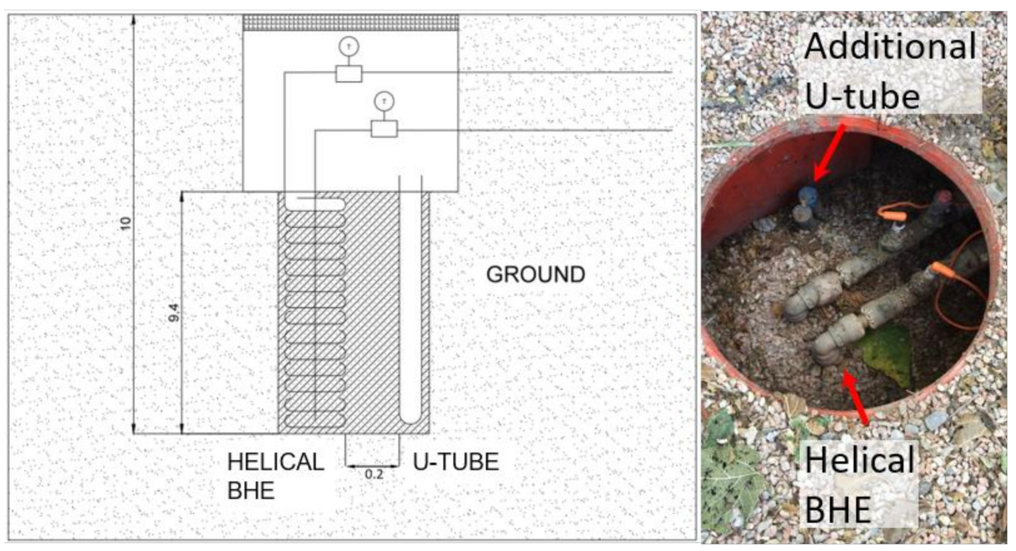
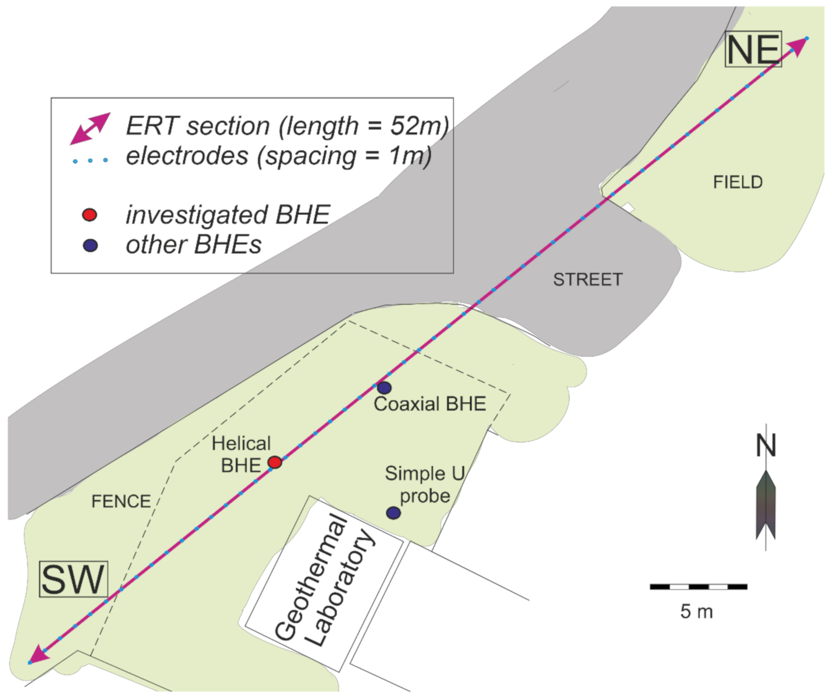
2.1. Test Site

The measurements were performed in May 2018 at the test site operated by the Geothermal Laboratory of the Universitat Politècnica de València (UPV). The site was built during the ‘Cheap GHSPs’ project and is currently in the course of becoming a European Centre of Excellence (ECoE).

2.1.1. European Centres of Excellence (ECoEs) for Shallow Geothermal Applications in Civil and Historical Buildings

“European centres of excellence for shallow geothermal application in civil and historical buildings” plans to build up a pan–European network in the framework of the European GEOCIVHIC project. based on past efforts, knowledge, and expertise with collaborating entities in different EU countries devoted to constantly teach and disseminate knowledge about shallow geothermal technology and scientific, technological, ICT, and managing innovations developed during the near past and future.
The aim is to help in knowledge dissemination and, in particular, to form future players/experts and to become an instrument to break down the barriers that shallow geothermal is still facing in transforming the geothermal energy as a standard source of H&C in building renovation, both civil and historical.
The research work described in this article is part of the activities to deepen the knowledge of the geological setting of the Geothermal Laboratory of the Universitat Politècnica de València (UPV) as part of its forthcoming role as European Centre of Excellence.

2.1.2. Test Site Description

Three different types of BHE (single-U, helix, and coaxial) were installed at the site with an appropriate monitoring and control system that enabled a stable level of thermal power to be injected between the inlet and outlet of the borehole [23]. This arrangement can be used to perform complex investigations with the objective of acquiring very detailed and accurate TRT measurements (as in this study) or to carry out thermal assessments of experimental boreholes.
The various BHE systems were around 10 m deep and were installed approximately 6.0-m apart. The effective borehole depth in the helix system used in this work was 9.4 m (Figure 1). The helix borehole was backfilled with a 4-0 mm silica sand (10% coarse sand and 90% fine gravel). When saturated, this grouting material has a thermal conductivity of 2.0–2.5 W/(m∙K). The pipe of the helical BHE had an external diameter of 25 mm with a pipe wall thickness of 2.3 mm. The diameter of the borehole was 450 mm, and the helical tube had an overall width of 360 mm. The axial pitch of the helical tube (i.e., the distance between adjacent turns on the helix) was 630 mm.
As the focus of this work was on determining the thermal properties of the surrounding ground layers, an additional single-U probe was installed within the same borehole at a distance of about 20 cm from the helix BHE. This U-tube had a diameter of 32 mm and was filled with water. The heat load was injected at the helical BHE, and the thermal behaviour was recorded at different depths within the single-U probe.

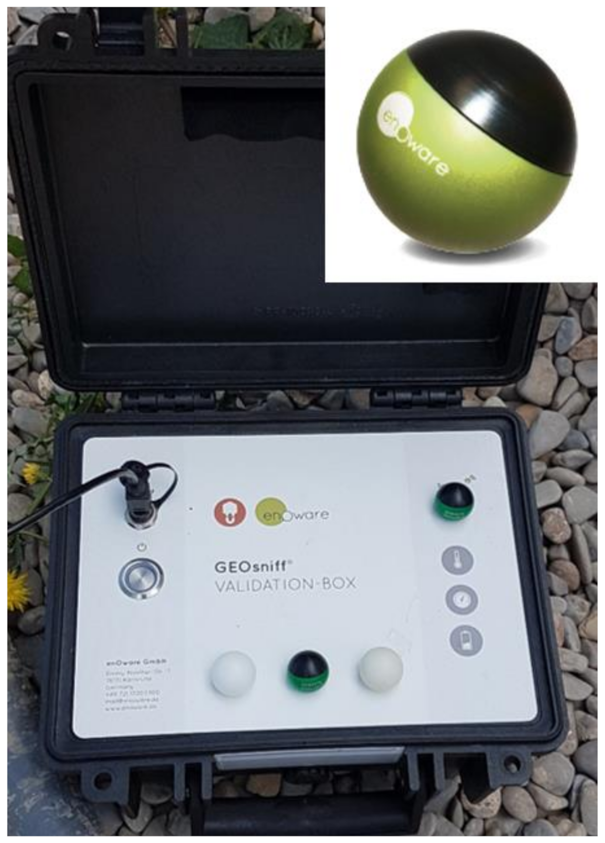
2.2. Temperature Monitoring

In contrast to other advanced TRT measurements, the temperature profile inside the single-U probe was determined with a GEOsniff device [12] manufactured by enoware. The measurements were carried out over a period of two days (16–17 May 2018). The green and black GEOsniff sensor ball (Figure 2) can be inserted into standard BHEs and measures temperature as a function of depth as it travels through the BHE tube. The spherical wireless sensor has a diameter of 20 mm.
The pressure sensor implemented in the GEOsniff device that records the hydrostatic pressure in the BHE has a stated absolute deviation of −60 to +20 mbar and a resolution of 1.0 mbar. The integrated temperature sensor has a measuring range from −10 to 35 °C, a deviation of 0.05 K and a resolution of <0.01 K. To classify these properties of the measurement device, a comparison between different devices was introduced by Aranzabal et al. [44].
The descent speed of the GEOsniff sensor ball is specified as about 6.5 m/min; however, this was not achieved in this study, as a special sensor casing from the manufacturer (GEOsniff CORD CLIP) was used to guide the GEOsniff ball down and out of the U-tube. As the descent speed was slower (around 1–2 m/min) due to the increased upward buoyant force but the measurement frequency of 1 Hz (1 measurement per second) was unchanged, the number of measurements per unit depth was significantly higher. Thus, this proceeding simply prolonged the measurement for a few minutes with the positive side effect of an increased spatial resolution (1–5 cm).
By placing the GEOsniff device in the tube and then retrieving it afterwards, the water column of the BHE tube was disturbed twice for each measurement. To obtain temperature measurements in an undisturbed medium that accurately reflected the temperature at a specific soil depth, the GEOsniff measurements were recorded only once an hour. After a measurement was made, which took about 15 min, the system was left undisturbed for a period long enough for the groundwater column to regain the temperature of the surrounding ground.

2.3. Geoelectrical Survey

To acquire greater insight into the ground in which the heat dissipation is occurring, an ERT measurement spanning two boreholes was also performed. This measurement was carried out on the second day of the temperature monitoring experiments, once while the heat load was still active (measurement ended at ~12:30) and once about 3–3.5 h later after shutting down the system (second measurement ended at ~16:00). For this investigation, a Lippmann ‘four point light’ resistivity meter (www.l-gm.de, accessed on 3 May 2021) was used.
The ERT transect was configured with 53 electrodes, each spaced 1.0 m apart. The measured section spanned two of the BHEs installed at the Valencia site (Figure 3), the investigated helical BHE at electrode 17 and the coaxial BHE at electrodes 24 + 25. The first six electrodes were positioned outside the property, where the transect crossed a channel system. After electrode 30, the line passed over the road behind the test site and ended in the roadside ditch at the edge of the field.
The multielectrode geoelectric tomography itself was carried out with the GeoTest software (www.geophysik-dr-rauen.de, accessed on 3 May 2021) using the Wenner array. Each determined electrical resistivity value was based on an average of a minimum of 10 and a maximum of 40 single measurements by using a stop criterion of 0.1% deviation between those measurements. The frequency of 4.16 Hz was used.
As a maximum current we set 50 mA, and, as a maximum voltage, we set 150 mV. Data inversion was performed with the Res2DInv software (https://www.geotomosoft.com/, accessed on 3 May 2021) using a refined model with a finer mesh and a robust inversion with a robust data constraint cutoff factor, which is less affected by noise but might produce a higher apparent resistivity RMS error. The complete Gauss Krüger calculation was used for inversion.

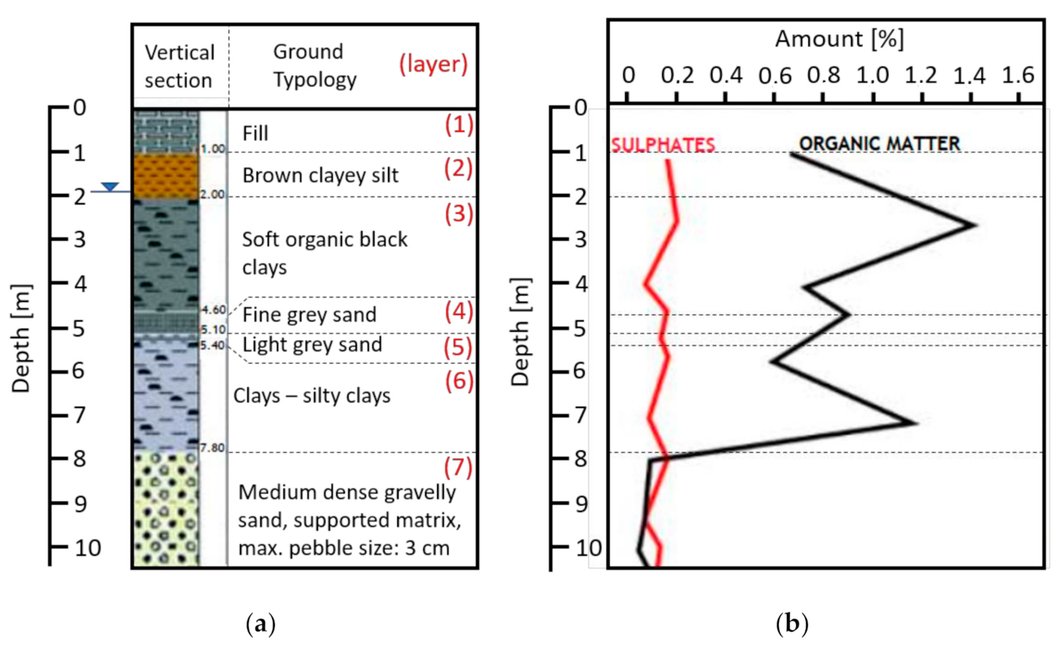
2.4. Lithological Column

The lithological properties (Figure 4) were characterised during the test site installation and drilling operations [23].
At the top of the column there is a one-metre-deep anthropogenic fill layer consisting of sandy soil material mixed with gravel. Below this fill layer is a transition zone with brown clayey silt down to a depth of 2 m. Below the transition zone are a series of argillaceous soil layers, uppermost of which is a black section with a significant amount of organic content down to a depth of 4.6 m.
The lower main section of the argillaceous domain comprises a light grey clay. The two main sections of the argillaceous domain are separated by fine sandy and loamy horizons each with a thickness of around 0.5 m. Below the argillaceous domain, we again find layers of coarse soil. This coarse zone starts with a layer of gravelly sand down to a depth of 10.6 m followed by a layer of gravel. At the time of geological analysis, the water table was detected at a depth of around 1.9 m.
A mineralogical analysis was also carried out (see Figure 4b), which indicated increased amounts of organic matter (0.8–1.4%) in the two main argillaceous domains.

2.5. Applied Heat Load

A constant thermal power load was applied to heat the helix system and to investigate the thermal properties of the soil in the vicinity of the helix BHE. The thermal injection power was 1400 W, and, since the helical borehole had a depth of about 10 m, the ratio was 140 W/m (Figure 5). This is not analogous to a conventional thermal power dissipation ratio of the helical borehole because this thermal power ratio produces very high temperatures in the heat exchanger (around 50 °C), which are not appropriate for use in a common geothermal heat pump.
The aim of this high thermal injection power is to achieve a high thermal load pulse in order to enable a more pronounced observation of its evolution in the different layers of the ground. The thermal power generated by the geothermal laboratory was injected into the borehole for about one day (Figure 5). The heat load was switched on at 12:30 and ran until 12:56 the next day. The inlet borehole temperature (T_in) varied from 40 to 52 °C while the thermal load was being applied. During this same period, the difference between T_in and the outlet temperature (T_out) remained fairly constant at around 8 degrees.
The sky was mostly clear on both the 16th and 17th of May 2018, with almost constant sunshine and an ambient temperature that occasionally exceeded 20 °C during the day (Figure 5). At night, the temperature dropped to around 10 °C. Figure 5 shows that the injection of thermal power remained essentially constant and the measured values of T_in and T_out were practically unaffected by any fluctuations in the ambient temperature.

3. Results

3.1. Electrical Resistivities

The results of the processed ERT data are shown in Figure 6. The maximum penetration depth achieved over the carried out ERT line according to the Res2DInv output was 8.5 m, which is a little less than the installation depth of the BHE. The errors after the fifth iteration were 3.1% and 2.9%, respectively.
Figure 6 provides clear evidence of horizontal layering. There was a distinct shift in the resistivity values at a depth of around 1.3 m. In the uppermost layer, the electrical resistivity was typically greater than 50 Ohm∙m, whereas, at depths greater than 1.3 m, the electrical resistivity of the ground was <20 Ohm∙m. Lower resistivity values in the near-surface section were only present close to the roadside ditch (20–40 Ohm∙m). By far, the highest resistivity values in the uppermost layer were found at locations close to the wells of both the helical BHE and the coaxial BHE (located at 23 m) and at the channel (at the fifth m of the section). These high resistivity zones correspond to air-filled cavities and/or loose packed material around the BHE wells.
This shift from higher to lower resistivities at a depth of 1.3 m represents the transition from sand and gravel within the first metre to the argillaceous layers below. ERT measurements are usually excellent at detecting the ground water table. However, in this case, the water table was only a few decimetres below this change in the soil grain size and thus the entire argillaceous domain should be nearly saturated due to capillary absorption. While this results in a sharp separation between the argillaceous domain and the coarse layer above, it also blurs the location of the deeper-lying water table.
In the second zone from 1.3 m down to about 8 m, the electrical resistivity was <20 Ohm∙m, which is typical of an argillaceous soil [45]. The electrical resistivity within this argillaceous domain gradually increased with depth, which indicates the presence of different argillaceous layers. The lower resistivity values in the upper part of this domain presumably reflect the presence of soft organic black clays, whereas the slightly higher resistivity values at the bottom part correspond to a silty clay layer. The deeper lying coarse layer of gravelly sand was not reached in the ERT measurement, or at least not to any relevant extent. In summary, the ERT data corresponded well with the layers identified in the lithologic column.
Considering the depicted fifth iteration of both measurements (Figure 6), there were some deviations of electrical resistivity values in the immediate environment of the helical BHE. Regarding the difference between these measurements during and after the heat load, the surface resistivity zone and the subsurface resistivity zone beneath 1.3 m, which is saturated, must also be treated separately. Within a depth of below 1.3 m, the difference was at a maximum of 2 Ohm∙m, which is not significant (Table 1).
Regarding the unsaturated zone only, directly at the helical BHE, after shutting down the heat load resistivity values occurred at about 30 Ohm∙m higher than with the heat load, and, at a distance of 1.5 m to the BHE, the differences were still 5–10 Ohm∙m. However, these differences cannot be related to only the switched off heat load because, within this time of around 3.5 h between both ERT measurements, the temperature in the direct vicinity of the BHE decreased by around 2 K (see Section 3.3).

3.2. Thermal Properties of the Investigated Area

After combining the information from the ERT measurements and from the lithologic column, we then assigned standard values for the thermal properties of each sub-layer that were taken from references [2] and [46] (Table 2).
The thermal conductivity values for saturated sandy soil of around 2.2–2.4 W/(m∙K) were very similar in both references [2] and [46]. However, for fine grained soil, the values quoted in [46] were distinctly lower. The soil-type classification used for unconsolidated materials in [2] is very general, comprising ‘sand’, ‘clay/silt’, ‘loam’, and ‘peat’. Nevertheless, the overall pattern showed that the two main argillaceous zones (the third and sixth layers in Table 2) exhibited the lowest thermal conductivities (even without considering the results of the organic content analysis in Figure 4b).

3.3. Temperature Variations in the Vicinity of the BHE

The GEOsniff measurements on 16 May 2018 were performed from 10:47 (‘undisturbed1’) to 18:44 (‘impact3’). On the second day, the measurements were carried out from 9:28 (‘impact4’) until 18:21 (‘down5’) (Figure 7). All measurements were performed inside the single-U probe installed at the edge of the borehole of the helical BHE, where the heat load was applied.
The first two measurements indicated an undisturbed soil temperature of around 21–22 °C (Figure 7). The temperature at the surface was around three degrees higher, which is likely due to the remarkably warm weather experienced at that time. Applying the heat load to the adjacent helix BHE system resulted in a general increase in temperature at all depths (‘impact1’ to ‘impact7’).
Arato et al. [16] stated that it takes about four hours for heat to pass through the BHE pipes and start to influence the ground. Luo et al. [17] suggested that the temperature development of heat carrier fluid in the first few hours was primarily influenced by the borehole grouting materials rather than the ground. As the temperature measurement probe is situated within the same borehole, these time specifications should also apply to the present study.
However, standard cement-based grouting was not used in this study but rather a silica sand with high thermal conductivity. The first clear increase in temperature was identified after a little more than 2 h (‘impact2’). The rate of heat dissipation was slightly greater than that stated in [16], and this may be due to the high thermal conductivity of the grouting used.
Closer inspection of the data from the ‘impact1’ measurement revealed a slight temperature increase at depths of 3.0–4.5 m and at 7.5–8.5 m. This may indicate the earlier onset of the temperature influence of the backfilling material, particularly in view of the fact that the next measurement (‘impact2’) showed a significant temperature rise of more than 2 °C at these depths. We, therefore, expect a significant thermal effect in the vicinity of the helical BHE system less than 2 h after the heat load application (i.e., between ‘impact1’ and ‘impact2’).
The ‘undisturbed2’ measurement was carried out while fluid circulation had already started. The slightly more jagged line in the upper 5 m of the temperature profile (Figure 7) might indicate heat dissipation of the thermal energy acquired by the feeder pipes between the geothermal laboratory and the BHE. However, the magnitude of this effect was not significant.
After about 23 h of thermal load injection, the overall temperature rose to 30–34 °C at depths below 1–2 m. This temperature increase in the vicinity of the helix system was around 10 degrees less than T_out and 18 degrees less than T_in. Figure 7 shows that, in the first 1.5 m below the surface, the temperature in this layer fell overnight (see ‘impact4’ and ‘impact5’) even though the heat load was still being applied. This temperature drop reflects the diurnal variation in ambient temperature, which is most strongly felt at the surface.
These diurnal changes induce variations in both the temperature and the moisture content of the soil. While the diurnal variation of soil moisture should be limited to the first few centimetres [47], temperature variations can be detected down to a depth of 2 m [48]. It seems that this effect can be detected in the layer above the groundwater-dominated domain. The groundwater level was located at around 1.9 m, directly above the argillaceous layers. As the capillary fringe extends a few decimetres above this groundwater level [30,49], the penetration depth of the diurnal effect described above of around 1.5 m appears to be limited to the unsaturated zone.
As the sky was almost entirely clear for the duration of the investigation, a relatively high diurnal variation in the surface air temperature was expected [50] and was confirmed by ambient temperature measurements (Figure 5). This high diurnal temperature range would also produce a more significant temperature variation in the near-surface soil compared with on cloudy days. In view of the impact of the diurnal temperature variation and interference from other factors affecting the thermal response, the near-surface layer down to a depth of 1.5 m is not considered further here.
We also do not discuss the water content as saturated conditions are assumed below a depth of 1.5–2.0 m. After all, seasonal changes of the ground temperature and moisture are not reflected in this study, which represents only a snapshot of time in mid-May. However, these considerations regarding the thermal properties of the ground are likely to be be pivotal mainly within the unsaturated zone. The temperature still will vary below the ground water level, which would cause another reached temperature level of the GEOsniff investigation.
As the temperature increase across the last four measurements (‘impact4’ to ‘impact7’) was relatively small, we assumed that the final temperatures reached represent a rough approximation of the maximum temperature achievable with the applied thermal load. Hence, this thermal test of 24 h is not in conformity with a precise TRT but with a shortened TRT [51].
Although a constant heat load was applied, the observed increase in temperature was depth-dependent. The temperature profile that developed had a characteristic shape (Figure 7) with two peaks, one around 3.5–4 m and one at a depth of 7.5–8 m. These peaks, which represent a localised relative temperature rise of approximately 1.5 degrees, were not present under the initial undisturbed conditions but were already evident in the ‘impact2’ measurement. The overall shape of the temperature profile remained unchanged on day two and was maintained for all measurements while the heat load was applied.
After switching off the heat load, the temperature gradient between the geothermal system and its vicinity began to subside and the heat dissipation gradually ceased. As the ground cooled, the thermal properties of the surrounding soil became less relevant and a smooth final temperature profile was recorded (see ‘down5’). It took about five hours for the temperature to fall by four degrees. Approximately three hours after the heat load was switched off, the temperature profile no longer exhibited the double-peak structure although the ground temperature was still significantly above the undisturbed temperature. Previous research [25] indicated that recovery measurements were barely affected by location.
Although the temperature effect is measured in homogenous backfill material, the temperature data reflects the thermal properties of the surrounding layers.

4. Discussion

The two temperature peaks observed, and the overall shape of the temperature profile reflect the different thermal properties of the surrounding ground layers. The shape of the temperature profile is unlikely to be due to the varying distance between the individual loops of the helical BHE and the single-U tube where the temperature measurements were made. If the shape of the helical BHE was responsible for the shape of the temperature profile, we would have expected to observe temperature peaks every 63 cm, which is the pitch of the helix.
However, only two peaks were observed around 400 cm apart. Moreover, the grouting material constitutes a uniform environment with homogeneous thermal properties below the water level. We, therefore, conclude that, as generally accepted, the temperature distribution within the geothermal system is based on the thermal properties of the surrounding ground.
Since ground material with a low thermal diffusivity will inhibit heat dissipation from the borehole, there will be relatively more heat accumulation in these areas. Consequently, at those depths where temperature peaks are measured, we expect the soil at that depth to exhibit lower thermal diffusivity or rather lower thermal conductivity values than the layers above and below it. It is evident from our data that the relatively high temperature values correlate to the two argillaceous domains, which indicates that these argillaceous zones generally have lower thermal conductivities than the coarser layers below and above them. This agrees with the tendency of the thermal properties derived from the VDI 4640 and [46] on the basis of the lithological column (Table 2).
The results of the ERT measurements generally confirm the lithological column. However, the ERT measurements also indicate a degree of variation within the argillaceous domain, although we observed a slight increase in the resistivity values with depth, which would not explain the two observed temperature peaks. To gain further insight into this issue, an analysis of the organic matter was carried out. It is generally accepted that organic matter in soil will reduce its thermal conductivity and, thus, its thermal diffusivity [52,53,54].
In our study, a small but non-negligible amount of organic matter was found within the argillaceous soil (Figure 4a). The low thermal diffusivity of the argillaceous domains is, therefore, due to a combination of the generally lower thermal conductivities of fine-grained soils and to the presence of a small amount of organic matter. It is of interest to note that the layers with the most organic content corresponded to those in which the temperature peaks were observed using the GEOsniff sensor. This suggests that even a minor amount of organic content has a significant influence on thermal properties and that this effect is superimposed due to the grain size distribution. Thus, such constitutional variations of the underground have to be considered for the precise dimensioning of BHE applications.
These outcomes with such a high spatial temperature resolution of this study were possible due to the GEOsniff application. Another study by Pambou et al. [28] that also used a submersible sensor provided a derivation of the ground thermal properties but with a larger scale (spatial resolution of 1 m). By applying more rough spatial resolutions, for example, by using a fibre-optic cable for DTS, every change of the ground constitutional variation might not be covered.
Acuna and Palm [26] used fibre-optic cables for temperature investigations while applying a TRT; however, they focused on the borehole thermal resistivity more than on the surrounding material. Hence, a high resolution was not decisive within their case. Aranzabal et al. [24,44] stated that novel instruments, such as the GEOsniff, have various advantages over standard sensors and fiber optics and also regarding the spatial resolution.
In research regarding TRT modelling, homogenous, isotropic, and temperature-independent materials representing the borehole are often assumed [25,27]. Due to the homogeneous granite underground in one case, within the verification measurements, no high resolution of temperature determination was needed, and the use of 10 m segmentations might be adequate [27].
Due to the slightly divergent aim of this study, which was to inject an unusual high amount of thermal energy per metre (140 W/m), compared with common TRTs, a clear increase of temperature could be achieved (partly around 10 degrees). This high amount of thermal energy per metre was possible due to the shallow depth of the investigated helical BHE system. In contrast, an application on deeper shallow geothermal systems (>100 m) may result in heat injection values between 5–30 W/m and a lesser temperature increase [26,27].
The results of Pambou et al. [28] did not exceed values of around 55 W/m and a temperature increase of 1–2 degrees by applying a relative high heat injection rate due to the system length. Although, a similar heat load was applied, for instance around 1500 W [24], the reached temperatures were distinctly lower than within this study (inlet temperature ≈ 50 °C) due to the system depth. Regarding a further investigation [55], where a similar power load was applied on a 15 m deep helical BHE, relative high temperatures (up to 45 °C) could have been reached. However, the temperature difference between the inlet and outlet temperature was only about 3 degrees, whereas this differential within our study was around 8 degrees, which is likely due to the difference in the ground thermal conditions. Mainly argillaceous layers (silt + silty clay) were stated there. Nevertheless, a distinctly higher amount of organic material might be present, as a 2.5 m thick peat layer was described [55].
While applying a heat load, the temperature development within such a short system as used within this study might be more uniform, whereas a deeper BHE produces an irregular temperature distribution over the depth [14,27]. Thus, the results of this study may be applied within subsequent analysis without an otherwise obligatory depth related correction.
Regarding the thermal evolution within the vicinity of the borehole (a 20 cm distance to the helical system) the measured temperatures were 18 degrees less than the inlet temperature and 10 degree less than the outlet temperature, which represents a far more significant temperature decrease within the same borehole as a 2-degree difference within the research of Aranzabal et al. [24]. This can be clarified by the different distance from the observer pipe to the geothermal system (20 cm vs. <5 cm) where the heat load was applied and by the much higher temperature gradient, which was achieved within this study.
Regarding the temperature development of the beginning recovery phase, this study confirms certain findings ascertained by numerical simulations: There, as set values, the referenced research [25] used a thermal conductivity of 1.2 W/(m∙K) for the grout and 2.5 W/(m∙K) for the surrounding material. With these settings, a general temperature loss 5 h after stopping the heat injection within the vicinity of the borehole of around 4 degrees was simulated, which fits very well with the measured temperature loss of this study (4–5 degrees after 5–6 h).
The generated data within this study can be used to build or refine numerical models in order to acquire greater insight into the details of heat distribution and heat dissipation in the vicinity of BHEs. Numerical simulation studies could also enable the effects of different heat transfer scenarios to be examined, such as the directional heat flow rather than only the lateral heat dissipation. To place these findings within a broader context, similar investigations using other soil configurations are needed. Field tests should also be carried out using different grouting materials, and the results should be analysed to classify their impact on heat dissipation as Borinaga-Treviño et al. [56] did.
The findings of this study might also be used to develop new or to refine existing simulation models for geothermal applications. There is the potential to use the measured temperature profiles to determine other parameters, such as the borehole thermal resistance [25,26,27]. Additionally, a Darcy flow analysis or a Péclet number analysis could be performed by interpreting the temperature logs [28]. The derivation of these hydraulic quantities may also support the idea of differentiating between areas in which heat is primarily transferred by conduction and those in which the convection dominates, as introduced in [14].
As demonstrated within this research, ERT measurements can significantly improve the insights regarding the hydraulic ground properties. As the ERT measurements showed clear horizontal layering without significant lateral inhomogeneity, the results of the temperature monitoring study should be applicable to all parts of the ERT transect, including the locations of the other BHE.

5. Conclusions

This case study demonstrated that DTS can be used to draw conclusions regarding the thermal properties of the ground surrounding a geothermal system. By combining the results of this thermal test following a DTRT, the ERT measurements, and additional analyses, two parameters that have a significant impact on the thermal behaviour of the ground were identified: the soil texture and the amount of organic matter.
The specific outcomes of this study are:
  • Diurnal temperature fluctuations were relevant in the near-surface coarse fill layer and, to some extent, in the subjacent transition zone down to the capillary fringe of the groundwater level. Short-term variations in the atmospheric temperature at the surface were found to influence the temperature profile down to a depth of around 1.5 m.
  • The main textural soil classes were distinguished by ERT, and the results showed that the recorded localised temperature profiles were transferable laterally to other parts of the ERT transect.
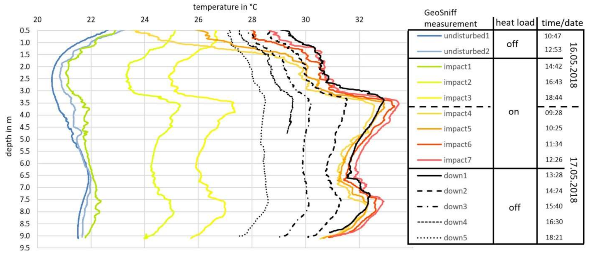
  • A significant thermal effect in the vicinity of the helical BHE was observed less than two hours after the heat load application. This early onset was attributable to the high thermal conductivity of the grouting used in this study.
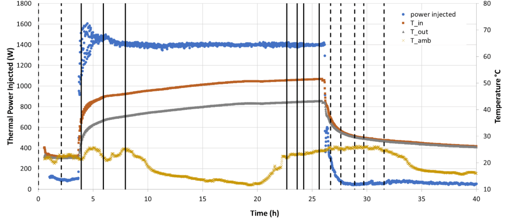
  • When a heat load with an inlet temperature of 40–50 °C was injected, the temperature in the vicinity (distance of about 20 cm) of the geothermal system was around 18 °C lower, while the difference between the inlet and outlet temperatures (T_in–T_out) was about 8 °C.
  • The high-resolution distributed temperature sensing technique used in this study produced a detailed temperature profile in which the two argillaceous layers of low thermal diffusivity were identified by the corresponding peaks in the temperature profile. The low thermal diffusivity values in these regions were explained by the generally lower thermal conductivities of the surrounding fine-grained soil materials. At any one time, the relative temperature difference within a single temperature profile was about 3–4 °C, which was related to the ground texture.
  • An increased fraction of organic matter in the argillaceous domains might also contribute to the lower thermal conductivity of these layers.
With these outcomes, a precise picture of the thermal behaviour for different ground layers within the investigated case is available. Due to seasonal temperature and moisture variations and ground-dependent thermal behaviour, a general transferability of the results to other BHEs cannot be stated. The thermal evolution particular within the saturated zone should be representative for similar ground conditions and should be considered for future helical BHE dimensioning, by applying similar thermal tests and TRTs.

Author Contributions

Conceptualization, H.S., B.B., and D.B.; Data curation, H.S.; Formal analysis, H.S.; Funding acquisition, J.U. and D.B.; Investigation, H.S., B.B., J.W., J.M.C., and D.B.; Methodology, H.S. and J.W.; Project administration, D.B.; Resources, J.U. and D.B.; Software, H.S.; Supervision, J.U. and D.B.; Validation, H.S., B.B., and J.M.C.; Visualization, H.S. and B.B.; Writing–original draft, H.S.; Writing–review and editing, H.S., B.B., J.W., and J.M.C. All authors have read and agreed to the published version of the manuscript.

Funding

This research work has been supported financially by the European Cheap-GSHPs Project (funded by the European Union’s Horizon 2020 research and innovation program under grant agreement No 657982) and by the European GEO4CIVHIC Project (funded by the European Union’s Horizon 2020 research and innovation program under grant agreement No 792355).

Data Availability Statement

The acquired data of this study can be provided by the authors.

Acknowledgments

This work has received funding from the European Union’s Horizon 2020 Research and Innovation program under grant agreement Nos. (657982) and (792355).

Conflicts of Interest

The authors declare no conflict of interest. The funders had no role in the design of the study; in the collection, analyses, or interpretation of data; in the writing of the manuscript, or in the decision to publish the results.

References

  1. Badenes, B.B.; Pla, M.; Ángel, M.; Lemus-Zúñiga, L.-G.; Mauleón, B.S.; Urchueguía, J.F. On the Influence of Operational and Control Parameters in Thermal Response Testing of Borehole Heat Exchangers. Energies 2017, 10, 1328. [Google Scholar] [CrossRef] [Green Version]
  2. VDI. Technical Rule 4640-1. Thermal Use of the Underground; Fundamentals, Approvals, Environmental Aspects; VDI, Beuth Publishing House: Berlin, Germany, 2010. [Google Scholar]
  3. Hakala, P.; Martinkauppi, A.; Martinkauppi, I.; Leppäharju, N.; Korhonen, K. Evaluation of the Distributed Thermal Response Test (DTRT): Nupurinkartano as a case study. In Report of Investigation 211; Geological Survey of Finland: Espoo, Finland, 2014; ISBN 978-952-217-306-5. [Google Scholar]
  4. Belliardi, M.; Soma, L.; Pasquali, R.; Sanner, B.; Zarrella, A.; De Carli, M.; Galgaro, A.; Perego, R.; Pera, S.; Badenes, B.; et al. Recommendations for the Planning and Implementation of New GSHP Systems in Dens Urban Environments and Related Tool. Deliverable D6.3. 2020; Available online: https://geo4civhic.eu/wp-content/uploads/2020/03/GEO4CIVHIC-D6.3.pdf (accessed on 3 May 2021).
  5. Mielke, P.; Bauer, D.; Homuth, S.; Götz, E.A.; Sass, I. Thermal effect of a borehole thermal energy store on the subsurface. Geotherm. Energy 2014, 2, 5. [Google Scholar] [CrossRef] [Green Version]
  6. Comina, C.; Giordano, N.; Ghidone, G.; Fischanger, F. Time-Lapse 3D Electric Tomography for Short-time Monitoring of an Experimental Heat Storage System. Geosciences 2019, 9, 167. [Google Scholar] [CrossRef] [Green Version]
  7. Gultekin, A.; Aydin, M.; Sisman, A. Effects of arrangement geometry and number of boreholes on thermal interaction coefficient of multi-borehole heat exchangers. Appl. Energy 2019, 237, 163–170. [Google Scholar] [CrossRef]
  8. Luo, J.; Rohn, J.; Xiang, W.; Bayer, M.; Priess, A.; Wilkmann, L.; Steger, H.; Zorn, R. Experimental investigation of a borehole field by enhanced geothermal response test and numerical analysis of performance of the borehole heat exchangers. Energy 2015, 84, 473–484. [Google Scholar] [CrossRef]
  9. Witte, H.J. Error analysis of thermal response tests. Appl. Energy 2013, 109, 302–311. [Google Scholar] [CrossRef]
  10. Firmbach, L.; Giordano, N.; Comina, C.; Mandrone, G.; Kolditz, O.; Vienken, T.; Dietrich, P. Experimental heat flow propa-gation within porous media using electrical resistivity tomography x (ERT). In Proceedings of the European Geothermal Con-gress, Pisa, Italy, 3–7 June 2013; pp. 3–7. [Google Scholar]
  11. Urchueguía, J.F.; Lemus-Zúñiga, L.G.; Oliver-Villanueva, J.V.; Badenes, B.; Mateo Pla, M.A.; Cuevas, J.M. How Reliable Are Standard Thermal Response Tests? An Assessment Based on Long-Term Thermal Response Tests Under Different Operational Conditions. Energies 2018, 11, 3347. [Google Scholar] [CrossRef] [Green Version]
  12. Wilke, S.; Menberg, K.; Steger, H.; Blum, P. Advanced thermal response tests: A review. Renew. Sustain. Energy Rev. 2020, 119, 109575. [Google Scholar] [CrossRef]
  13. Fujii, H.; Okubo, H.; Nishi, K.; Itoi, R.; Ohyama, K.; Shibata, K. An improved thermal response test for U-tube ground heat exchanger based on optical fiber thermometers. Geothermics 2009, 38, 399–406. [Google Scholar] [CrossRef]
  14. Lehr, C.; Sass, I. Thermo-optical parameter acquisition and characterization of geologic properties: A 400-m deep BHE in a karstic alpine marble aquifer. Environ. Earth Sci. 2014, 72, 1403–1419. [Google Scholar] [CrossRef]
  15. Kühl, J.U.; Lehr, C. Geothermische Messungen für die oberflächennahe Geothermie. In Handbuch Oberflächennahe Geothermie; Bauer, M., Freeden, W., Jacobi, H., Neu, T., Eds.; Springer Spektrum: Berlin, Germany, 2018; pp. 613–635. [Google Scholar] [CrossRef]
  16. Arato, A.; Boaga, J.; Comina, C.; De Seta, M.; Di Sipio, E.; Galgaro, A.; Giordano, N.; Mandrone, G. Geophysical monitoring for shallow geothermal applications—Two Italian case histories. First Break 2015, 33, 75–79. [Google Scholar] [CrossRef]
  17. Luo, J.; Rohn, J.; Xiang, W.; Bertermann, D.; Blum, P. A review of ground investigations for ground source heat pump (GSHP) systems. Energy Build. 2016, 117, 160–175. [Google Scholar] [CrossRef]
  18. Eskilson, P.; Claesson, J. Simulation model for thermally interacting heat extraction boreholes. Numer. Heat Transf. 1988, 13, 149–165. [Google Scholar] [CrossRef]
  19. Hellström, G.; Sanner, B. Software for dimensioning of deep boreholes for heat extraction. In Proceedings of the International Conference on Thermal Energy Storage (Proc. Calorstock), Espoo, Finland, 22–25 August 1994; pp. 195–202. [Google Scholar]
  20. Shonder, J.A.; Baxter, V.; Thornton, J.; Hughes, P. A new comparison of vertical ground heat exchanger design methods for residential applications. ASHRAE Tran. 1999, 105, 1179. [Google Scholar]
  21. Schulte, D.O.; Rühaak, W.; Welsch, B.; Sass, I. BASIMO—Borehole heat exchanger array simulation and optimization tool. Energy Procedia 2016, 97, 210–217. [Google Scholar] [CrossRef] [Green Version]
  22. Cullin, J.R.; Spitler, J.D.; Montagud, C.; Ruiz-Calvo, F.; Rees, S.J.; Naicker, S.S.; Konečný, P.; Southard, L.E. Validation of vertical ground heat exchanger design methodologies. Sci. Technol. Built Environ. 2015, 21, 137–149. [Google Scholar] [CrossRef]
  23. Pla, M.A.M.; Badenes, B.; Lemus, L.; Urchueguía, J.F. Assessing the Shallow Geothermal Laboratory at Universitat Politècnica de Valéncia. In Proceedings of the European Geothermal Congress, Den Haag, The Netherlands, 11–14 June 2019. [Google Scholar]
  24. Aranzabal, N.; Martos, J.; Stokuca, M.; Pallard, W.M.; Acuña, J.; Soret, J.; Blum, P. Novel instruments and methods to estimate depth-specific thermal properties in borehole heat exchangers. Geothermics 2020, 86, 101813. [Google Scholar] [CrossRef]
  25. Raymond, J.; Therrien, R.; Gosselin, L. Borehole temperature evolution during thermal response tests. Geothermics 2011, 40, 69–78. [Google Scholar] [CrossRef]
  26. Acuña, J.; Palm, B. Distributed thermal response tests on pipe-in-pipe borehole heat exchangers. Appl. Energy 2013, 109, 312–320. [Google Scholar] [CrossRef]
  27. Beier, R.A.; Acuña, J.; Mogensen, P.; Palm, B. Borehole resistance and vertical temperature profiles in coaxial borehole heat exchangers. Appl. Energy 2013, 102, 665–675. [Google Scholar] [CrossRef]
  28. Pambou, C.H.K.; Raymond, J.; Lamarche, L. Improving thermal response tests with wireline temperature logs to evaluate ground thermal conductivity profiles and groundwater fluxes. Heat Mass Transf. 2019, 55, 1829–1843. [Google Scholar] [CrossRef]
  29. Corwin, D.; Lesch, S. Apparent soil electrical conductivity measurements in agriculture. Comput. Electron. Agric. 2005, 46, 11–43. [Google Scholar] [CrossRef]
  30. Costabel, S.; Yaramanci, U. Relative hydraulic conductivity in the vadose zone from magnetic resonance sounding—Brooks-Corey parameterization of the capillary fringe. Geophysics 2011, 76, G61–G71. [Google Scholar] [CrossRef]
  31. Friedman, S.P. Soil properties influencing apparent electrical conductivity: A review. Comput. Electron. Agric. 2005, 46, 45–70. [Google Scholar] [CrossRef]
  32. McCutcheon, M.; Farahani, H.; Stednick, J.; Buchleiter, G.; Green, T. Effect of soil water on apparent soil electrical conductivity and texture relationships in a dryland field. Biosyst. Eng. 2006, 94, 19–32. [Google Scholar] [CrossRef]
  33. Bai, W.; Kong, L.; Guo, A. Effects of physical properties on electrical conductivity of compacted lateritic soil. J. Rock Mech. Geotech. Eng. 2013, 5, 406–411. [Google Scholar] [CrossRef] [Green Version]
  34. Kowalczyk, S.; Maślakowski, M.; Tucholka, P. Determination of the correlation between the electrical resistivity of non-cohesive soils and the degree of compaction. J. Appl. Geophys. 2014, 110, 43–50. [Google Scholar] [CrossRef]
  35. Hermans, T.; Vandenbohede, A.; Lebbe, L.; Nguyen, F. A shallow geothermal experiment in a sandy aquifer monitored using electric resistivity tomography. Geophysics 2012, 77, B11–B21. [Google Scholar] [CrossRef] [Green Version]
  36. Cultrera, M.; Boaga, J.; Di Sipio, E.; Dalla Santa, G.; De Seta, M.; Galgaro, A. Modelling an induced thermal plume with data from electrical resistivity tomography and distributed temperature sensing: A case study in northeast Italy. Hydrogeol. J. 2017, 26, 837–851. [Google Scholar] [CrossRef]
  37. Hermans, T.; Nguyen, F.; Robert, T.; Revil, A. Geophysical methods for monitoring temperature changes in shallow low enthalpy geothermal systems. Energies 2014, 7, 5083–5118. [Google Scholar] [CrossRef] [Green Version]
  38. Hermans, T.; Wildemeersch, S.; Jamin, P.; Orban, P.; Brouyère, S.; Dassargues, A.; Nguyen, F. Quantitative temperature monitoring of a heat tracing experiment using cross-borehole ERT. Geothermics 2015, 53, 14–26. [Google Scholar] [CrossRef] [Green Version]
  39. Robert, T.; Paulus, C.; Bolly, P.Y.; Koo Seen Lin, E.; Hermans, T. Heat as a proxy to image dynamic processes with 4D electrical resistivity tomography. Geosciences 2019, 9, 414. [Google Scholar] [CrossRef] [Green Version]
  40. Nouveau, M.; Grandjean, G.; Leroy, P.; Philippe, M.; Hedri, E.; Boukcim, H. Electrical and thermal behavior of unsaturated soils: Experimental results. J. Appl. Geophys. 2016, 128, 115–122. [Google Scholar] [CrossRef]
  41. Logsdon, S.D.; Green, T.R.; Bonta, J.V.; Seyfried, M.S.; Evett, S.R. Comparison of Electrical and Thermal Conductivities for Soils from Five States. Soil Sci. 2010, 175, 573–578. [Google Scholar] [CrossRef] [Green Version]
  42. Schwarz, H.; Bertermann, D. Mediate relation between electrical and thermal conductivity of soil. Géoméch. Geophys. Geo-Energy Geo-Resour. 2020, 6, 1–16. [Google Scholar] [CrossRef]
  43. Bertermann, D.; Schwarz, H. Bulk density and water content-dependent electrical resistivity analyses of different soil classes on a laboratory scale. Environ. Earth Sci. 2018, 77, 570. [Google Scholar] [CrossRef]
  44. Aranzabal, N.; Martos, J.; Steger, H.; Blum, P.; Soret, J. Temperature measurements along a vertical borehole heat exchanger: A method comparison. Renew. Energy 2019, 143, 1247–1258. [Google Scholar] [CrossRef]
  45. GGU Gesellschaft für Geophysikalische Untersuchungen mbH. Die Widerstandsgeoelektrik. 2011. Available online: https://www.ggukarlsruhe.de/PDFs/Verfahren/GGU_Die_Widerstandsgeoelektrik_WID98-C.pdf (accessed on 18 January 2021).
  46. Bertermann, D.; Müller, J.; Freitag, S.; Schwarz, H. Comparison between Measured and Calculated Thermal Conductivities within Different Grain Size Classes and Their Related Depth Ranges. Soil Syst. 2018, 2, 50. [Google Scholar] [CrossRef] [Green Version]
  47. Chanzy, A.; Gaudu, J.-C.; Marloie, O. Correcting the temperature influence on soil capacitance sensors using diurnal temperature and water content cycles. Sensors 2012, 12, 9773–9790. [Google Scholar] [CrossRef] [PubMed] [Green Version]
  48. Stahr, K.; Kandeler, E.; Herrmann, L.; Streck, T. Bodenkunde und Standortlehre (Soil Science and Location Theory), 8.4 Wärmehaushalt; Eugen Ulmer KG: Stuttgart, Germany, 2020; ISBN 978-3-8252-5345-5. [Google Scholar]
  49. Illawathure, C.; Cheema, M.; Kavanagh, V.; Galagedara, L. Distinguishing Capillary Fringe Reflection in a GPR Profile for Precise Water Table Depth Estimation in a Boreal Podzolic Soil Field. Water 2020, 12, 1670. [Google Scholar] [CrossRef]
  50. Dai, A.; Trenberth, K.E.; Karl, T.R. Effects of clouds, soil moisture, precipitation, and water vapor on diurnal temperature range. J. Clim. 1999, 12, 2451–2473. [Google Scholar] [CrossRef]
  51. Bujok, P.; Grycz, D.; Klempa, M.; Kunz, A.; Porzer, M.; Pytlik, A.; Rozehnal, Z.; Vojčinák, P. Assessment of the influence of shortening the duration of TRT (thermal response test) on the precision of measured values. Energy 2014, 64, 120–129. [Google Scholar] [CrossRef] [Green Version]
  52. Abu-Hamdeh, N.H.; Reeder, R.C. Soil thermal conductivity effects of density, moisture, salt concentration, and organic matter. Soil Sci. Soc. Am. J. 2000, 64, 1285–1290. [Google Scholar] [CrossRef]
  53. Côté, J.; Konrad, J.-M. A generalized thermal conductivity model for soils and construction materials. Can. Geotech. J. 2005, 42, 443–458. [Google Scholar] [CrossRef]
  54. Zhu, D.; Ciais, P.; Krinner, G.; Maignan, F.; Puig, A.J.; Hugelius, G. Controls of soil organic matter on soil thermal dynamics in the northern high latitudes. Nat. Commun. 2019, 10, 1–9. [Google Scholar] [CrossRef] [PubMed] [Green Version]
  55. Zarrella, A.; Emmi, G.; Graci, S.; De Carli, M.; Cultrera, M.; Santa, G.D.; Galgaro, A.; Bertermann, D.; Müller, J.; Pockelé, L.; et al. Thermal response testing results of different types of borehole heat exchangers: An analysis and comparison of interpretation methods. Energies 2017, 10, 801. [Google Scholar] [CrossRef] [Green Version]
  56. Borinaga-Treviño, R.; Pascual-Muñoz, P.; Castro-Fresno, D.; Blanco-Fernandez, E. Borehole thermal response and thermal resistance of four different grouting materials measured with a TRT. Appl. Therm. Eng. 2013, 53, 13–20. [Google Scholar] [CrossRef]
Figure 1. On the left is a schematic of the helical borehole heat exchanger (BHE) installed at the UVP test site, showing the overall and the effective borehole depth (in m) and the additional single-U probe without connection to the system. On the right side is the top of this installation.
Energies 14 02632 g001
Figure 2. The GEOsniff Validation Box with two GEOsniff sensors (green/black balls) and two blind balls (white), which are for checking the recoverability of the real sensors.
Energies 14 02632 g002
Figure 3. The electrical resistivity tomography (ERT) line used at the test site in Valencia. The first electrode was located at the south-west end of the line.
Energies 14 02632 g003
Figure 4. (a) Lithological column at the test site. (b) Results of the organic content analysis.
Energies 14 02632 g004
Figure 5. The applied heat load (16–17 May 2018). The inlet temperature (T_in), outlet temperature (T_out), and ambient temperature (T_amb) are also displayed. The vertical lines represent the times when the GEOsniff measurements were made (first set of dashed lines: undisturbed 1 + 2; solid lines: impact 1–7; and second set of dashed lines: down 1–5).
Energies 14 02632 g005
Figure 6. This figure shows the inverted electrical resistivity results before (A) and after shutting down the heat load (B) from the southwest (SW) to the northeast end (NE) by depicting the fifth iteration with errors of 3.1% and 2.9%, respectively. The ERT line at the Valencia test site passed over the helical BHE where the heat load was applied. At the position of the helical BHE the lithological column was implemented. The resistivity values are plotted on a logarithmic scale.
Energies 14 02632 g006
Figure 7. Plot of the temperature profiles measured before, during, and after applying the heat load. All temperatures were recorded within the additionally inserted single-U probe.
Energies 14 02632 g007
Table 1. The exact electrical resistivity (ER) values of the respective fifth iteration of the inversion process of both ERT measurements (before and after shutting down the heat load) directly at the helical BHE position at 16 and 1.5 m before and behind this position (at 14.5 and 17.5 m) for the first 4 m of depth.
Potential Depth (Res2DInv Output)
[m]
ER Values before Shutting down the Heat Load [Ohm∙m]ER Values before Shutting after the Heat Load [Ohm∙m]
14.5 m16.0 m17.5 m14.5 m16.0 m17.5 m
0.3881755610123362
0.5881735710120662
0.889123571028463
1.29074561034363
1.5222224201922
1.9121315141415
2.3121314141414
2.9121314141414
3.4131314141414
4.0141414141414
Table 2. The soil thermal properties according to VDI 4640-1 [2] and Bertermann et al., 2018 [46] assigned to the layering structure in the lithologic column under saturated conditions.
Lithologic ColumnVDI 4640-1Bertermann et al., 2018
Depth
[m]
LayerVolumetric Heat Capacity
[MJ/(m3∙K)]
Thermal Conductivity
(Recommended Value)
[W/(m∙K)]
Thermal Conductivity
[W/(m∙K)]
0.0–1.0(1) Fill1.6–2.2 11.4 1-
1.0–2.0(2) Clayey silt2.0–2.81.81.2–1.4
2.0–4.6(3) Soft organic clay2.0–2.8(clay/silt) 1.8
(peat) 0.4
1.0–1.2
4.6–5.1(4) Fine sand2.2–2.82.42.2–2.4
5.1–5.4(5) Mud 21.5–2.52.41.4–1.6
5.4–7.8(6) Clays–Silty clays2.0–2.81.81.2–1.4
7.8–10.6(7) Gravelly sand2.2–2.82.42.2–2.4
1 Represents ‘moist’ conditions. 2 The values for this layer correspond to ‘loam’ values.
Publisher’s Note: MDPI stays neutral with regard to jurisdictional claims in published maps and institutional affiliations.

