Article

Model-Based Identification of Alternative Bidding Zones: Applications of Clustering Algorithms with Topology Constraints †

1
ENSIEL-Politecnico di Torino Dipartimento Energia “Galileo Ferraris”, 10129 Torino, Italy
2
Terna Rete Italia SpA Dispacciamento e Conduzione, 00144 Roma, Italy
*
Author to whom correspondence should be addressed.
This paper is an extended version of our paper published in 2020 55th International Universities Power Engineering Conference (UPEC), Torino, Italy, 1–4 September 2020.
Energies 2021, 14(10), 2763; https://doi.org/10.3390/en14102763
Submission received: 11 April 2021 / Revised: 6 May 2021 / Accepted: 7 May 2021 / Published: 12 May 2021

Abstract

:
The definition of bidding zones is a relevant question for electricity markets. The bidding zones can be identified starting from information on the nodal prices and network topology, considering the operational conditions that may lead to congestion of the transmission lines. A well-designed bidding zone configuration is a key milestone for an efficient market design and a secure power system operation, being the basis for capacity allocation and congestion management processes, as acknowledged in the relevant European regulation. Alternative bidding zone configurations can be identified in a process assisted by the application of clustering methods, which use a predefined set of features, objectives and constraints to determine the partitioning of the network nodes into groups. These groups are then analysed and validated to become candidate bidding zones. The content of the manuscript can be summarized as follows: (1) A novel probabilistic multi-scenario methodology was adopted. The approach needs the analysis of features that are computed considering a set of scenarios defined from solutions in normal operation and in planned maintenance cases. The weights of the scenarios are indicated by TSOs on the basis of the expected frequency of occurrence; (2) The relevant features considered are the Locational Marginal Prices (LMPs) and the Power Transfer Distribution Factors (PTDFs); (3) An innovative computation procedure based on clustering algorithms was developed to group nodes of the transmission electrical network into bidding zones considering topological constraints. Several settings and clustering algorithms were tested in order to evaluate the robustness of the identified solutions.

1. Introduction

The design of spot electricity markets can be classified, from a spatial granularity point of view, in two main categories: nodal markets (applied, for example, in all the liberalized US electricity markets [1,2]) and zonal ones (which is the standard design applied in Europe).
In the first ones, the network topology is fully represented in market clearing algorithms and all the relevant transmission constraints are considered. Locational marginal prices are adopted in this framework, which means that different prices can be applied at each node of the grid.
In the latter ones, a simplified representation of the transmission grid is applied. In particular, electrical nodes are aggregated into bidding zones (BZs): energy trades are freely to occur inside each BZ, while cross-zonal exchanges are limited to a maximum amount (set by the cross-border capacities made available to the market). Currently, the large majority of the European BZs correspond to a single Member State: only Italy and Nordic countries (Sweden, Norway and Denmark) are split into several internal BZs.
The BZ configuration has a relevant impact on the efficiency of the electricity markets and on power system security (and/or the amount of remedial actions to be applied by Transmission System Operators—TSOs) [3]. For this reason, the European Guideline on Congestion Management and Capacity Allocation [4] introduced a monitoring and a review process and, in the framework of the recent Clean Energy Package, the Regulation (EU) 2019/943 [5] started a European BZ review (expected to be completed during 2022).
In the framework of the review processes, identifying alternative BZ configurations to be compared with the current one is a crucial step. For this scope, several Stakeholders expressed their interest in the application of model-based algorithms, which could support TSOs providing quantitative analysis on the expected scenarios. In Italy, the National Regulatory Authority (ARERA) asked to the TSO to work on this field in order to develop a proper methodology to be adopted in the future when the internal Italian BZs will be reviewed again (a BZ review has been already completed in 2018) [6,7,8]. Figure 1 shows the 2019–2020 Italian bidding zone configuration (please note this has been slightly adapted starting from the 1 January 2021), as well as some nodes located at the interconnections with neighbouring countries.
In previous studies (whose details are recalled in Section 3.1), clustering algorithms have been used to identify the possible bidding zones on the basis of the Locational Marginal Prices (LMPs) calculated from an optimal power flow applied either on a limited set of realistic scenarios or on a large set (e.g., 8760 hourly) of simplified scenarios, where load and renewable energy source (RES) nodal distributions have been determined based on typical profiles. In both cases, a grid topology where all elements are available has been considered. In these studies, the input data were taken from the LMPs determined at the network nodes for all the simulated cases/hours of the year, in normal operating conditions.
A recent approach has been introduced by the authors in [9]. In this approach, LMPs are computed starting from a set of scenarios defined from solutions in normal operation and in planned maintenance cases. The probability of occurrence is assigned to each scenario by the TSO. Customised versions of k-means and hierarchical clustering are shown to manage the specific requirements of the bidding zone formation problem. Even though some promising solutions were identified, the critical point was confirmed to be the presence of topological constraints that affect the execution of the algorithms. This paper provides further details on these aspects and extends the contents of the authored conference paper [9] in different directions:
  • Data pre-processing is extended to show further relevant statistical properties of the features considered.
  • The analyses are carried out using also the Power Transfer Distribution Functions (PTDFs) as features, in addition to LMPs.
  • An alternative way to aggregate the results obtained from the analysis of the scenarios is presented.
  • The spectral clustering is applied to the last step of the formation of the zones, to incorporate the topology constraints.
The next sections illustrate the overall procedure. Section 2 recalls the generation of the scenarios. Section 3 describes the formulation of the clustering methods, highlighting the novel strategy considered for the formation of the clustered groups. Section 4 shows the results of the clustering methods applied to the Italian system. The last section contains the concluding remarks.

2. Construction of the Reference Cases and Feature Selection

2.1. Scenario Generation

Various scenarios have been considered to represent a wide range of operational states of the Italian power system with different load and generation conditions, including distributed generation from renewable energy sources (RES). In particular, starting from the whole set of 8760 hourly actual scenarios observed in 2018, an unsupervised machine learning approach based on the k-means clustering algorithm has been used to reduce the number of scenarios by considering a set of variables including zonal load, solar infeed, wind infeed, hydro infeed and import from other countries.
The final number of selected clusters has been 20. This number has been found by trading off accuracy (e.g., intra-cluster variance) and computation time for carrying out the tests. The centroids of the clusters have been selected as base scenarios. Keeping the corresponding real-time snapshots of the power system, a realistic nodal distribution of load and distributed generation representing a wide range of system operating conditions has been obtained. As a relevant point of our study, the analysis is not limited to the normal operation of the system. For each scenario identified, more variants have been considered, including a type of scenario with full network availability and further cases with planned maintenance, identified for testing purposes by the TSO on the basis of detailed knowledge on the network operation. Table 1 summarizes the characteristics of these types of scenarios, with the weights established by the TSO and the specific indication. Figure 2 shows the location of the four planned maintenance cases selected for our study. The principle of finding out Critical Branch and Critical Outage (CBCO) combinations, set up in the regulatory documents referring to the capacity allocation and congestion management [4], is followed for the identification of the cases of interest.

2.2. Feature Selection

Two features have been considered for the study carried out on the formation of the bidding zones [10]:
(1)
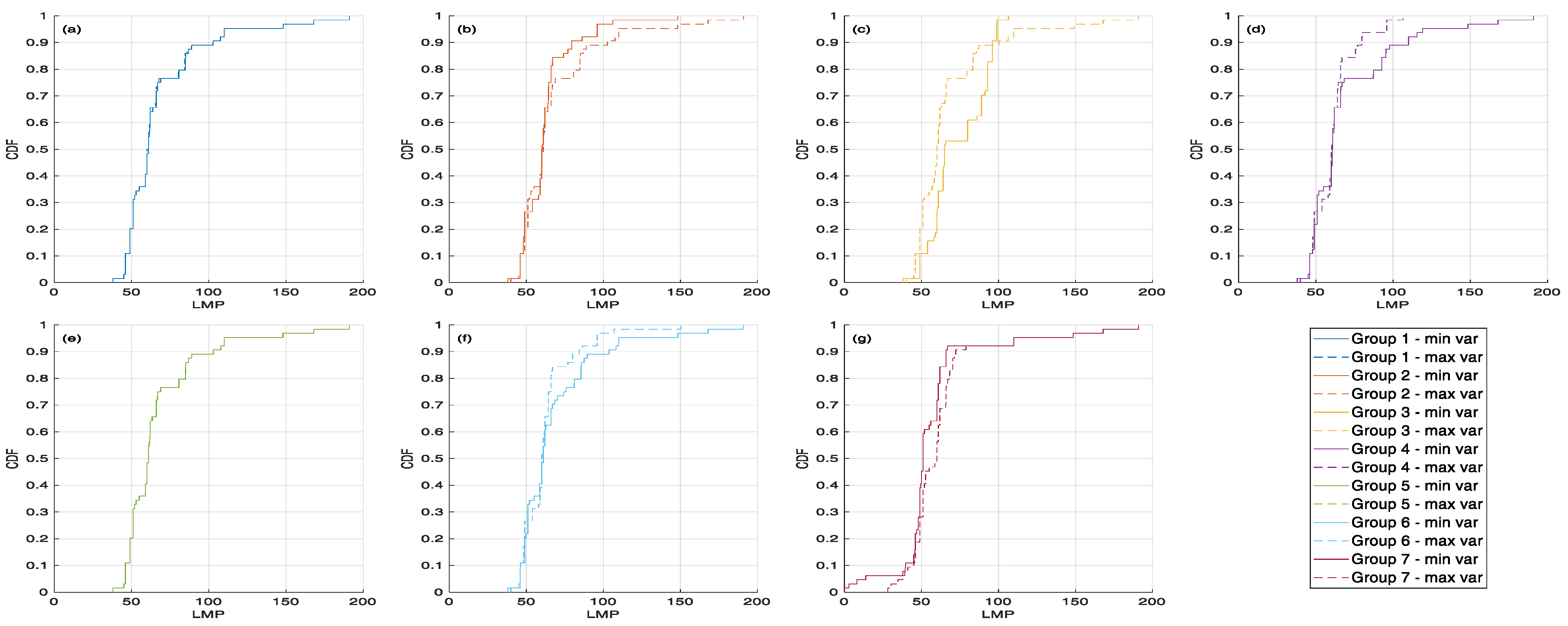
The Locational Marginal Prices (LMPs), which provide the information on the nodal prices. The LMPs are the nodal variables mostly used in the literature for the definition of the bidding zones [11]. The congestion that could appear in the network affects the differences among the LMPs determined for the nodes. The LMPs are calculated by executing the Optimal Power Flow (OPF), taking the Lagrange multipliers associated with the power balance equality constraint, and with the inequality constraints referring to the network security.
(2)
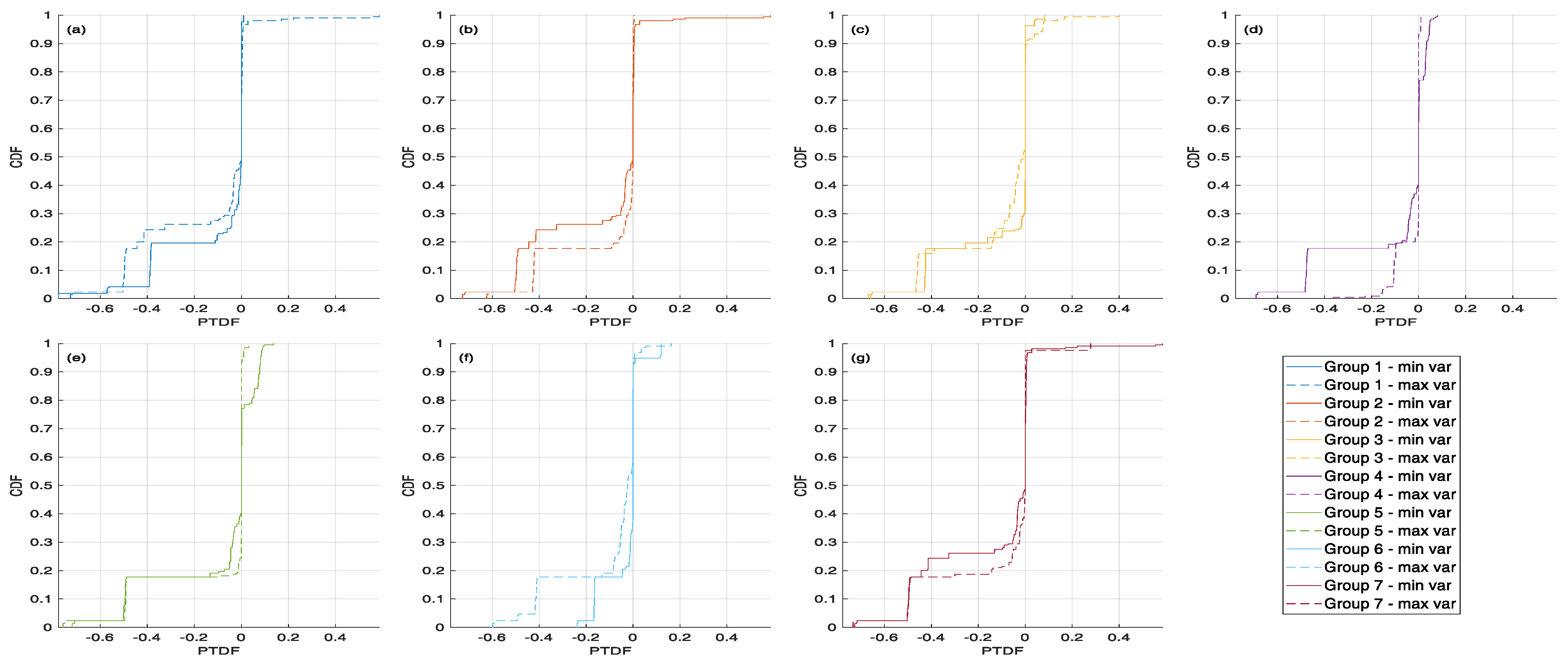
The Power Transfer Distribution Factors (PTDFs), which represent the sensitivity of the power flow in a connection due to the variation of the power injected in a node.
For each scenario, a “Direct Current” Optimal Power Flow (DCOPF) that explicitly incorporates the N-1 security criteria has been run to compute realistic LMPs and PTDFs, which depend on the load and generation profiles [12]. Furthermore, the TSO assigned a weight to each scenario, to represent its relative importance (e.g., probability of occurrence estimated according to historical data).

3. Application of Clustering Methods to Form the Bidding Zones

3.1. Overview on the Clustering Methods Applied to the Formation of the Bidding Zones and Related Challenges

The output of the BZ formation process is the classification of the electrical nodes of a transmission network into clusters. Each resulting zone must constitute an electrically connected subset of the grid where market participants are able to exchange energy without violating the line transmission limits [13].
Different clustering methods have been applied to the formation of the bidding zones [14]. In unsupervised approaches such as k-means and hierarchical clustering (HC), the metrics used are mostly based on the Euclidean distances. Penalty factors can be defined for penalising the distances between pairs of nodes not connected to each other.
In previous contributions, the authors of this paper have presented various results obtained from the application of clustering methods to form the bidding zones. A summary of these results is reported below.
The first aspect refers to the applicability of the basic versions of the clustering algorithms, as the ones that can be found in tools like MATLAB®. Most of these algorithms are inappropriate to determine suitable bidding zones, because there is no consideration of the network topology. As a result, solutions based for instance on LMPs could group together nodes located in different territorial areas, with no connection among these areas. Thereby, these methods cannot be used as they stand. The idea of carrying out post-processing of the results to connect the areas is unfeasible, because of the scattered location of the nodes belonging to the same group, with no physical connection among the nodes. On the other hand, in a post-processing it would be possible to identify more clusters by grouping together various groups of connected nodes previously included in the same cluster. However, in this case the final number of clusters could increase considerably, also forming groups with a very small number of nodes, thus inappropriate for being considered as a bidding zone [15].
Customisation of the clustering algorithms can be carried out, with the aim to introduce an internal check of the interconnections during the execution of the clustering procedure. In this case, it is possible to either exclude the merging of groups that do not contain any connected pairs of nodes between the groups, or to incorporate some penalty factors in the calculation of the distances between nodes, with the objective of discouraging the merging of groups when there is no interconnection among their nodes. With these modifications, the final number of clusters can remain the same as the initial one, and this can be useful for the execution of clustering methods that require the number of clusters as an input data.
The solutions obtained highly depend on the clustering method adopted. Even some variants of the same method can lead to very different results. This has been shown in [14] for four variants of the customised agglomerative HC algorithm, based on Euclidean distance, in which the only difference has been the linkage criterion adopted. Taking two groups of nodes, the linkage criterion determines how to calculate the distance between the two groups [16]. Using classical linkage criteria such as single, average, and Ward [17], the results obtained with the same number of bidding zones were significantly different. The single linkage criterion created a big cluster and had the trend of isolating some outliers. The Ward linkage criterion again led to the creation of highly populated clusters and a few smaller clusters. The average linkage criterion created more uniform partitions. These results are in line with other applications of the linkage criteria [18].
Another solution to improve clustering accuracy by adding knowledge on the problem domain has been suggested in [19], by considering clustering algorithms based on graphs, in particular by introducing specific constraints into the k-means algorithm [20]. Two types of constraints have been introduced, namely, (i) must-link constraints (e.g., pairs of nodes that must belong to the same cluster based on previously known information), ad (ii) cannot-link constraints (e.g., pairs of nodes that cannot belong to the same cluster based on previously known information). In the modified version of k-means developed in [19], called COP-kmeans, each component (e.g., node in the case of our paper) is assigned to the closest cluster that does not violate the constraints, and the absence of available clusters results in clustering failure. However, the introduction of the constraints referring to the domain knowledge changes the basic rationale of the clustering algorithms, with consequences on the computation times and convergence characteristics that depend on the effect of the constraint. On the other hand, the introduction of the constraints can make clustering performance less sensitive to the algorithm chosen, especially when the constraints (e.g., on network topology) drive the solution in specific directions.
The application of must-link and cannot-link concepts has been used in some problems referring to electrical networks such as the formation of intentional islands [21], in which the relations between nodes belonging or not to an island is known a priori. However, these concepts cannot be directly incorporated in the clustering algorithms aimed at creating the bidding zones, because the previous information only concerns the network topology, while there is no pre-established decision referring to the location on pairs of nodes within the same cluster or in different clusters. In Chapter 7 of the book [22], the discussion that mentions the existence of constrained clustering algorithms indicates the possibility of accommodating contiguity constraints to ensure that the clusters form connected sub-graphs, adding “while we did not encounter such problems in practice”. The problem under consideration in this paper requests the presence of connected sub-graphs in each cluster, thus indicating how the studies in progress address challenging aspects in the clustering domain.
In the next subsection, a novel procedure is proposed to identify the bidding zones, considering both the topological constraints and the features that characterise the nodes of the network.

3.2. General Aspects of the Proposed Procedure and Notation

The input data available refer to the network structure, the selected scenarios and the corresponding selected features. The general notation is indicated below.
(a)
Variables:
DNumber of LMP and PTDF initial data for each bus
FNumber of input features for clustering (LMP or PTDF). If the input features are LMPs, it corresponds to FLMP. If the input features are PTDFs, it is equal to FPTDF
FLMPNumber of LMP input features for clustering
FPTDFNumber of PTDF input features for clustering
KNumber of centroids
NNumber of nodes
LNumber of lines
SNumber of types of scenarios
(b)
Vectors and matrices:
A    N , N Node adjacency matrix
DLMP   N ,   D Initial LMP data matrix
DPTDF   N ,   D ,   L Initial PTDF data matrix
P   N , N Similarity matrix
X    N , F Input data matrix for clustering
v    N , 1 Cluster location vector
w    S , 1 Vector containing the weighting factors for the scenarios

3.3. Input Data Pre-Processing in the Multi-Scenario Clustering

The node adjacency matrix A contains the connection among all pairs of nodes, coded in binary form (0 = not connected; 1 = connected). The nodes are defined in such a way to represent all the possible interconnections of the busbars inside the power substation (i.e., multiple nodes are used to represent separate operation of the busbars in different scenarios). However, the matrix A does not change in all the calculations carried out for clustering. Possible situations in which one of the nodes (e.g., a busbar) is not connected to the rest of the system are handled by assigning to this node the same LMP of the node corresponding to the other busbar in the substation.
The presence of multiple scenarios is firstly addressed by forming a set of features, which are LMPs and PTDFs for each scenario and node. In this way, the data input vectors with LMPs and PTDFs are formed as two data matrices: DLMP and DPTDF. The first one is a 2-D array, while the second is a 3-D matrix, since PTDFs involve the branch elements as well. For both of them, the row and the column indices are associated to the node identifier and to the scenario identifier, respectively. The third-dimension index of DPTDF represents the branch identifier. For the sake of uniformity, DPTDF was reshaped in a 2-D array, horizontally concatenating the PTDFs that are related to the same scenario. For PTDFs, only the congested lines have been considered, in line with the CBCO principle.
In order to reduce the computational time, the columns in which all the considered features (LMPs or PTDFs) are equal have been eliminated, as they would not contribute to the calculation of the distances between nodes in the clustering procedure. In this way, the input data used for clustering is included in the matrix X, with the number of columns equal to the number of features F. The elimination of the columns with all equal entries could be an issue if the number of remaining columns becomes too small. In this case, the meaning of the results could be affected, depending only on a small number of entries. This point has to be checked in advance by considering the input data. Even though there is no specific threshold to apply to the minimum number of columns to be used, the interpretation of possible issues with the results depending on the number of columns is mainly provided by the expertise of the TSO.

3.4. Multi-Scenario Clustering Methodology

The node grouping should be carried out evaluating both the intra- and the inter-scenario distributions of the considered features.
The rationale of the novel approach shown in this paper is based on the following requirements:
  • The bidding zones shall be formed by only interconnected buses.
  • Nodes that always belong to the same cluster should be part of the same bidding zone.
  • Scenarios with more likelihood of occurrence should have greater impact.
  • The number and the likelihood of occurrence of the scenarios are not rigid constraints.
These requirements are accomplished by an approach that requires the execution of three steps, summarized in Figure 3.
(1)
In the first step, a clustering algorithm is executed by considering each scenario individually (the algorithms used in this paper are listed in Table 2).
(2)
In the second step, for each pair of nodes, a similarity index is computed on the base of two factors, as shown in Equation (1) for the nodes i and j: (i) the number of times in which the selected nodes belong to the same clusters, and (ii) the likelihood of occurrence of each scenario.
p i , j = f = 1 F p f P F k f
where:
  • p i , j is the similarity index for the nodes i and j;
  • p f is the probability of occurrence of the scenario related to the feature f;
  • P F = f = 1 F p f ;
  • k f = { 1 F ,   if   the   node   i   and   j   belong   to   the   same   clusters   for   the   considered   scenario 0 ,   otherwise  
The indices are collected in the symmetric similarity matrix P, which is a matrix representation of a similarity graph. A value P i , j = 0 means that the nodes i and j of the similarity graph are not connected.
(3)
In the third step, with P as input, the nodes are merged into the desired number of groups running a graph-based clustering algorithm (this paper uses Spectral Clustering [23], with the number of groups as the single input parameter), which allows to handle the topology constraints. Spectral clustering has been applied in to determine areas in the power system on the basis of specific properties (e.g., admittance matrix [24] power flows and line admittances [25], both without referring to the bidding zone formation). In [25], spectral clustering has been used by considering branch-based attributes, taken from the line admittances, as the first stage of the calculations, and has been followed by a second clustering method (with hierarchical clustering). In [26], the spectral clustering has been combined with k-means for determining bottlenecks on the transmission system. In the approach proposed in this paper, the spectral clustering is used as the last step, conversely to what happens in other approaches.

4. Applications and Results

The clustering methodology reported in the previous section, developed to manage scenario-based LMP and PTDF data, is adopted to analyse the Italian network case study.

4.1. Italian Network Data

The Italian transmission network is composed of an interconnected set of nodes located in all of the Italian regions. The network is also interconnected with the neighbouring countries of continental Europe (France, Switzerland, Austria and Slovenia), and with other countries or territories (Greece, Montenegro, the Corsica island in France, and Malta) through submarine links.
For the purpose of the study carried out in this article, the island of Sardinia is considered as an individual bidding zone, being a different synchronous area, and is then excluded from the computations. The nodes at the external interconnections are excluded as well. Hence, the network nodes considered include the continental part of Italy and the Sicily island. The network model has 918 nodes and 1317 branches. Five types of scenarios are considered, in which the weights depend on the historical occurrence of the planned outages (and of similar ones) [12]. Table 1 recalls the characteristics of these types of scenarios, with the weights established by the TSO and the specific indication. In particular, the outages indicated for the scenario types S1 and S2 limit in a significant way the transmission capacity in the south-north interconnections and from the south to the central part of Italy, respectively. The outages indicated for the scenario types S3 and S4 do not impact the transmission capacity between existing bidding zones in a significant way, however in the latter case intra-zonal congestions could occur during this unavailability. In the scenario type S5 the TSO weight is the difference between 100% and the sum of the weights of the other scenarios. The input data of the BZ formation process are the LMPs and the PTDFs, considered separately. These features were preliminary calculated from an optimal DC power flow [12].

4.2. Input Data and Preliminary Analysis

The initial set of data includes D = 100 initial data for each node, taken from the 5 types of scenarios. The input data matrices have been pre-processed as described in Section 3.3. In particular, the columns (i.e., the scenario) of the matrix DLMP with a unique LMP value for all the rows (i.e., the nodes) have been deleted in order to reduce the computational time, as they would not contribute to the computation of the distances between nodes in the clustering procedure. After the column elimination, the number of rows and columns of the remaining input data matrix that it has been processed by clustering algorithms is N = 918 nodes and FLMP = 65 features, respectively. Similarly, concerning PTDF, only data related to congested lines are extracted from the original matrix DPTDF. The number of rows and columns of the matrix processed by clustering algorithms is N = 918 nodes and FPTDF = 214 features, respectively.
The input data matrices for clustering have been statistically analysed, computing the mean values and the variance of the features. Figure 4 and Figure 5 show these values for each node for LMPs and PTDFs, respectively. The colour of the bubbles is representative of the mean values, while the size indicates the variance. From this preliminary analysis, the LMP mean values in a certain area look more homogenous than those related to PTDFs. Moreover, according to the size of the bubbles, it seems that the variance of PTDFs is higher than that of LMPs. More insights are provided from the plot of the cumulative distribution functions (CDFs) of the LMPs (Figure 6) and PTDFs (Figure 7), for an illustrative example with 7 groups. In particular, the lack of smoothness in the CDFs reflects the presence of the planned maintenance cases indicated in Figure 2, which change the levels of LMPs and PTDFs. The results shown in Figure 4 and Figure 5 could prefigure a partitioning into clusters. However, the probability distributions of the features are rather far from normal distributions, and large variances appear in some nodes, thus requesting further analyses before reaching appropriate conclusions on the bidding zone selection.

4.3. Results of the Clustering Procedures

At first, the k-means and spectral clustering are executed alone to remark some critical aspects of their application. Figure 8 shows the results of the bidding zone formation process using LMPs or PTDFs as features, with the formation of 7 clusters (equal to the number of bidding zones in the current configuration). Each BZ is marked with a different colour. The main drawback is the creation of clusters of different sizes, also of very small size. All these solutions could be considered not appropriate for the purpose of determining the bidding zones. This justifies the formulation of a more suitable approach, as the one presented in this paper.
The procedure described in Section 3.4 is then executed by considering different types of input data (LMPs and PTDFs) and different settings. In particular, three clustering algorithms were tested within the step 1 of the process visible in Figure 3, that are the hierarchical clustering with the average linkage (HC-A), with the single linkage (HC-S) and k-means (KM). Moreover, the number of clusters was changed in the range of 2 to 7, in a way consistent with the number of bidding zones existing in the corresponding part of Italy (six zones, as the island of Sardinia, which is depicted in Figure 1, has been excluded from the analysis). A first promising result is that, for a given number of clusters provided as input, the solutions are nearly the same for all the tested clustering algorithms and all the features. For the sake of brevity, as an example, Figure 9 depict the solutions identified for the different numbers of desired clusters provided as input. Each BZ is marked with a different colour. They were computed considering LMPs as features, and HC-average as the clustering algorithm executed in the step 1 of the process (Figure 3). Looking at the sequence of the figures, it is possible to discover a consistent path with which successive partitions are formed. The Sicily island remains always associated to the same separate group. The central and southern parts of Italy remain in the same group (with small differences) up to 6 groups (including some nodes located in the current center-north zone of Figure 1), while a partitioning into two groups (different from the current partition indicated in Figure 1) appears with seven groups. The major changes appear in the northern part of Italy. The first split occurs from three to four groups, then with five groups a small group appears in the northwestern part, which becomes larger passing to six and seven groups. Another partition is found on the northeastern part when six groups are formed and remains passing to seven groups. It is important to remember that these results are based on historical datasets (e.g., expected investments in the coming years are not considered in the current simulations) and the set of scenarios to be considered should be enlarged before drawing any conclusion and comparison to the existing bidding zone configuration.
As expected, the higher the number of desired groups, the higher the fragmentation of the solution. With seven clusters, the two smallest groups are formed by 74 and 44 nodes. These numbers of nodes are in principle reasonable to be considered in the process of formation of the bidding zones.
Another aspect that has been investigated is the effect of changing the clustering algorithm in the first stage of the proposed approach (step 1 in the flowchart of Figure 3). Figure 10 shows the results obtained by executing the three clustering algorithms indicated in Table 2, in each case followed by the same spectral clustering algorithm. From these results, a major advantage of the proposed procedure emerges: the solutions obtained are quite similar regardless of the clustering algorithm used in the initial stage. The proposed approach is then satisfactorily robust with respect to this choice.
In addition, the solutions remain similar also in spite of the different probability distributions of the LMPs and PTDFs shown in Section 4.2. This is a further confirmation of the benefits of applying the proposed multi-stage approach.

4.4. Assessment of the Clustering Solutions

Performance assessment is a relevant aspect for a clustering-based study. In general, many clustering validity indicators are available from the literature to assess the quality of the clustering results. However, there is a key point to consider: the calculation of a clustering validity indicator requires only the data on the initial features and the vector that contains the indication on the cluster in which each node has been located. In our case, the clustering procedure also depends on the node connection, besides the features. The information about the node connection is not directly represented in the calculation of the clustering validity indicators, making the results questionable. Further work is needed to establish suitable clustering validity indicators that are appropriate for assessing the quality of the results in the specific case.
For the sake of comparison, being aware of the limitations discussed above, we have applied some clustering validity indicators taken from the literature, comparing the results obtained with LMPs and PTDFs as features. The results obtained by using the Clustering Dispersion Indicator (CDI) [27] are presented as an example. A key aspect in this case is that the results obtained by calculating the clustering validity indicators with the use of different features can be compared only when the same features are used to represent the initial data as the “common ground”.
In particular, taking the LMPs as the “common ground”, the clustering validity indicators are calculated by using the vectors that contain the cluster in which each node has been located in both cases of using the LMPs or the PTDFs as features (Figure 11a). Then, taking the PTDFs as the “common ground”, the clustering validity indicators are calculated by using the same vectors that contain the cluster in which each node has been located in both cases of using the LMPs or the PTDFs as features (Figure 11b). The main result is that the clustering validity indicators, calculated by using either the LMPs or the PTDFs as the “common ground”, provide similar results. This confirms the effectiveness of our approach in providing consistent results by using the two features.
It is also crucial to remember that, according to the current EU legislation [4], the quality of the proposed bidding zone configurations will have to be compared in the second step of the bidding zone review process where a long list of criteria have to be considered.

5. Concluding Remarks

This paper has extended the application of clustering algorithms for the purpose of grouping together the network nodes with similar evolution in time of the relevant features (LMPs and PTDFs) considering a dataset based on weighted scenarios that represent different operating conditions of the Italian power system. Five network topological conditions have been considered. The scenarios have been selected in order to account for different load and distributed generation conditions experienced in the power system.
The nature of the problem was not directly tractable with conventional clustering algorithms, due to the needs of considering the physical links among the network nodes and of guaranteeing the connectivity of the nodes in the resulting clusters. For this purpose, a specific multi-stage clustering procedure was designed and implemented. In this procedure, different clustering algorithms have been tested in the first stage, while the same spectral clustering algorithm has been executed in the final stage, to maintain the connection among the nodes belonging to each final group formed. The cases presented refer to a number of groups from three to seven, where the maximum number is consistent with the number of current Italian bidding zones.
From the results obtained, it is possible to formulate some general and specific considerations. The procedure provides similar results considering both LMPs and PTDFs as input features. Moreover, the procedure seems to be not sensitive to the choice of the clustering algorithm adopted in the first stage to group nodes within each scenario.
This article has presented the proposed clustering algorithms and the evolution of the solutions when the number of groups provided as input to the proposed procedure changes. In fact, it is important to emphasize that there is a conceptual difference between the clustering outcomes and the final bidding zones. The clustering outcomes provide the view on the node partitioning based on the features used and the constraints imposed. To define the final bidding zones, more contents such as the provision of reserves, relations with ancillary service markets, and market power issues have to be considered by the decision-maker. From a broader view, also uncertainty aspects on availability of generation and transmission could be taken into account. For this reason, the choice of the final number of bidding zones requires careful evaluations considering benefits and costs and is beyond the scope of presentation. Future work includes the development of a methodology to rank the identified solutions and support the decision makers in reviewing the actual bidding zones.

Author Contributions

All authors contributed to conceptualization, methodology, validation, formal analysis, investigation, writing and supervision. All authors have read and agreed to the published version of the manuscript.

Funding

This research was funded by Terna within the Ensiel research project “Specifica tecnica sulle metodologie model-based per la definizione di strutture zonali alternative” (ST159).

Conflicts of Interest

The authors declare no conflict of interest.

References

  1. Wolak, F.A. Measuring the Benefits of Greater Spatial Granularity in Short-Term Pricing in Wholesale Electricity Markets. Am. Econ. Rev. 2011, 101, 247–252. [Google Scholar] [CrossRef] [Green Version]
  2. Joskow, P.L. Challenges for wholesale electricity markets with intermittent renewable generation at scale: The US experience. Oxf. Rev. Econ. Policy 2019, 35, 291–331. [Google Scholar] [CrossRef]
  3. Pototschnig, A. The Importance of a Sound Bidding-Zone Review for the Efficient Functioning of the Internal Electricity Market; FSR Energy—Florence School of Regulation; European University Institute: Florence, Italy, 2020. [Google Scholar]
  4. European Commission. Commission Regulation (EU) 2015/1222 of 24 July 2015 Establishing a Guideline on Capacity Allocation and Congestion Management; European Commission: Brussels, Belgium, 2015. [Google Scholar]
  5. European Commission. Regulation (EU) 2019/943 of the European Parliament and of the Council of 5 June 2019 on the Internal Market for Electricity; European Commission: Brussels, Belgium, 2019. [Google Scholar]
  6. ARERA. Decision 496/2017/R/EEL “Disposizioni in Merito Alla Revisione Della Suddivisione Della Rete Rilevante in Zone”. ARERA. 2017. Available online: https://www.arera.it/it/docs/17/496-17.htm (accessed on 10 May 2021).
  7. ARERA. Decision 103/2019/R/EEL “Ulteriori Disposizioni in Merito Alla Suddivisione Della Rete Rilevante in Zone, in Esito al Processo di Revisione Svolto ai Sensi Del Regolamento (UE) 2015/1222 (CACM)”. ARERA. 2019. Available online: https://www.arera.it/it/docs/19/103-19.htm (accessed on 10 May 2021).
  8. ARERA. Decision 386/2018/R/EEL “Disposizioni in Merito Alla Suddivisione Della Rete Rilevante in Zone, in Esito al Processo di Revisione Svolto ai Sensi Del Regolamento UE 2015/1222 (CACM)”. ARERA. 2018. Available online: https://www.arera.it/it/docs/18/386-18.htm (accessed on 10 May 2021).
  9. Colella, P.; Mazza, A.; Bompard, E.; Chicco, G.; Russo, A.; Carlini, E.M.; Caprabianca, M.; Quaglia, F.; Luzi, L.; Nuzzo, G. Model-based identification of alternative Bidding Zone Configurations from Clustering Algorithms applied on Locational Marginal Prices. In Proceedings of the 2020 55th International Universities Power Engineering Conference (UPEC), Torino, Italy, 1–9 September 2020. [Google Scholar]
  10. Wood, A.J.; Wollenberg, B.F. Power Generation, Operation, and Control, 2nd ed.; Wiley-Interscience: New York, NY, USA, 1984. [Google Scholar]
  11. Chicco, G.; Colella, P.; Griffone, A.; Russo, A.; Zhang, Y.; Carlini, E.M.; Caprabianca, M.; Quaglia, F.; Luzi, L.; Nuzzo, G. Overview of the Clustering Algorithms for the Formation of the Bidding Zones. In Proceedings of the 2019 54th International Universities Power Engineering Conference (UPEC), Bucharest, Romania, 3–6 September 2019; pp. 1–6. [Google Scholar]
  12. Bovo, C.; Ilea, V.; Carlini, E.M.; Caprabianca, M.; Quaglia, F.; Luzi, L.; Nuzzo, G. Optimal computation of Network indicators for Electricity Market Bidding Zones configuration. In Proceedings of the 2020 55th International Universities Power Engineering Conference (UPEC), Torino, Italy, 1–9 September 2020; pp. 1–6. [Google Scholar]
  13. First Edition of the Bidding Zone Review—Final Report. 2018. Available online: https://eepublicdownloads.entsoe.eu/clean-documents/news/bz-review/2018-03_First_Edition_of_the_Bidding_Zone_Review.pdf (accessed on 10 May 2021).
  14. Michi, L.; Quaglia, F.; Bompard, E.; Griffone, A.; Bovo, C.; Carlini, E.M.; Luzi, L.; Chicco, G.; Mazza, A.; Ilea, V.; et al. Optimal Bidding Zone Configuration: Investigation on Model-based Algorithms and their Application to the Italian Power System. In Proceedings of the 2019 AEIT International Annual Conference (AEIT), Florence, Italy, 18–20 September 2019; pp. 1–6. [Google Scholar]
  15. Griffone, A.; Mazza, A.; Chicco, G. Applications of clustering techniques to the definition of the bidding zones. In Proceedings of the 2019 54th International Universities Power Engineering Conference (UPEC), Bucharest, Romania, 3–6 September 2019; pp. 1–6. [Google Scholar]
  16. Anderberg, M.R. Cluster Analysis for Applications; New York Academic Press: New York, NY, USA, 1973. [Google Scholar]
  17. Ward, J.H., Jr. Hierarchical grouping to optimize an objective function. J. Am. Stat. Assoc. 1963, 58, 236–244. [Google Scholar] [CrossRef]
  18. Chicco, G. Overview and performance assessment of the clustering methods for electrical load pattern grouping. Energy 2012, 42, 68–80. [Google Scholar] [CrossRef]
  19. Wagstaff, K.; Cardie, C.; Rogers, S.; Schroedl, S. Constrained k-means clustering with background knowledge. In Proceedings of the 18th International Conference on Machine Learning, Boca Raton, FL, USA, 16–19 December 2001; Volume 1, pp. 577–584. [Google Scholar]
  20. MacQueen, J. Some methods for classification and analysis of multivariate observations. In Proceedings of the 5th Berkeley Symposium on Mathematical Statistics and Probability; University of California Press: Oakland, CA, USA, 1967; Volume 1, pp. 281–297. [Google Scholar]
  21. Esmaeilian, A.; Kezunovic, M. Prevention of power grid blackouts using intentional islanding scheme. IEEE Trans. Ind. Appl. 2016, 53, 622–629. [Google Scholar] [CrossRef]
  22. Fouss, F.; Saerens, M.; Shimbo, M. Algorithms and Models for Network Data and Link Analysis; Cambridge University Press: Cambridge, UK, 2016. [Google Scholar]
  23. Von Luxburg, U. A tutorial on spectral clustering. Stat. Comput. 2007, 17, 395–416. [Google Scholar] [CrossRef]
  24. Hamon, C.; Shayesteh, E.; Amelin, M.; Sӧder, L. Two partitioning methods for multi-area studies in large power systems. Int. Trans. Electr. Energy Syst. 2015, 25, 648–660. [Google Scholar] [CrossRef]
  25. Sánchez-García, R.J.; Fennelly, M.; Norris, S.; Wright, N.; Niblo, G.; Brodzki, J.; Bialek, J.W. Hierarchical spectral clustering of power grids. IEEE Trans. Power Syst. 2014, 29, 2229–2237. [Google Scholar] [CrossRef] [Green Version]
  26. Cao, K.-K.; Metzdorf, J.; Birbalta, S. Incorporating power transmission bottlenecks into aggregated energy system models. Sustainability 2018, 10, 1916. [Google Scholar] [CrossRef] [Green Version]
  27. Chicco, G.; Napoli, R.; Postolache, P.; Scutariu, M.; Toader, C. Customer characterization options for improving the tariff offer. IEEE Trans. Power Syst. 2003, 18, 381–387. [Google Scholar] [CrossRef]
Figure 1. Present bidding zones in Italy and external interconnections. Reprint with permission [5056090322801]; 2021, IEEE.
Energies 14 02763 g001
Figure 2. Location of the planned maintenance cases.
Energies 14 02763 g002
Figure 3. Flowchart of the proposed multi-scenario clustering methodology.
Energies 14 02763 g003
Figure 4. The colour and the size of the bubbles represent the mean value and the variance of the LMP of a node, respectively.
Energies 14 02763 g004
Figure 5. The colour and the size of the bubbles represent the mean value and the variance of the PTDF for a node, respectively.
Energies 14 02763 g005
Figure 6. Cumulative Distribution Function (CDF) of the LMPs computed for the two nodes with the highest and the lowest LMP variance, for each one of the 7 groups shown in Figure 4. In particular, subfigure (a) refers to group 1, LMPs   [48, 52), subfigure (b) refers to group 2, LMPs   [52, 56), subfigure (c) refers to group 3, LMPs   [56, 60), subfigure (d) refers to group 4, LMPs   [60, 64), subfigure (e) refers to group 5, LMPs   [64, 68), subfigure (f) refers to group 6, LMPs   [68, 72), subfigure (g) refers to group 7, LMPs   [72, 76].
Energies 14 02763 g006
Figure 7. Cumulative Distribution Function (CDF) of the PTDFs computed for the two nodes with the highest and the lowest PTDF variance, for each one of the seven groups shown in Figure 5. In particular, subfigure (a) refers to group 1, PTDFs   [−0.16, −0.136), subfigure (b) refers to group 2, PTDFs   [−0.136, −0.112), subfigure (c) refers to group 3, PTDFs   [−0.112, −0.088), subfigure (d) refers to group 4, PTDFs   [−0.088, −0.064), subfigure (e) refers to group 5, PTDFs   [−0.064, −0.04), subfigure (f) refers to group 6, PTDFs   [−0.04, −0.016), subfigure (g) refers to group 7, PTDFs   [−0.016, 0.008].
Energies 14 02763 g007
Figure 8. Solution with seven clusters obtained through: (a) k-means, LMPs; (b) k-means, PTDFs; (c) spectral clustering, LMPs; (d) spectral clustering, PTDFs. The scenarios are not weighted.
Energies 14 02763 g008
Figure 9. Results for different number of clusters. The considered features are LMPs. The clustering algorithm adopted to group nodes within each scenario is HC-average. Subfigure (a) depicts the solution for 2 clusters, subfigure (b) for 3 clusters, subfigures (c) for 4 clusters, subfigures (d) for 5 clusters, subfigures (e) for 6 clusters, and subfigure (f) for 7 clusters.
Energies 14 02763 g009
Figure 10. Comparison of the solutions with seven clusters obtained with the algorithm/feature pairs: HC-average/LMPs (on the left) and KM/PTDFs (on the right).
Energies 14 02763 g010
Figure 11. Clustering Dispersion Indicator (CDI) computed considering LMPs (a) and PTDFs (b) as “common ground”.
Energies 14 02763 g011
Table 1. Types of scenarios [9].
Scenario TypeTSO WeightOperation or Outage
S15%Planned outage of a 380 kV line on the Adriatic path
S240%Planned outage of a 380 kV line in the southern part of Italy
S35%Planned outage of a 380 kV line in the central part of Italy
S420%Planned outage of a 380 kV line in the northwestern part of Italy
S530%all network elements are considered fully available
Table 2. Clustering algorithms adopted to group nodes within each scenario.
Clustering AlgorithmLinkage CriterionAcronym
HierarchicalAverageHC-average
HierarchicalSingleHC-single
k-means KM
Publisher’s Note: MDPI stays neutral with regard to jurisdictional claims in published maps and institutional affiliations.

