Linear Induction Motors in Transportation Systems

Abstract

This paper provides an overview of the Linear Transportation System (LTS) and focuses on the application of a Linear Induction Motor (LIM) as a major constituent of LTS propulsion. Due to their physical characteristics, linear induction motors introduce many physical phenomena and design constraints that do not occur in the application of the rotary motor equivalent. The efficiency of the LIM is lower than that of the equivalent rotary machine, but, when the motors are compared as integrated constituents of the broader transportation system, the rotary motor’s efficiency advantage diminishes entirely. Against this background, several solutions to the problems still existing in the application of traction linear induction motors are presented based on the scientific research of the authors. Thus, solutions to the following problems are presented here: (a) development of new analytical solutions and finite element methods for LIM evaluation; (b) comparison between the analytical and numerical results, performed with commercial and self-developed software, showing an exceptionally good agreement; (c) self-developed LIM adaptive control methods; (d) LIM performance under voltage supply (non-symmetrical phase current values); (e) method for the power loss evaluation in the LIM reaction rail and the temperature rise prediction method of a traction LIM; and (f) discussion of the performance of the superconducting LIM. The addressed research topics have been chosen for their practical impact on the advancement of a LIM as the preferred urban transport propulsion motor.

1. Introduction

A traction Linear Induction Motor (LIM) has been deployed worldwide in numerous transit systems and in driverless, elevated guideway systems requiring all weather operations under very short headways. LIM-based urban transport has proven to be, by far, the least expensive in terms of operations and maintenance (including the energy costs). LIMs are also found in other various applications, ranging from small-power industrial material handling and amusement park roller-coaster propulsion to very high-output military aircraft launchers; advanced research is underway to investigate LIMs as potential power conversion devices for ocean wave energy recovery [1].

Because of low operating costs and extremely high reliability, LIM-propelled systems have become an ever more frequent part of the public transport offering. LIM-based public transit systems have already been in operation for a few decades, and they are serving such cities as Yokohama, Vancouver, Toronto, Tokyo, Osaka, Seoul (Yongin), New York, Moscow (Moscow Monorail), Kuala Lumpur, Guangzhou, Fukuoka, and Beijing. References for the applications are readily available by any browser search using such keywords as “Linear Metro”. For economic reasons, the operation of these systems as well as most other LIM-based systems has been based on a single-sided LIM [1,2]. Although, in comparison to its rotary counterpart, a traction LIM has necessarily a large air gap between the stator and its rotor equivalent and thus is less efficient on the motor-to-motor comparison bases, the LIM-based systems show better system-level performance resulting from several characteristic features specific to the LIMs. First, in comparison with rotary induction motors, a mechanical gear box that introduces high energy losses and accounts for a significant life cycle cost and is a potential source of serious reliability issues is eliminated. The LIM has no moving parts, and the propelling force is directly applied to the vehicle in the direction of motion, thus avoiding the losses introduced by the mechanical gear box. In most instances, rotary-motor-based transportation systems rely on adhesion between the wheels and the running rail. Relying on adhesion limits their acceleration and deceleration performance under wet or otherwise contaminated rail conditions. LIM systems do not suffer such disadvantages because their tractive effort is developed as a direct electrodynamic force between the LIM primary and the reaction rail, and this allows for an adhesion independent, reliable operation under all environmental conditions. This also means that LIM-propelled trains (objects) can accelerate at any rate and achieve their nominal speeds sooner, which limits the high current/tractive effort demand period and decreases the overall energy consumption. Because of their flat form, LIMs occupy significantly smaller vertical space, which enables a lower profile steerable bogie construction and, consequently, a lower vehicle cross-sectional area, thus decreasing the potential tunnel construction costs and energy consumption resulting from the motion air resistance [3,4]. In addition, LIM-based vehicles can run on steeper grades (due to direct forces) and negotiate sharper curves (due to steerable bogies), providing more flexibility in the elevated guideway structure design, which helps to reduce civil and land release costs. A large urban center allows for more targeted interconnection of the various multimodal transportation systems, which is not always achievable with rotary-motor-based rail vehicles. The uniqueness of Linear Motor (LM) systems led to a heightened interest in LIM technology and resulted in a number of research projects aimed at improving LIM performance and further decreasing the operating cost.

In this paper, an overview and categorization of linear transportation systems is completed, in which LIMs are found to mainly be used for traction and braking. Next, the major characteristics of a LIM are described and associated with the system performance. Finally, a series of important practical research works carried out by the authors and aimed at advancing LIM system performance are reported, highlighting challenges associated with improving LIM performance in such areas as performance prediction, LIM adaptive control, LIM thermal protection, and the application of superconductivity. The conclusions summarize the authors’ experience in the subject matter and highlight the areas of advancement for future research.

2. Overview of Linear Transportation Systems

Linear transportation systems (LTSs) can be divided into some fundamental groups according to their support, guidance, and drive solutions. The most important groups are listed below.

2.1. Levitated LTS

Levitated LTSs mainly use electromagnetic suspension. These systems, Maglevs, can be divided into Permanent Magnet (PM)- and superconductor-based levitating systems. According to the postulate on the stability of bodies in various static force fields given in 1842 by Earnshaw [5], no object placed in an inverse square law force field (e.g., magnetic field) could be in a stable equilibrium; thus to achieve stability, PM flux should be modulated by the respective control coil currents that depend on the size of the air gap. Such controlled electromagnets are utilized in many different levitation systems, for both side and vertical stabilization [6]. Efficient operation of these systems depends on the advanced optimization of the magnetic field distribution within the air gap by means of proper geometry design and proper selection of material and power supply characteristics [7,8].

The first Maglev line to open to public traffic was the Birmingham Maglev in 1984 (propelled by a LIM), the second was the M-Bahn in Berlin (also 1984), and the third was the Shanghai Transrapid Maglev (the latter two using a long-stator synchronous linear-motor-based propulsion).

Braunbeck [9] extended stability investigations to the systems containing diamagnetic materials. The characteristic feature of a diamagnetic material is that it opposes the external field variations, the feature exhibited by the superconductors. Since their inception, superconducting levitation systems have been used in many different industrial applications. The principle of these systems is based on the interaction between the magnetic field and high-temperature superconductors [10,11]. Two examples of superconducting levitation systems are the Miyazaki and Yamanashi Maglevs. In the early stages of Maglev development, at the Miyazaki test track (1977), a purely repulsive electrodynamic suspension system was used [12]. A major advantage of the repulsive electrodynamic suspension system is its inherent stability—a decreasing distance between the track and the vehicle results in strong reactive forces bringing the system to its original position. The magnetic field can be produced by either superconducting magnets (as in JR-Maglev) or an array of permanent magnets (as in Inductrack). The disadvantage of the electrodynamic suspension is that the repulsive forces are speed dependent and are low at low vehicle speeds. For this reason, the vehicle must use support wheels until it reaches take-off speed.

In [13], the hyperloop all-in-one advanced LIM system (propulsion, levitation, and guidance) was proposed. The Superconducting Transverse Flux Linear Motor with integrated levitation, guidance, and propulsion system was described in [14]. Another superconducting levitation system for linear drives was proposed in [15].

In 2015, an SC-Maglev train operated by the Central Japan Railway Company (JR Central) broke the train speed world record by clocking in at 603 km/h (374 mph); a new Chinese Maglev system intended for speeds up to 620 km/h was unveiled in January 2021 by CRRC in Chengdu.

2.2. Non-Levitated LTS

This type of LTS uses conventional wheels and is the most typical solution of linear transportation systems [1,16,17,18]. According to the electrical drive system, these linear transportation systems can be driven by DC motors and synchronous or induction motors—conventional or superconducting.

2.3. LTS with Synchronous Motors

Various levitated LTSs using conventional synchronous motors based propulsion were described in [19], e.g., they are permanent-magnet-excited machines. A high-temperature superconducting linear synchronous motor was described in [20]. The application of superconducting linear flux-switching permanent magnet motors was discussed in [21].

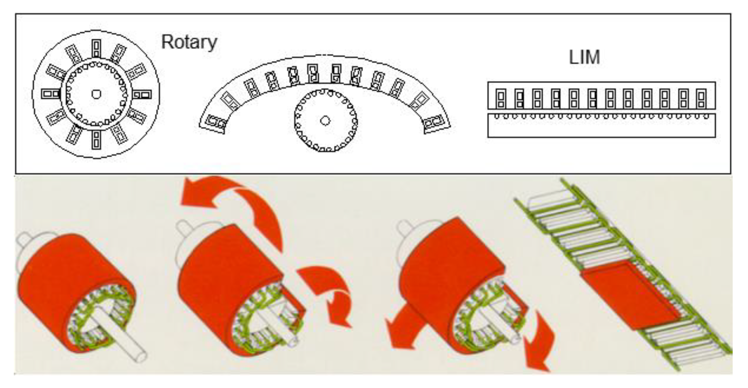
2.4. LTS with Induction Motors

Linear induction machines were discussed as the most promising solution for LTSs in [1,15,17,18]. In the late 1940s, the British electrical engineer Eric Laithwaite, Professor at Imperial College London, developed the first full-size working prototype of the linear induction motor. The first commercial Maglev transport system in the world, the Birmingham Maglev, which opened in 1984, was also propelled with a linear induction motor. The latest problems related to the application of LIMs are discussed in Section 3.

2.5. LTS with Superconducting Induction Motors

When it comes to LTSs, superconductivity can not only be used for levitation but also for generating a tractive effort [10,21,22,23,24,25,26]. Superconducting motors have their windings made of low-temperature, conventional, or high-temperature superconductors. A typical linear induction motor with an iron core and copper winding can produce only a limited thrust because of the flux saturation of the iron core. High-temperature superconducting windings can generate a strong magnetic field and, consequently, large thrust. High flux density and high thrust can be produced over a wide gap range because of extremely high ampere turns (see Section 4.5).

Some general problems connected with the electromagnetic fields related to high-speed LTSs driven by different linear motors (synchronous, induction, superconducting) were described in [27].

3. Linear Transportation Systems Using Induction Motors

A LIM can be obtained from its rotary counterpart, the induction motor, by an imaginary process of cutting the rotary’s stator and rotor in a radial plane and unrolling it, at the same time as replacing a cage or a winding with a conducting sheet, as in Figure 1.

Should the second primary be added to the single-sided LIM in Figure 1, a double-sided LIM would be formed. Depending on the relative length of the secondary and primary, the LIM can be categorized as a short-secondary (Figure 2) or a short-primary LIM.

The rotary motor can be thought of as “infinite” in that its primary winding generated magnetic field is continuous and has no beginning or end around its circumference. Unlike the rotary, the short-primary LIM has a finite length. Thus, only the part of the secondary side that is immediately below the primary is subjected to a primary generated magnetic field. During motion, the new unexcited parts of the secondary side equivalent “rotor” continually enter under the LIM primary magnetic field generated by a distributed Magnetomotive Force (MMF). This process generates a continuous electromagnetic response in the new incoming segments of the secondary, the Reaction Rail (RR), in a form of induced MMF, thereby resisting the immediate establishment of the magnetic flux under the front end of the LIM primary. Subsequently, the reaction rail MMF decays but at a lower rate dictated by the “rotor time constant” of the motor. Figure 3a shows a short-primary LIM, and Figure 3b shows the reaction rail. The RR consists of a series of aluminum top cap segments, connected for electric continuity, and underlying iron bars, the Back Iron (BI), corresponding to the conventional rotor winding and rotor laminations, respectively.

LIMs can be further classified into a number of other topologies, but so far only the single-sided, short-primary linear induction machine has been successfully used in urban transportation systems [1,2,15]. It seems to be a natural choice since the cost of building an active multiphase primary along a multikilometer guideway would render such systems uneconomical. In most existing urban applications, the primary is suspended under the bogie, over a track-installed reaction rail consisting of either solid or laminated mild steel BI covered with an aluminum extrusion supported on an assembly that permits the transfer of forces to the guideway. In most current applications, mainly in South-East Asia, Canada, and the USA, the guideway is of an elevated, right-of-way type requiring a minimal footprint and does not affect other modes of ground transportation.

As already mentioned, the relative motion between the finite-length primary and the infinite secondary induces a dynamic end effect by creating end-effect currents in the aluminum top cap that demagnetize the oncoming end of the motor. The currents produce additional forces and losses that exist even at synchronous speed and increase with vehicle velocity. The static end effect, another LIM-related phenomenon, occurs because of the phase impedance imbalance caused by the finite length of the phase winding. The effect is amplified by the dynamic end effect, which distorts the air-gap magnetic flux density, having a direct effect on the flux linked to the phase windings. The transverse edge effect is yet another phenomenon characteristic of LIMs. Its major source is the longitudinal component of the top cap induced current. The two major impacts of the transverse edge effect are an increase of the equivalent secondary resistance and an uneven flux distribution across the LIM’s primary. Because of the dynamics of the vehicle as well as the RR’s limited construction accuracy, the reaction rail is usually offset from the longitudinal symmetry line of the primary side of the LIM, leading to decentralized transverse forces and potential lateral instability. The asymmetrical construction of the reaction rail necessitated by the vicinity of switches aggravates this effect.

Many constraints exist in the high-speed urban electric traction LIM application, which requires a large distance between the LIM primary and the secondary side RR. Running rail and truck deflection, rail canting, and wheel wear are the major reasons for using a large air gap with the LIM. For a gap length of ten to fifteen millimeters, the ratio between the air-gap width and the pole pitch is significant and leakage flux is considerable. The values of up to 100 Hz are not uncommon in today’s applications of urban traction LIMs. At the operational slip of around 10–15%, the skin effect in the aluminum cap is not completely negligible. Finally, there are unbalanced normal forces, attractive and repulsive, that add additional complexity in the analysis of the optimal gap and the construction of the motor, as they affect the distance between the lowest point of the primary and the top of the reaction rail top cap.

Because of the differences between the LIM and the rotary machine, unconventional analysis techniques and modeling methods have been developed in an attempt to account for the number and magnitude of LIM-characteristic phenomena.

Many methods of LIM calculation, optimization, and control are identical (or very similar) with the methods applicable to rotating induction machines. The electromagnetic calculations of the rotary motor are reasonably simple because of the motor’s “infinite” character and the possibility of applying symmetry boundary conditions, thus limiting the solution region and speeding up the calculations even further. Two dimensional calculations assure sufficient accuracy for the performance prediction of a standard rotary motor. However, the LIM is not symmetrical. The phenomena occurring in the front end of the motor are different than in the receding end and therefore the symmetry boundaries cannot be used, which leads to longer calculation times.

3.1. Analytical Solutions Applied for the LIM Evaluation

LIMs are made of several major components such as the magnetic steel primary core, distributed three-phase copper winding with a three-phase excitation terminal, aluminum top cap, and magnetic BI. The primary is finely laminated and during LIM electromagnetic calculations, for simplicity, the conductivity of the primary can be set to zero. However, the BI conductivity cannot be assumed as zero because the BI is usually only coarsely laminated—mainly for economic reasons. Instead, for the case of the slab-shaped BI, the BI conductivity must be set to its true material value and a respectively lower value for the case of coarse laminations. This value of conductivity is usually determined based on matching the test LIM’s longitudinal performance with the simulation model results. Theoretical methods of assessing the BI conductivity have been proposed but, so far, they only serve as a guidance for the empirical derivation. Figure 4 shows the three-dimensional model of the LIM [29].

The development of analytical methods aimed at solving the LIM problems (separation of variables method, integral equations method) took place in the 1970s. Currently, the main method of analysis is Finite Element Analysis (FEA). Many recently published papers contain both analytical and numerical solutions, where the analytical calculations have mostly been made for validating the results of the numerical models.

Despite significant progress in numerical algorithm efficiency and modern computer speeds, the 3D simulation models of large LIMs are still prohibitively time consuming to solve. The following simplifying assumptions are usually made to the LIM to simplify the calculation process:

• A 2D analysis can be used;
• The iron magnetization curve is linear;
• The conductivity of the reaction rail is constant;
• Motion in the x-direction only is allowed.

The equation that describes the electromagnetic field distribution within the 2D LIM model has the following form:

$$\frac{{\partial }^{2}A}{\partial x^2}+\frac{{\partial }^{2}A}{\partial y^2}=\mathsf{\mu }(-J+j\mathsf{\omega }\mathsf{\sigma }A+\mathsf{\sigma }{v}_x\frac{\partial A}{\partial x})$$

(1)

where A is the z-component of the magnetic vector potential, J is the z-component of current density, ω is the angular frequency, v_x is the velocity in the x-direction, and σ and µ are the conductivity and permeability, respectively.

Analytical solutions for the evaluation of the LIM properties have been discussed in many papers. In most of them, the standard mathematical approach to LIM modeling is to define the currents of the primary windings as sinusoidally distributed current sheets [17,30,31,32,33,34,35].

Mathematical and experimental research of coils or filaments moving above a conducting plate (limited to DC excitation) were performed in the majority of the Maglev application studies [36,37,38,39,40]. The system of a stationary filament or coil with AC excitation above a conducting plate has also been studied [41]. In [42], a method of LIM winding optimization has been discussed.

The finite length of a LIM results in a number of well-recognized effects such as the previously mentioned highly speed dependent end effect responsible for the demagnetization of the front end of the machine [17,35]. The end effect has been described by many authors. One description in particular [26], based on an average model of the non-saturated LIM and later expanded to include saturation [2], has been adopted for practical, real-life LIM control algorithms [29,43].

The end effect causes a drop in the effective magnetizing inductance [44,45] and a total motor impedance, which results in a more complex LIM control scheme [43]. Analytical equations defining the end-effect induced magnetizing inductance correction factor are derived in [46]. Extensive studies on the compensation of the magnetizing inductance, reported in [29], propose the adaptation of traction LIM control methods to the depth of demagnetization of the machine in real time. Correction of the end effect for vector controls was also proposed by others, as in [43] and [46], with the equivalent circuit of the LIM based on the formula proposed by Duncan [46]. The equivalent circuit concept developed by Duncan inspired many subsequent investigations [47,48,49,50,51,52]. In [43] and [53], the control circuit is based on d-axis and q-axis equivalent circuits with parameter correction based on Duncan’s method. A fuzzy logic controller is suggested in [54] based on the flux linkages of the primary and secondary. LIM performance calculations of both the motoring and braking forces, impacted by the end effect, based on the space-vector equivalent circuit of the LIM, are calculated in [55,56,57]. Applications of the field-oriented controls and a model reference adaptive speed observer for LIMs are also reported in [58,59], respectively. The transverse edge effect and the saturation effect are added to Duncan’s model in [60]. The last examples prove that any improvement in Duncan’s approach have a high potential to enhance subsequent control schemes.

Experimental measurements carried out on a traction LIM demonstrate that the leakage inductance can be, depending on the design of the reaction rail, as high as ten percent of the secondary inductance. The effects of the secondary leakage become significant as the LIM speed increases. The non-immediate current response of the RR due to its non-zero leakage inductance causes the demagnetization to be less pronounced. The assumption, in [26], that only the constant magnetizing current of the primary elicits the RR current response has been adapted by many researchers. In [28], a more accurate assumption is made. It is observed that the induced current in the RR is excited by the sum of the averaged primary magnetizing current and the RR induced current. The resultant steady-state current response is obtained by an application of a recursive algorithm converging to a finite sum of the infinite series. The final form of the sum of the infinite series represents the magnetizing current correction for the equivalent LIM circuit. As has been demonstrated by comparing experimental results with measurement, a derived magnetizing inductance correction factor predicts the LIM performance much better.

The Fourier series method was applied in [61,62] for the LIM evaluations. Instead of simplifying the primary excitation to a form of current sheets, the authors modeled the primary excitations as discrete coils. The discrete coils approach leads to a more intuitive and realistic model of the LIM and allows for the representation of spatial harmonics arising from a discrete current distribution. Frequency domain solver FEA simulations are also used here to validate and cross check the analytical model results. This is important as it establishes the practicality of the FEA frequency domain computation as a preferred replacement for the time-consuming transient computations. First, the evaluation is done by analytically solving a simple pair of filaments moving relative to a RR constructed of aluminum and iron plates and carrying a harmonic current. This solution becomes a building block for modeling a complete LIM. Because of speed and convenience, the analytical model is a practical and efficient way of rapidly assessing the impact of design changes on the performance of the LIM and helps to qualify the adapted FEA solution method.

Figure 5a shows a steady-state 2D calculation model of a discretely distributed coil with AC current excitation at an arbitrary frequency, moving over and in parallel to a conducting plate with an arbitrary speed [61], and Figure 5b shows the extension of this model.

The approach presented in [61] is similar to the algorithm given in [63,64], where Fourier transform and a mixture of magnetic scalar and vector potential formalism were used. However, the solution presented in [61] makes use of the Fourier series instead of transform and of vector potential formalism without the need of scalar potential to achieve the desired results. The analytical treatment of a 2D LIM model with a primary source moving relative to a conducting plate has many applications, including Maglev and traditional linear propulsion machines.

The analytical approach presented in [62] is similar to the work first presented in [32] and [61], where models of the LIM with current sheet finite primary excitations were presented using Fourier transforms and series methods, respectively. Two papers, [61,62], satisfy the analytical solution for the entire LIM by referring to a vector potential formalism only. The validation of results obtained in [61] and [62] was performed by means of FEA, described in the next chapter.

3.2. FE Methods Applied for Linear Induction Motors

In recent decades, LIM modeling and analysis started relying more on FEA simulations instead of analytical solutions [55,65,66,67,68,69]. Electromagnetic FEA calculations are crucial to optimizing LIM system performance as they can provide results necessary for predicting the end-effect shaped mechanical characteristic—force versus speed. This characteristic is crucial in designing efficient LIM controls as well as traction vehicle functionality. To simplify the FEA model and to minimize the time to numerical solution, the symmetrical three-phase current is typically used. In addition, the non-linear magnetizing characteristics of the LIM primary and back iron are simplified by linearization.

The most typical LIM analysis is the static analysis. One of the challenges that must be solved in the numerical FEA calculation is the proper evaluation of the penetration of the electromagnetic field into the moving and conducting reaction rail. Such modeling and analysis can be extremely difficult and time consuming as it requires a proper choice of the FE mesh, which depends on the velocity of the LIM and slip [70,71,72].

Because of non-linearity of the magnetizing characteristics and the continuous quasi steady state of LIM operation, time domain (transient) analysis must be performed to achieve a steady state. A transit LIM is a large machine, more than 2 m in length and over 60 cm wide, and even for 2D calculation it demands an extremely high number of mesh nodes. At high speeds, to achieve satisfactory computation accuracy, the time step of a transient analysis must necessarily be small and with the addition of a large distance the LIM must traverse before the steady state has been achieved, which significantly increases the solution space, the transient solution often becomes impractical. To overcome this problem, a recently developed feature of the Maxwell2D software, the translational motion periodic Master-Slave boundary, has been used to make the necessary calculations to render the LIM performance characteristics [73]. A time decomposition method, patented by ANSYS, is yet another attempt to improve on a solution time in electromagnetic transient analysis but even with these advances the time to solution for large a LIM is prohibitively long.

The analytically calculated forces acting on a coil in the horizontal and vertical directions as a function of frequency for different velocities are shown in Figure 6. The comparison between the analytical results and the FEA simulations, performed with COMSOL and ANSYS Maxwell2D software, shows an exceptionally good agreement.

LIM 2D models are shown in Figure 7. The analytical approach presented in [62] applies to a simplified 2D LIM model, as shown in Figure 7a. The source vector potential is obtained by summing vector potentials of all current-carrying wires of the LIM winding. The real coils of the motor are modeled to retain their position and currents and to form a complete three-phase, six-pole winding. The modeled winding is a two-layer type, but the analytical model treats the respective top and bottom layer currents as positioned at the same distance from the conducting plate. This was done to make sure that the magnetic reluctance for currents corresponding to two different layers but located in the same slot are identical, which closely approximates the conditions of the real motor.

To further investigate and evaluate the applicability of the analytical solution of a simplified model as a LIM performance prediction tool, a 2D LIM model with teeth and a finite primary, as shown in Figure 7b, was developed and calculated using the FEA simulations.

For comparison, as shown in Figure 8, the performance characteristics obtained by the analytical approach were overlaid with the results generated by FEA simulations (COMSOL and ANSYS Maxwell2D). The agreement between these different calculation methods confirms the accuracy of the applied analytical and numerical methods and models.

The electric vector potential formalism was chosen for the calculations of the back iron power loss [29,74,75] (see Section 4.3). The same formalism was used to determine the magnetic field in the end regions of the induction motors as well as the motors’ impedances [74,75]. This approach was also used for the formulation of the 3D equation for the scalar potential describing distribution of the electromagnetic field. The equations were solved analytically (separation of variables method) and numerically (FEA), which made it possible to determine the impedance of the windings for different boundary conditions defined on the surface of the region of analysis.

4. Selected Problems of LIM Applications

The following section presents some of the LIM problems that were addressed and solved by the authors. The subject transit LIM is a six-pole, double-layer back wound motor with a pole pitch of 45 cm, a 9 mm mechanical gap, and a 13.5 mm magnetic gap. The reaction rail is made of a 4.5 mm thick aluminum screen over an inch-thick back iron.

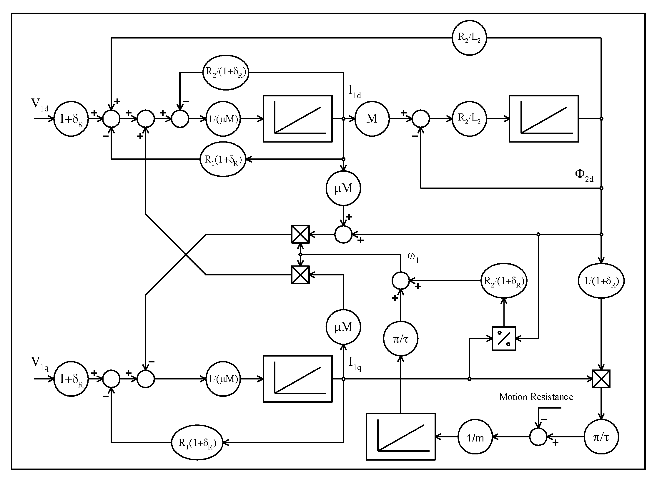
4.1. LIM Performance Control; Adaptive Control

The flux vector-oriented control is one of the most advanced and widely accepted methods used for the rotary machine torque control. It was first conceptualized by Blaschke [76] in 1972 and has been a subject of interest of many researchers ever since, e.g., [77,78,79,80,81,82,83,84,85]. With progress in microprocessor techniques and power electronics, the flux vector-oriented control has become a method of choice for most industrial applications, especially in the development of electric traction propulsion systems, historically based mostly on DC motors, in an effort to replace them with the much less expensive and more robust induction machines. Vector control signifies the independent, or decoupled, control of flux and torque of the motor through coordinated change in the supply voltage and frequency [83]. Flux level control is essential to avoid saturation and minimize core losses under various steady-state operating conditions. As the flux variation tends to be slow, especially with the current control, maintaining constant flux may provide precise torque response and, consequently, a desired speed response.

It is possible to distinguish three flux linkages in the induction machine complex form equations. These flux linkages are the stator flux linkage, the main, or air gap, flux linkage, and the rotor flux linkage. The current decoupling network simplifies only for the rotor flux orientation, whereas the voltage-decoupling network simplifies for the stator flux orientation. Only for a constant rotor flux orientation, the mechanical characteristic does not have a peak value and is a straight line. This linear characteristic is ideal for control application. For a given stator flux in the flux-weakening region and under steady-state operation, however, the stator flux is superior in terms of torque per unit stator current.

Direct Torque Control (DTC) is yet another vector control technique. It was introduced by Depenbrock [84,85] and Takahashi [86] and has been developed by others [87,88]. The fundamental premise of DTC is that a specific DC-link voltage and a specific stator flux establish a unique frequency of inverter operation. This is because the time required by the time integral of the DC-link voltage to integrate up to the reference flux level is unique and represents the half-period time of the frequency of operation. Despite its simplicity, DTC can produce a fast torque response and is robust with respect to transient perturbations and motor parameter detuning [14]. It must also be noted that beside the already mentioned advantages, DTC does not use a modulator and does not employ current control loops, inherent to the vector-oriented flux control. However, during steady-state operation, a pulsation of torque, flux, and current may occur, affecting speed estimation and increasing the acoustic noise. This method is not established so well as the flux-oriented control and has not been applied in LIM controls; however, based on the up-to-date progress in its development, it shows exceedingly high application potential, particularly in the area where parameter sensitivity can be an issue.

Industrial applications of LIM motors require a relatively simple control algorithm because the parameters of industrial process LIMs are well known or can be measured in an off-line experiment. This is not so in urban transit applications since the motors are usually required to operate at peak thrust and the main parameters responsible for the precise peak tracking—the rotor resistance, R₂, and the mutual inductance, M—vary in a very wide range. Thus, the controller of a transit traction LIM should be capable of tracking the maximum available thrust, independent of the air-gap length or the reaction rail construction properties and temperature. Several LIM control methods have been reported thus far, most of them based on the concept of vector control [35]; however, none of them attempt to resolve the parameter adaptation issue. To solve this problem a modified flux vector control technique has been applied [29,43].

The thrust calculated in the rotor flux reference frame compares to measurement only if the rotor parameters, R₂ and L₂, are correctly estimated and their values do not change due to physical or environmental conditions. When these conditions are met, the secondary flux aligns with a d-axis and the back Electro-Motoric Force (EMF) naturally aligns with a q-axis. Should the rotor resistance, R₂, change its value from the set point, the secondary flux would become misaligned and so a non-zero, q-axis component would develop; this means that more voltage is demanded from the supply inverter. This increased voltage generates a negative EMF d-component by advancing the rotor flux. Although the magnitude of the primary current vector remains constant and the secondary flux has increased, the angle between the two vectors has changed and is no longer optimal. A change of the machine secondary resistance from the reference value detunes the controls and a non-zero d-component of the EMF is generated. The optimal operation can be achieved again with the adapted rotor resistance reference value but at a different synchronous frequency. For the magnetizing inductance change, regardless of the cause, e.g., change in air gap, change in the reaction rail geometry, or change in the lamination coarseness or magnetization characteristics of the RR, a q-component of the secondary flux is generated. The induced voltage develops a negative d-component, such as in the case of the secondary resistance detuning. If the value of the reference magnetizing inductance is corrected to equal that of the motor, the controls would become tuned in again and a developed thrust would be optimal, although it would be lower. Since the secondary resistance compensation loop that corrects a d-component of the induced voltage is active, the secondary flux will be regulated to align with the d-axis.

To verify the above parameter compensation control concept in the simulation software, a d–q model of the LIM is first derived, see Figure 9. This LIM signal network clearly shows the impact of parameter detuning on the rotor flux and slip frequency estimation.

To correlate the model and control variables of the d–q system with the real-time three-phase values, standard Clarke and Park transformations are applied [17]. Figure 10a,b shows the simulated response of the system to a step change of R₂ and M both with and without the adaptive compensation control loops.

The adaptive algorithm improves the performance of the system by a significant margin by improving the mechanical output. The proposed algorithm successfully addresses the problem of LIM parameter detuning while preserving all the positive features of the rotor flux referenced vector control. The verification of the simulation results was performed by comparing the calculated output with measurements from a transit test vehicle fitted with the subject test LIM. This method exhibits the robustness necessary in severe transient conditions associated with the application of the LIM in transportation systems.

4.2. LIM Driven from the Voltage Inverter

In all typical LIM simulation models, the symmetrical three-phase current is fed into the three-phase winding to simulate a constant current mode; however, this does not reflect reality when the LIM is driven from the voltage inverter. The differences in slip versus thrust characteristics between the simplified approach and the approach where an asymmetry of phase currents arises naturally from the real supply conditions are presented in [70].

Typically, the LIM is powered from a PWM voltage inverter, converting thrust command into current at a desired frequency. However, as the phase impedances are unequal and the three-phase currents differ in their phase and magnitude, the negative sequence currents are produced leading to a decreased motor performance. In theory, if the LIM phase impedances were known, the phase currents could be equalized, although not entirely, by a proper phase voltage control, but at a price of increased voltage harmonics. The electromagnetic fields shown below (Figure 11) are calculated considering the natural asymmetry of phase currents under symmetrical voltage excitation.

As can be seen from Figure 11, the magnetic field shows significant asymmetry on both ends of the machine. This results in asymmetric coupling and an asymmetric back electromotive force that leads to unequally coupled impedances and the asymmetry of phase currents. Because the phase currents are magnetically coupled with one another and additionally coupled with the induced currents of the reaction rail, these impedances are frequency and speed dependent; thus, their determination can be very involving.

The exemplary performance characteristics of the subject LIM in current and voltage modes for different speeds are shown in Figure 12.

The characteristic increase of peak-thrust slip frequency that can be seen in the figure above results from the end-effect induced magnetizing impedance change. As can be seen from above figure, it is important to account for the asymmetry of phase currents when determining the LIM performance. To do so, the electromagnetic transient FEA simulation with the symmetrical three-phase voltage source would have to be used. However, that would become prohibitively time consuming due to a need of remeshing a large solution space at every time step. Alternatively, the quasi-steady-state transient solution can be achieved by simulating in the frequency domain but only if the software allows for the modification of Ampere’s law.

4.3. Losses in the Reaction Rail

In order to determine the transverse effects of the current flowing in the reaction rail, another numerical FE model should be applied. This can be done using the electric vector potential T, defined by the formula $rotT=J$, where $J$ denotes the current density vector [74,75]. The differential equation for the electrical vector potential can be written as follows (movement only in x-direction is allowed):

$$\frac{{\partial }^{2}T}{\partial x^2}+\frac{{\partial }^{2}T}{\partial y^2}=\mathsf{\sigma }(\frac{\partial B}{\partial t}+v_x\frac{\partial B}{\partial x})$$

(2)

Solving Equation (2) with different values of σ, $v_x$, and f, it is possible to calculate the current density distribution (and other important parameters of the LIM, such as power losses and forces) for any combination of these parameters. Figure 13 shows an example of the current density distribution in the aluminum rail of the LIM for different slip values of constant frequency.

The electric vector potential method can also be applied for the calculation of eddy current distribution in the copper sheet of the rotor due to skewed armature slots (Figure 14a) and for the analysis of influence of the rotor slits on the eddy current distribution in the rotor of rotating induction machines (Figure 14b).

The method presented here has a broader meaning. It is a practical tool that enables the analysis of the power losses in the LIM reaction rail and their minimization. Similar results have also been presented in [55].

4.4. Real-Time Temperature Rise Prediction of a Traction LIM

The enclosed structure of the LIM primary, its continuous movement over the reaction rail, and a large gap between the primary and the reaction rail effectively isolate the primary from the heat flux generated in the RR. For all electric and electronic components and devices for which the heat losses can be determined solely from the electric current measurement, such as cables, inductors, relay coils, linear motors, actuators, etc., the maximum nominal temperature rise above ambient can be directly associated with the value of nominal current. However, the device’s heat-producing current often varies, due to load changes, ranging from zero to values exceeding the value of the nominal current by a large factor. Such complex load cycles can produce highly variable thermal cycling and result in uncontrolled over-temperature, which negatively impacts the life cycle of a device. During the acceleration and deceleration of a LIM-powered electric traction vehicle, the instantaneous current of the motor exceeds, by a high margin, the nominal thermal value and then decreases below that value during coasting and drops to zero at station stops, therefore undergoing severe thermal cycling. The basic heat equation describes the balance between the dissipated, stored, and radiated heat. The dissipated heat will be partially transferred into the surrounding ambient and partially stored in the heated device by increasing its temperature. So long as the heat power is constant, the temperature rise will achieve a maximum value of $\Delta T_{max}$, and the thermal transient state will be described by the following equation [91]:

$$\Delta T=\Delta T_{max}\left(1-e^{-\frac{t}{\tau }}\right)+\Delta T_0{e}^{-\frac{t}{\tau }}$$

(3)

where ΔT₀ is the temperature rise over ambient at t = 0, $\Delta T_{max}$ is the maximum temperature rise over ambient for $t\to \infty$, and $\tau$ is a characteristic constant (thermal time constant).

Equation (3) is frequently used to determine an initial temperature rise estimation of a device undergoing thermal cycling by solving it for the thermal cycle average rms current. However, this approach leads to an error in temperature prediction as it does not account for the temperature dependence of a heat power source. This problem was solved in [91] by correcting and then solving the conventional differential equation/algorithm and providing an exact solution that utilized a single heat-run-test data point. The temperature prediction performance of the basic and improved equations was analyzed by calculating the temperature rise of a linear motor subjected to a typical, nominal service duty cycle. The simulation took into consideration the result of a thermal test performed during a thermal qualification of the subject LIM. The simulation results were further compared against the results of temperature measurement taken from a thermal sensor imbedded in a production LIM’s winding while operating the LIM-powered vehicle with the nominal load on the existing Vancouver Expo line system. The experimental data in the form of motor temperature and phase current were collected and overlayed with the simulation results. The results (see Figure 15) confirm that the improved algorithm (blue) predicts the LIM temperature rise (green) with much better accuracy than the basic algorithm (red). The measured temperature is still lower than the improved prediction, mainly due to an additional cooling effect resulting from the increased convection of a moving train. Because of a high degree of prediction accuracy and minimal application cost, the improved software algorithm found practical application and had been installed fleet wide.

The efficiency of a traction LIM motor, as has already been mentioned, is rather low and in the case of a loss of forced cooling high losses can drive the temperature of the center of the winding quickly to above the maximum allowed level. Precise detection of this process is important as it allows the train control system to maintain the LIM in operation for as long as possible without compromising the insulation life cycle. Figure 16 shows the typical dependencies of power factor and efficiency for a traction LIM applied on most urban transportation systems in the world. These results were confirmed by experimental measurements taken by one of the authors for the motor, which now operates on a Rapid KL Rail System in Kuala Lumpur, Malaysia. It characterizes similarly built traction LIMs of comparable size and cooling efficiency.

4.5. Superconductig LIM

A typical linear induction motor with an iron core and copper windings can only produce limited thrust because of the saturation of the iron core and, in particular, its teeth. Superconducting Linear Induction Motors (SLIMs) are a promising alternative to conventional traction solutions. A novel high-temperature superconducting (HTSC) SLIM was proposed in [26]. This SLIM uses stacks of second generation (2G) superconducting tapes. Such a SLIM, capable of high ampere turns, can generate a strong magnetic field and, consequently, exceptionally large thrust as it can achieve high flux densities over wide air gaps. Commercial 2G HTS tapes utilizing yttrium- and gadolinium-based ceramics (YBCO) can operate up to critical temperatures of 77 K, which can be provided by liquid nitrogen refrigerants. They can carry a critical current of 600 A at 77 K and self-field. These properties make 2G tapes a promising material for use in power electric equipment, including rotating and linear induction machines [23,24,25].

The conventional variant of such a SLIM has already been analyzed in [29,61,70]. The only additional component of the SLIM is the cryostat, as in [24].

To determine all the crucial parameters of the SLIM, the FEA has been applied. One of the challenges that must be solved is a proper evaluation of penetration of the strong electromagnetic field into the moving and conducting reaction rail. Such modeling and analysis can be extremely difficult and time consuming as it requires a proper choice of the FE mesh (depending on the velocity and slip) [70]. Because of the strong saturation of the laminated magnetic core, classical LIM construction methods may be put into question.

The current density within the HTSC coil was modeled according to the power law for superconducting windings [14]. Figure 17a shows an example of the magnetic field distribution within the subject SLIM, and Figure 17b shows the thrust characteristics for different speeds.

As can be seen from the figures above, the superconducting LIM has significantly increased thrust values compared to a conventional solution. An important computational problem here is the correct modeling of the superconducting windings in the LIM, as well as the correct consideration of the strong saturation of the magnetic circuit.

5. Conclusions

The paper provides an overview of different linear transportation systems and focuses on the applications that use linear induction motors. Against this background, the authors have presented and discussed new practical methodologies capable of solving some important transportation LIM problems. Despite the LIM’s lower efficiency, when compared with the rotary motor, for many applications the LIM system is a superior transport solution that successfully competes against the conventional, rotary-motor-based alternative. This is because the efficiency is a broader concept and the efficiency of a transportation system must be analyzed in the context of the application. For elevated, driverless automated systems, the LIM is indeed a superior solution because it does not rely on adhesion, has no moving parts, and provides the lowest life cycle and operation and maintenance costs.

Based upon the experience gathered in the subject area of LIMs, the authors believe that future research work should concentrate on increasing the motor efficiency by improving the construction materials and production technology and researching the application of high-temperature superconductivity. This progress must be accompanied by the improvement in efficiency of predictive algorithms and more efficient FEA methods.

LIMs have been known and widely researched by the scientific community but mostly as standalone electric motors. However, LIMs often work as parts of an overly complex transportation system. Thus, future research should take into account the complex interaction of the LIM with its specific system environment.

References

1. Hellinger, R.; Mnich, P. Linear motor-powered transportation: History, present status, and future outlook. Proc. IEEE 2009, 97, 1892–1900. [Google Scholar] [CrossRef]
2. Woronowicz, K.; Safaee, A. A novel linear induction motor equivalent-circuit with optimized end effect model. Can. J. Electr. Comput. Eng. 2014, 37, 34–41. [Google Scholar] [CrossRef]
3. Woronowicz, K. Urban Mass Transit Systems: Current Status and Future Trends. In Proceedings of the ITEC 2014, Cologne, Germany, 13 August 2014. [Google Scholar]
4. Byers, D.C. The Linear Induction Motor in Transit, a System View. In Proceedings of the 5th International Conference on Automated People Movers, Paris, France, 10–14 June 1996. [Google Scholar]
5. Earnshaw, S. On the Nature of the Molecular Forces which regulate the Constitution of the Luminiferous Ether. Trans. Camb. Philos. Soc. 1842, 7, 97–112. [Google Scholar]
6. Weh, H.; Steingröver, A.; Hupe, H. Design and Simulation of a Controlled Permanent Magnet. Int. J. Appl. Electromagn. Mater. 1992, 3, 199–203. [Google Scholar]
7. Palka, R. Synthesis of magnetic fields by optimization of the shape of areas and source distributions. Electr. Eng. 1991, 75, 1–7. [Google Scholar] [CrossRef]
8. Sikora, R.; Palka, R. Synthesis of Magnetic-Fields. IEEE Trans. Magn. 1982, 18, 385–390. [Google Scholar] [CrossRef]
9. Braunbeck, W. Freely Suspended Bodies in Electric and Magnetic Fields. Z. Phys. 1938, 112, 753–763. [Google Scholar]
10. May, H.; Palka, R.; Portabella, E.; Canders, W.-R. Evaluation of the magnetic field – high temperature superconductor interactions. Int. J. Comput. Math. Electr. Electron. Eng. 2004, 23, 286–304. [Google Scholar] [CrossRef]
11. Patel, A.; Hopkins, S.; Giunchi, G.; Figini Albisetti, A.; Shi, Y.; Palka, R.; Cardwell, D.; Glowacki, B. The Use of an MgB2 Hollow Cylinder and Pulse Magnetized (RE)BCO Bulk for Magnetic Levitation Applications. IEEE Trans. Appl. Supercond. 2013, 23, 6800604. [Google Scholar] [CrossRef]
12. Masada, E. Development of Maglev and Linear Drive Technology for Transportation in Japan. In Proceedings of the MAGLEV’95, Bremen, Germany, 26–29 November 1995; ISBN 3-8007-2155-4. [Google Scholar]
13. Ji, W.; Jeong, G.; Park, C.; Jo, I.; Lee, H. A Study of Non-Symmetric Double-Sided Linear Induction Motor for Hyperloop All-In-One System (Propulsion, Levitation, and Guidance). IEEE Trans. Magn. 2018, 54, 1–4. [Google Scholar] [CrossRef]
14. Ma, G.; Wang, Z.; Liu, K.; Qian, H.; Wang, C. Potentials of an Integrated Levitation, Guidance, and Propulsion System by a Superconducting Transverse Flux Linear Motor. IEEE Trans. Ind. Electron. 2018, 65, 7548–7557. [Google Scholar] [CrossRef]
15. Lee, C.Y.; Jo, J.M.; Han, Y.J.; Bae, D.K.; Yoon, Y.S.; Choi, S.; Park, D.K.; Ko, T.K. Estimation of Current Decay Performance of HTS Electromagnet for Maglev. IEEE Trans. Appl. Supercond. 2010, 20, 907–910. [Google Scholar]
16. Woronowicz, K. Linear motor drives and applications in rapid transit systems. In Proceedings of the Transportation Electrification Conference and Expo (ITEC), Detroit, MI, USA, 15–18 June 2014. [Google Scholar]
17. Nasar, S.A.; Boldea, I. Linear Motion Electric Machines; John Wiley & Sons: New York, NY, USA, 1976. [Google Scholar]
18. Cao, R.; Lu, M.; Jiang, N.; Cheng, M. Comparison between Linear Induction Motor and Linear Flux-Switching Permanent-Magnet Motor for Railway Transportation. IEEE Trans. Ind. Electron. 2019, 66, 9394–9405. [Google Scholar] [CrossRef]
19. Weh, H. Linear Electromagnetic Drives in Traffic Systems and Industry. In Proceedings of the LDIA’95, Nagasaki, Japan, 31 May–2 June 1995. [Google Scholar]
20. Cao, R.; Lu, M. Investigation of High Temperature Superconducting Linear Flux-Switching Motors With Different Secondary Structures. IEEE Trans. Appl. Supercond. 2020, 30, 1–5. [Google Scholar] [CrossRef]
21. Ma, G.; Gong, T.; Zhang, H.; Wang, Z.; Li, X.; Yang, C.; Liu, K.; Zhang, W. Experiment and Simulation of REBCO Conductor Coils for an HTS Linear Synchronous Motor. IEEE Trans. Appl. Supercond. 2017, 27, 1–5. [Google Scholar] [CrossRef]
22. Liu, B.; Badcock, R.; Shu, H.; Fang, J. A Superconducting Induction Motor with a High Temperature Superconducting Armature: Electromagnetic Theory, Design and Analysis. Energies 2018, 11, 792. [Google Scholar] [CrossRef] [Green Version]
23. Liu, J.; Ma, H.; Cheng, J. Research on Superconducting Induction Maglev Linear Machine for Electromagnetic Launch Application. IEEE Trans. Plasma Sci. 2017, 45, 1644–1650. [Google Scholar] [CrossRef]
24. Sotelo, G.G.; Sass, F.; Carrera, M.; Lopez-Lopez, J.; Granados, X. Proposal of a Novel Design for Linear Superconducting Motor Using 2G Tape Stacks. IEEE Trans. Ind. Electron. 2018, 65, 7477–7484. [Google Scholar] [CrossRef] [Green Version]
25. Chen, X.; Zheng, S.; Li, J.; Ma, G.T.; Yen, F. A linear induction motor with a coated conductor superconducting secondary. Phys. C Supercond. Appl. 2018, 550, 82–84. [Google Scholar] [CrossRef]
26. Palka, R.; Woronowicz, K.; Kotwas, J. Analysis of the Performance of Superconducting Linear Induction Motors. In Proceedings of the CEFC 2020, Pisa, Italy, 16–19 November 2020. [Google Scholar]
27. Kircher, R.; Klühspies, J.; Palka, R.; Fritz, E.; Eiler, K.; Witt, M. Electromagnetic Fields Related to High Speed Transportation Systems. Transp. Syst. Technol. 2018, 4, 152–166. [Google Scholar] [CrossRef] [Green Version]
28. Woronowicz, K.; Safaee, A. A novel linear induction motor equivalent-circuit with optimized end-effect model including partially-filled end slots. In Proceedings of the Transportation Electrification Conference and Expo (ITEC), Detroit, MI, USA, 15–18 June 2014. [Google Scholar]
29. Woronowicz, K.; Palka, R. Optimised Thrust Control of Linear Induction Motors by a Compensation Approach. Int. J. Appl. Electromagn. Mech. 2004, 19, 533–536. [Google Scholar] [CrossRef]
30. Woronowicz, K.; Palka, R. An advanced linear induction motor control approach using the compensation of its parameters. In Electromagnetic Fields in Electrical Engineering; IOS Press: Amsterdam, The Netherlands, 2002; pp. 335–338. [Google Scholar]
31. Gieras, J.; Dawson, G.; Eastham, A. Performance calculation for single-sided linear induction motors with a double-layer reaction rail under constant current excitation. IEEE Trans. Magn. 1986, 22, 54–62. [Google Scholar] [CrossRef]
32. Mendrela, E.A.; Gierczak, E. Two-dimensional analysis of linear induction motor using Fourier’s series method. Electr. Eng. 1982, 65, 97–106. [Google Scholar] [CrossRef]
33. Nasar, S.A.; del Cid, L. Certain approaches to the analysis of single-sided linear induction motors. Proc. Inst. Electr. Eng. 1973, 120, 477–483. [Google Scholar] [CrossRef]
34. Freeman, E.M.; Lowther, D.A. Normal force in single-sided linear induction motors. Proc. Inst. Electr. Eng. 1973, 120, 1499–1506. [Google Scholar] [CrossRef]
35. Yamamura, S. Theory of Linear Induction Motors, 2nd ed.; Halster Press: New York, NY, USA, 1979. [Google Scholar]
36. Borcherts, R.H.; Reitz, J.R. High-speed transportation via magnetically supported vehicles: A study of the magnetic forces. Transp. Res. 1971, 5, 197–209. [Google Scholar] [CrossRef]
37. Fink, H.J. Instability of vehicles levitated by eddy current repulsion-case of an infinitely long current loop. J. Appl. Phys. 1971, 42, 3446. [Google Scholar] [CrossRef]
38. Reitz, J.R. Force on a rectangular coil moving above a conducting slab. J. Appl. Phys. 1972, 43, 1547. [Google Scholar] [CrossRef]
39. Langerholc, J. Torques and forces on a moving coil due to eddy currents. J. Appl. Phys. 1973, 44, 1587. [Google Scholar] [CrossRef]
40. Lee, S.-W.; Menendez, R. Force on current coils moving over a conducting sheet with application to magnetic levitation. Proc. IEEE 1974, 62, 567–577. [Google Scholar]
41. Tegopoulos, J.A.; Kriezis, E.E. Eddy Currents in Linear Conducting Media; Elsevier Science: New York, NY, USA, 1985. [Google Scholar]
42. Adamiak, K. A method of optimization of winding in linear induction motor. Electr. Eng. 1986, 69, 83–91. [Google Scholar] [CrossRef]
43. Kim, D.-K.; Kwon, B.-I. A novel equivalent circuit model of the linear induction motor based on finite element analysis and its coupling with external circuits. IEEE Trans. Magn. 2006, 42, 3407–3409. [Google Scholar] [CrossRef]
44. Gieras, J.F.; Dawson, G.E.; Easthan, A.R. A new longitudinal end effect factor for linear induction motor. IEEE Trans. Energy Convers. 1987, 2, 152–159. [Google Scholar] [CrossRef]
45. Satvati, M.R.; Vaez-Zadeh, S. End-effect compensation in linear induction motor drives. J. Power Electron. 2011, 11, 697–703. [Google Scholar] [CrossRef] [Green Version]
46. Duncan, J. Linear induction motor—Equivalent-circuit model. IEEE Proc. B Electr. Power Appl. 1983, 130, 51–57. [Google Scholar] [CrossRef]
47. Xu, W.; Zhu, J.G.; Zhang, Y.; Li, Y.; Wang, Y.; Guo, Y. An Improved Equivalent Circuit Model of a Single-Sided Linear Induction Motor. IEEE Trans. Veh. Technol. 2010, 59, 2277–2289. [Google Scholar] [CrossRef] [Green Version]
48. Xu, W.; Zhu, J.G.; Zhang, Y.; Li, Z.; Li, Y.; Wang, Y.; Guo, Y.; Li, Y. Equivalent Circuits for Single-Sided Linear Induction Motors. IEEE Trans. Ind. Appl. 2010, 46, 2410–2423. [Google Scholar] [CrossRef] [Green Version]
49. Lv, G.; Zeng, D.; Zhou, T. An Advanced Equivalent Circuit Model for Linear Induction Motors. IEEE Trans. Ind. Electron. 2018, 65, 7495–7503. [Google Scholar] [CrossRef]
50. Zeng, D.; Lv, G.; Zhou, T. Equivalent circuits for single-sided linear induction motors with asymmetric cap secondary for linear transit. IEEE Trans. Energy Convers. 2018, 33, 1729–1738. [Google Scholar] [CrossRef]
51. Dmitrievskii, V.; Goman, V.; Sarapulov, F.; Prakht, V.; Sarapulov, S. Choice of a numerical differentiation formula in detailed equivalent circuits models of linear induction motors. In Proceedings of the 2016 International Symposium on Power Electronics, Electrical Drives, Automation and Motion (SPEEDAM), Capri, Italy, 22–24 June 2016; pp. 458–463. [Google Scholar]
52. Zare-Bazghaleh, A.; Naghashan, M.; Khodadoost, A. Derivation of Equivalent Circuit Parameters for Single-Sided Linear Induction Motors. IEEE Trans. Plasma Sci. 2015, 43, 3637–3644. [Google Scholar] [CrossRef]
53. Sung, J.-H.; Nam, K. A new approach to vector control for a linear induction motor considering end effects. In Proceedings of the IEEE Industry Applications Society, Thirty-Fourth IAS Annual Meeting, Phoenix, AZ, USA, 3–7 October 1999; Volume 4, pp. 2284–2289. [Google Scholar]
54. Huang, C.-I.; Hsu, K.-C.; Chiang, H.-H.; Kou, K.-Y.; Lee, T.-T. Adaptive fuzzy sliding mode control of linear induction motors with unknown end effect consideration. In Proceedings of the International Conference on Advanced Mechatronic Systems, Tokyo, Japan, 18–21 September 2012; pp. 626–631. [Google Scholar]
55. Shiri, A.; Shoulaie, A. Design optimization and analysis of single-sided linear induction motor, considering all phenomena. IEEE Trans. Energy Convers. 2012, 27, 516–525. [Google Scholar] [CrossRef]
56. Pucci, M. Direct field oriented control of linear induction motors. Electr. Power Syst. Res. 2012, 89, 11–22. [Google Scholar] [CrossRef]
57. Shiri, A.; Shoulaie, A. End effect braking force reduction in high-speed single-sided linear induction machine. Energy Convers. Manag. 2012, 61, 43–50. [Google Scholar] [CrossRef]
58. Kang, G.; Nam, K. Field-oriented control scheme for linear induction motor with the end effect. IET Electr. Power Appl. 2005, 152, 1565–1572. [Google Scholar] [CrossRef]
59. Accetta, A.; Cirrincione, M.; Pucci, M.; Vitale, G. MRAS speed observer for high performance linear induction motor drives based on linear neural networks. In Proceedings of the IEEE Energy Conversion Congress and Exposition, Phoenix, AZ, USA, 17–22 September 2011; pp. 1765–1772. [Google Scholar]
60. Mirsalim, M.; Doroudi, A.; Moghani, J.S. Obtaining the operating characteristics of linear induction motors: A new approach. IEEE Trans. Magn. 2002, 38, 1365–1370. [Google Scholar] [CrossRef]
61. Abdelqader, M.; Morelli, J.; Palka, R.; Woronowicz, K. 2-D quasi-static solution of a coil in relative motion to a conducting plate. Int. J. Comput. Math. Electr. Electron. Eng. 2017, 36, 980–990. [Google Scholar] [CrossRef]
62. Woronowicz, K.; Abdelqader, M.; Palka, R.; Morelli, J. 2-D quasi-static Fourier series solution for a linear induction motor. Int. J. Comput. Math. Electr. Electron. Eng. 2018, 37, 1099–1109. [Google Scholar] [CrossRef]
63. Freeman, E.M.; Papageorgiou, C.D. Spatial Fourier transforms: A new view of end effects in linear induction motors. Proc. Inst. Electr. Eng. 1978, 125, 747–7753. [Google Scholar] [CrossRef]
64. Paudel, N.; Bird, J.Z. General 2-D steady-state force and power equations for a traveling time-varying magnetic source above a conductive plate. IEEE Trans. Magn. 2012, 48, 95–100. [Google Scholar] [CrossRef]
65. Lee, S.; Lee, H.; Ham, S.; Jin, C.; Park, H.; Lee, J. Influence of the construction of secondary reaction plate on the transverse edge effect in linear induction motor. IEEE Trans. Magn. 2009, 45, 2815–2818. [Google Scholar]
66. Singh, M.; Khajuria, S.; Marwaha, S. Thrust analysis and improvement of single sided linear induction motor using finite element technique. Int. J. Curr. Eng. Technol. 2013, 3, 563–566. [Google Scholar]
67. Jeong, J.; Lim, J.; Park, D.; Choi, J.; Jang, S. Characteristic analysis of a linear induction motor for 200-km/h maglev. Int. J. Railw. 2015, 8, 15–20. [Google Scholar] [CrossRef] [Green Version]
68. Abdollahi, S.E.; Mirzayee, M.; Mirsalim, M. Design and analysis of a double-sided linear induction motor for transportation. IEEE Trans. Magn. 2015, 51, 1–7. [Google Scholar] [CrossRef]
69. Amiri, E.; Mendrela, E.A. A novel equivalent circuit model of linear induction motors considering static and dynamic end effects. IEEE Trans. Magn. 2014, 50, 120–128. [Google Scholar] [CrossRef]
70. Palka, R.; Woronowicz, K.; Kotwas, J.; Xing, W.; Chen, H. Influence of different supply modes on the performance of linear induction motors. Arch. Electr. Eng. 2019, 68, 473–483. [Google Scholar]
71. De Gersem, H.; Vande Sande, H.; Hameyer, K. Motional magnetic finite element method applied to high speed rotating devices. Int. J. Comput. Math. Electr. Electron. Eng. 2000, 19, 446–451. [Google Scholar]
72. De Gersem, H.; Hameyer, K. Finite element simulation of a magnetic brake with a soft magnetic solid iron rotor. Int. J. Comput. Math. Electr. Electron. Eng. 2002, 21, 296–306. [Google Scholar] [CrossRef] [Green Version]
73. Introduction to COMSOL Multiphysics, Version 5.6, ©1998–2020 COMSOL. Available online: https://www.comsol.com/documentation (accessed on 25 February 2021).
74. Sikora, R.; Lipinski, W.; Gawrylczyk, K.; Gramz, M.; Palka, R.; Ziolkowski, M. Analysis of the magnetic field in the end region of induction motor. IEEE Trans. Magn. 1982, 18, 674–678. [Google Scholar] [CrossRef]
75. Sikora, R.; Gawrylczyk, K.; Gramz, M.; Gratkowski, S.; Ziolkowski, M. Magnetic field Computation in the End-Region of Electric Machines Using Various Boundary Conditions on Iron Surfaces. IEEE Trans. Magn. 1986, 22, 204–207. [Google Scholar] [CrossRef]
76. Blaschke, F. The Principle of Field Orientation as Applied to the New Transvector Closed-Loop Control System for Rotating Machines. Siemens Rev. 1972, 34, 217–220. [Google Scholar]
77. Trzynadlowski, A. The Field Orientation Principle in Control of Induction Motors; Kluwer Academic Publishers: Amsterdam, The Netherlands, 1994. [Google Scholar]
78. Boldea, I.; Nasar, S.A. Vector Control of AC Drives; CRC Press: London, UK, 1992. [Google Scholar]
79. Leonhard, W. Control of Electric Drives; Springer: Berlin, Germany, 1985. [Google Scholar]
80. Kaźmierkowski, M.P.; Tunia, H. Automatic Control of Converter-Fed Drives; Elsevier: Amsterdam, The Netherlands, 1994. [Google Scholar]
81. Kovács, P.K. Transient Phenomena in Electric Machines; Elsevier: Amsterdam, The Netherlands, 1984. [Google Scholar]
82. Yamamura, S. AC Motors for High Performance Applications: Analysis and Control; Marcel Dekker: New York, NY, USA, 1986. [Google Scholar]
83. Lipo, T.; Novotny, D. Principles of Vector Control and Field Estimation. In Introduction to Field Orientation and High Performance Drives; IEEE Tutorial Course: Minneapolis, MN, USA, 1985. [Google Scholar]
84. Depenbrock, M. Direkte Selbstregelung (DSR) für hochdynamische Drehfeldantriebe mit Stromrichterspeisung. etz-Archiv 1985, 7, 211–218. [Google Scholar]
85. Depenbrock, M. Direct Self-Control of the Flux and Rotary Moment of a Rotary-Field Machine. U.S. Patent 4,678,248, 7 July 1987. [Google Scholar]
86. Takahashi, I.; Noguchi, T. A new quick response and high efficiency control strategy of an induction motor. IEEE Trans. Ind. Appl. 1986, IA-22, 820–827. [Google Scholar] [CrossRef]
87. Tiitinen, P.; Pohjalainen, P.; Lalu, J. The next generation motor control method–Direct torque control (DTC). Eur. Power Electron. Drives 1995, 5, 14–18. [Google Scholar]
88. Kazmierkowski, M.; Kasprowicz, A. Improved direct torque and flux vector control of PWM inverter-fed induction motor drives. IEEE Trans. Ind. Electron. 1995, 42, 344–350. [Google Scholar] [CrossRef]
89. May, H.; Canders, W.-R.; Palka, R. Loss reduction in synchronous machines by appropriate feeding patterns. In Proceedings of the International Conference on Electrical Machines ICEM ’98, Istanbul, Turkey, 2–4 September 1998. [Google Scholar]
90. May, H.; Palka, R.; Canders, W.-R. Optimized control of induction machines for dynamic torque requirements. In Electromagnetic Fields in Electrical Engineering; IOS Press: Amsterdam, The Netherlands, 2002; pp. 254–259. [Google Scholar]
91. Woronowicz, K.; Safaee, A.; Maknouninejad, A. Enhanced Algorithm for Real Time Temperature Rise Prediction of a Traction LIM. In Proceedings of the Transportation Electrification Conference and Expo, ITEC 2018, Long Beach, CA, USA, 13–15 June 2018; pp. 616–620. [Google Scholar]
Figure 1. Conversion of rotary machine into LIM.
Energies 14 02549 g001
Figure 2. Short-primary LIM (a); short-secondary LIM (b).
Energies 14 02549 g002
Figure 3. LIM primary (supplied part) (a); LIM secondary (reaction rail) (b) [28].
Energies 14 02549 g003
Figure 4. Three-dimensional model of the LIM [29].
Energies 14 02549 g004
Figure 5. Two filaments 2x0 apart, placed at a distance g above the conducting plate of thickness d [61] (a). The back iron and primary iron are additionally modeled as two infinite layers with zero conductivity and infinite permeability (b).
Energies 14 02549 g005
Figure 6. Average horizontal force density (a) and average vertical force density (b) acting on the coil as a function of frequency for different LIM velocities [61].
Energies 14 02549 g006
Figure 7. Evolution of 2D models of the LIM used for the numerical field evaluation. Idealized coils of a three-phase, six-pole machine [62] (a). Full model of the LIM [70] (b).
Energies 14 02549 g007
Figure 8. Average thrust per unit depth versus slip frequency for a LIM from Figure 7 [62].
Energies 14 02549 g008
Figure 9. Rotor flux-oriented control LIM model [29,30].
Energies 14 02549 g009
Figure 10. Response to a step of the secondary resistance R2 (a); response to a step of the mutual inductance M (b) [29].
Energies 14 02549 g010
Figure 11. Magnetic field distribution within the LIM [70].
Energies 14 02549 g011
Figure 12. LIM characteristics obtained for the current supply (I = 550 A) (a) and the voltage supply (V = 460 V) (b) [70].
Energies 14 02549 g012
Figure 13. Current density distribution in the rail of the LIM with constant frequency and different slip values [29].
Energies 14 02549 g013
Figure 14. Eddy current distribution in the copper sheet of the rotor due to skewed armature slots (a). Influence of the rotor slits on eddy current distribution in the rotor (b) [89,90].
Energies 14 02549 g014
Figure 15. Comparison of different algorithms of temperature rise versus measured temperature results [91].
Energies 14 02549 g015
Figure 16. Power factor and efficiency curves for one example of a traction LIM.
Energies 14 02549 g016
Figure 17. Magnetic field distribution within the end part of the SLIM (a). SLIM characteristics for different speeds (b) [26].
Energies 14 02549 g017
Publisher’s Note: MDPI stays neutral with regard to jurisdictional claims in published maps and institutional affiliations.